Optimization of Magnetization Roasting and Magnetic Separation for the Recovery of Iron from Low-Grade Iron Plant Tailings

Abstract

This study employs response surface methodology (RSM) with a custom optimal design to develop and optimize iron (Fe) grade and recovery through magnetization roasting followed by induced dry-roll magnetic separation. The relationships between the independent and dependent variables are investigated. The effect of roasting temperature, magnetization roasting time, magnetic field intensity, rotor speed, and product splitter position for the induced dry-roll magnetic separator on Fe grade and recovery are studied. Suitable models are generated to predict the optimum operating conditions. An analysis of Variance (ANOVA) is employed to validate the developed regression models’ adequacy and assess the main and interaction-related effects on Fe grade and recovery. During magnetization roasting, a satisfactory Fe grade of 66.8% with a recovery of 16.7% was obtained under optimal conditions of 1050 °C for 97 min. Conversely, after the induced dry-roll magnetic separator optimization, an Fe grade of 66.1% with a recovery of 60.2% was achieved under optimum conditions of 0.105 T for magnetic field intensity, 70 Hz for rotor speed, and an 11 mm product splitter position. This study effectively illustrates how RSM can model the processes of magnetization roasting and induced dry-roll magnetic separation, particularly concerning the operating parameters used for treating iron ore plant tailings. Furthermore, it highlights the efficiency of this methodology in generating substantial insights in a short timeframe while minimizing the number of experiments conducted.

1. Introduction

Iron is a vital metal that is crucial in advancing modern societies [1]. It constitutes approximately 95% of all metals utilized annually across various sectors, including in structural engineering, maritime, automotive, and general industrial applications [2]. The continuous rise in steel demand has led to a marked increase in the extraction of crude iron, resulting in the gradual depletion of high-grade iron ore reserves [3]. Consequently, there is a pressing need to process iron from secondary sources such as low-grade iron ores, fines/slimes, and tailings to satisfy the growing requirement for high-quality iron in steel production. The extraction of iron ore generates substantial amounts of tailings and fines, which accumulate in tailing dams and pose various environmental challenges [3]. The average iron content in these tailings is estimated to be around 40%, and, over extended periods of production, this can lead to excessive residue accumulation. This issue is particularly significant in operations that target lower-grade iron ores. According to reports by Dauce et al. (2019) [4] and Yang et al. (2018) [5], the annual generation of iron ore tail (IOT) ranges from approximately 632 million tonnes to 1.4 billion tonnes, highlighting its potential as a secondary source of iron to meet ever-increasing market demand.

Despite this potential value, few commercial operations aim to extract iron from tailings for industrial use. This is mainly due to the complex mineralogy of the tailings, which contain a high amount of gangue material and present challenges in liberating the iron minerals [6]. Traditional beneficiation technologies, such as wet magnetic separation, leaching, microwave roasting, sulfidation roasting, sodium carbonate (Na₂CO₃) roasting, flotation, and some gravity concentrations such as shaking table, jig, reflux classifier, teetered bed separator, multi-gravity separator, and spiral demonstrate some limitations in recovering iron from difficult-to-treat iron-bearing secondary sources.

Although several investigations on the recovery of iron from low-grade iron ore were also achieved using flotation through reverse anionic quartz flotation, magnetic separation remains one of the most effective separation methods to beneficiate iron. However, it has been found that most low-grade iron ores typically contain considerable amounts of hematite occurring together with siderite and limonite, which are characterized by a paramagnetic behavior, making them a refractory and challenging to treat using magnetic separation [7]. Recently, a new pyrometallurgical pretreatment method, based on the chemical transformation of paramagnetic Fe into ferromagnetic minerals such as magnetite (Fe₃O₄) or maghemite (γ-Fe₂O₃), suitable for magnetic separation using pyrometallurgical processing (e.g., magnetizing roasting) followed by conventional magnetic separation, has been developed [7,8]. Several studies have demonstrated that the transformation of iron ores under thermal pretreatment can be enhanced during free moisture removal at temperatures ranging from 120 to 140 °C, followed by the dehydroxylation of limonite when the temperature ranges between 250 °C and 350 °C. Further increases in temperature between 490 °C and 630 °C lead to siderite decomposition, while hematite’s conversion into magnetite occurs at around 850 °C [9,10].

Magnetization roasting has emerged as an attractive area of research and is becoming a promising technology for producing high-quality iron concentrates from low-grade ores and secondary iron sources [6,9,11,12,13,14,15,16,17,18]. The process consists of a partial reductive roasting process that transforms hematite iron oxide with a high oxidative state (Fe³⁺) into magnetite, a ferrimagnetic compound with a lower oxidative state (Fe²⁺). This reduction occurs under oxygenated conditions in the presence of carbon, which, at high temperatures, leads to CO₂ generation due to the oxygen (O₂) contained in the air being responsible for the boudoir reaction occurrence and producing the CO promoting an exothermic reaction where the ratio CO/CO₂ must be carefully regulated to monitor the reduction of hematite into magnetite [19]. After magnetization roasting, the resulting product is subjected to low-intensity magnetic separation to effectively remove impurities such as alumina (Al₂O₃) and silica (SiO₂) from the roasted sample [20].

Different reductants are used during the reduction process; the reductants, amongst others, include coking coal and agro-industrial-biomass, such as straw type (corn straw, rice), sawdust, starch, cow dung, etc. The choice of using biomass as opposed to conventional coking coal is because of its advantageous characteristics, which means it falls under the renewable category and provides a green process [18]. The use of biomass addresses the current SO₂, NO_x, and CO₂ emission challenges by using coal as a reducing agent [21,22]. Additionally, biomass naturally has a high amount of volatile carbonaceous matter, which creates additional reducing gases such as methane (CH₄), hydrogen (H₂), carbon dioxide (CO₂), and carbon monoxide (CO). Therefore, CO is not the only reducing agent, as in the case of coal, which helps in generating more heat and accelerates the reduction process [15].

The current study aims to determine the impact of various parameters on the recovery and grade of iron (Fe) during magnetization roasting, followed by an induced dry-roll magnetic separator. A design of experiment (DoE) methodology using response surface methodology (RSM) and an optimal custom design was employed to optimize the beneficiation process. Therefore, this was achieved by utilizing a systematic approach incorporating multidimensional combinations of input variables in an optimal response surface methodology design. This approach helps to identify the optimal working conditions for achieving satisfactory iron grade and recovery.

2. Materials and Methods

2.1. Materials

The reductants used in this study were macadamia nutshells, which were crushed and pulverized to a size that could pass through a 100 µm sieve. The specifications for the reducing agents were analyzed using proximate and ultimate analyses. The moisture, volatile matter, and ash content were analyzed using a muffle furnace, model AAF 11/3, manufactured by Carbolite Gero Ltd., Sheffield, United Kingdom. The calorific value was analyzed using a combustion calorimeter, model CAL3K-F, manufactured by DDS CALORIMETERS, Randburg, South Africa. The ultimate analyses were performed using a CHNS analyser, model flash 2000, manufactured by Thermofisher scientific, Sunnyvale, CA, USA. The results are detailed in

Table 1. Analysis of macadamia nutshells.

CV (MJ/kg)	Proximate Analysis (%)				Ultimate Analysis (%)
	Moisture	VM	FC	Ash	Sulfur (S)	Carbon (C)	Hydrogen (H)	Nitrogen (N)
18.565	8.71	74.90	14.20	2.18	0.767	48.29	5.43	0.35

CV—calorific value, VM—volatile matter, FC—fixed carbon.

.

About 100 kg of a representative sample was collected from the iron plant tailings dam located in the Kathu District of South Africa’s Northern Cape province. This sample was then crushed in a closed-circuit crusher to achieve a particle size of 100% passing 2 mm, using a Laboratory Roll Crusher, model WT-1873-2, manufactured by Metso, Denver, CO, USA. After crushing, the sample was homogenized and prepared for subsequent characterization and optimization studies.

Particle size distribution analysis was conducted on a 5000 g sample using a vibratory sieve shaker with manual amplitude adjustment settings ranging from 0.5 to 3 mm, model Analysette 3 SPARTAN, manufactured by Fritsch, Idar-Oberstein, Germany. The sequence of wire mesh sieves used was determined following the U.S. Standard Scale ratio, based on the square root of 2. The chemical composition of the head sample was analyzed using an X-ray fluorescence (XRF) model ZSX Primus II, manufactured by Rigaku, Tokyo, Japan, equipped with EZScan software, version 3. The phase analysis was also performed on the head sample using an X-ray diffractometer (XRD), model Ultima IV, manufactured by Rigaku, Tokyo, Japan, to determine the mineralogical species equipped with PDXL analysis version 2 software loaded with PDF ICDD cards. The sample microstructure and morphology were observed under scanning electron microscopy (SEM), model Vega 3XMU version 3, manufactured by TESCAN, Kohoutovice, Czech Republic, associated with Energy Dispersive X-ray Spectroscopy (EDS) to determine the chemical composition of selected areas based on contrast differences to ascertain the mineralogical phase. Images of samples were collected using either a backscatter or a secondary electron detector working under nano-space at the working distance of 15 mm while exciting electrons in the tube at a high voltage of 20 KVA using the Vega 3 software.

2.2. Methods

The beneficiation of magnetite took place in two stages, consisting of roasting magnetization followed by magnetic separation. During the magnetization roasting experiments, a mixture of iron ore plant tailings and a reductant (macadamia nutshells) in a 1:4 ratio was loaded into an Atlan laboratory muffle furnace model 1979. It should be noted that, considering carbon as the significant reductant, the expected partial reduction reaction of hematite into magnetite is represented by Equation (1) [12]. The calcined samples generated at each condition were subjected to the induced dry-roll magnetic separator model I.M.R Roll 5′, manufactured by Eriez Manufacturing Co, Erie, PA, USA, operating at 0.15 T magnetic intensity to evaluate the efficiency of the roasting. The emanating magnetic separator products were assessed using XRF, and the performance of the magnetization roasting was evaluated based on the Fe_T recovered in the magnetic separator using Equation (2).

$${3Fe}_2{O}_{3\left(s\right)}+{CO}_{\left(g\right)}\leftrightharpoons {2Fe}_3{O}_{4\left(s\right)}+{CO}_{2\left(g\right)}, T>550 °C$$

(1)

$${Fe}_{T}recovery,\%={\displaystyle \frac{100•C_{Fe}•m_c}{f_{Fe}•F_f}}$$

(2)

where C_Fe and m_c are the total grade of iron in the non-magnetic fraction and mass of the non-magnetic fraction, respectively. f_Fe and F_f are the iron grade in the feed and mass of the feed, respectively.

After determining the conditions that lead to optimum magnetization roasting, the bulk sample was generated to enhance the efficiency of the induced dry-roll magnetic separation. Following each test run, the magnetic and non-magnetic fractions were analyzed using XRF to assess the effectiveness of the separation process. The flowsheet illustrating the experimental procedure is presented in Figure 1.

2.2.1. Magnetic Susceptibility Test

Prior to optimizing the magnetic separation, a magnetic susceptibility test was performed on the roasted bulk sample. This was performed to estimate the operating conditions, leading to the range in which the separation should occur. Therefore, after the attempt tests, the boundary levels of different parameters used in the DoE-RSM were defined based on the outcomes. Hence, in the current investigation, the roasted sample at an average temperature of 1000 °C for 30 min was subjected to the average magnetic field, rotor speed, and product splitter of 0.1 T, 20 Hz, and 10 mm, respectively.

2.2.2. Optimization of the Magnetic Separation Using the Design of Experiment (DoE) Through Response Surface Methodology (RSM)

The Design of Experiments (DoE) method is an optimization technique mainly used to determine and control the practical factors prompt to attain favorable conditions for a process under investigation. It is used to select independent variables (process parameters), significantly affecting the process development of the mathematical model fitting the obtained data and the process optimization [23]. This technique limits non-controllable factors by recognizing effective parameters based on the statistical approaches to the problem. Therefore, response surface methodology (RSM) is one of the experimental design tools mainly used to show the correlation between experimental variables (known as independent variables) and responses (known as dependent variables). As a result, it combines statistical methods for experimental modeling and process parameter optimization, where various independent variables influence the expected outcome [24].

In the current investigation, the optimal custom RSM design was utilized to examine the effect of the main parameters and their interactions on the Fe grade and Fe recovery of the concentrated product obtained from magnetization roasting and an induced dry-roll magnetic separator. This study employs Design-Expert^® version 13.0.5.0 software. This software helps to investigate the significance of the responses in correlation with the variables used, using the regression and graphical analysis of experimental data on magnetite extraction during the two stages, “roasting, magnetization, and magnetic separation.” The number of experiments for the optimization study was achieved using RSM through the optimal custom design. The trial sequence was randomized to reduce the impact of the uncontrolled elements.

Two roasting factors and three magnetic separation factors were chosen as the independent variables, while the Fe recovery and Fe grade were considered dependent variables (responses). A five-level two-factor system was designed using an optimal design configuration for magnetization roasting optimization experiments. The independent variables considered were roasting temperature (A) and roasting time (B). Each variable was coded at five levels (L1, L2, L3, L4, and L5), leading to 12 experimental runs, as shown in

Table 2. The level of variables for magnetization roasting optimization and the induced dry-roll magnetic separator.

Variable	Factors (Coded Xi)	Experimental Design (Coded Level)
		L1	L2	L3	L4	L5
Magnetization Roasting Optimization
Roasting temperature (°C)	A	500	650	800	950	1100
Roasting time (min)	B	15	30	60	90	120
Induced dry-roll magnetic separator optimization
Magnetic field intensity (T)	A	0.05	0.1	0.14	-	-
Rotor speed (Hz)	B	20	40	60	70	-
Product splitter position (mm)	C	5	10	15	-	-

.

In the case of the optimization experiments of induced dry-roll magnetic separation, three key variables were considered: magnetic field intensity (A), rotor speed (B), and product splitter position (C). The magnetic field intensity and product splitter position were coded with three levels (L1, L2, and L3), while the rotor speed was coded with four levels (L1, L2, L3, and L4). A total of 20 experiments were designed using the optimal design configuration, as shown in Table 2.

The correct application of the method requires a multistep approach: defining the problem (process variables, responses, what can be measured, and what can be optimized), strategy selection (selection of the variables or process optimization), designing the experimental matrix, conducting experiments, analyzing the obtained data, developing the mathematical model and its evaluation, and validating the model [25].

The RSM technique defines a model for each independent variable that expresses the primary and interactive effects of the factors on each independent variable. Hence, Response Surface Methodology (RSM) assumes a mathematical relationship between the response variable and the factors involved. The relationship is expressed by a quadratic equation linearly, two-order linearly, or quadratically, as indicated by Equation (3), represented as a multivariate model [25,26].

$$y={\beta }_0+\sum _{i=1}^k{\beta }_i{x}_i+\sum _{i=1}^k\sum _{i=1}^k{\beta }_{ij}{x}_i{x}_j+\sum _{i=1}^k{\beta }_{ii}{x}_i^2$$

(3)

where $x_i$ is the factor and the ${\beta }_i$ and ${\beta }_j$ are the regression coefficients.

The viability of the optimal conditions for the roast magnetization and the upgrading of the magnetite processes were determined using the optimal model prediction represented as a linear factor’s equation. After that, the analysis of variance (ANOVA) was analyzed, laying on the criteria such that the p-value of the coefficient under investigation was ≤0.05 and included their comparison with the statistical references to check the sufficiency of the proposed model, while the quality of fitting was assessed using the goodness of fit by checking R² and the adjusted and predicated R² value for the significance of the model. Furthermore, to correlate the quality of the outcomes, the predicted and actual values are presented and discussed [27]. However, the main and interactive effects were also visualized and explained in correlation with the ANOVA. At the same time, counter and surface plots were displayed and elaborated to understand whether the optimization consisted of maximization or minimization. Ultimately, the disability was used to determine optimum operating conditions [28].

3. Results

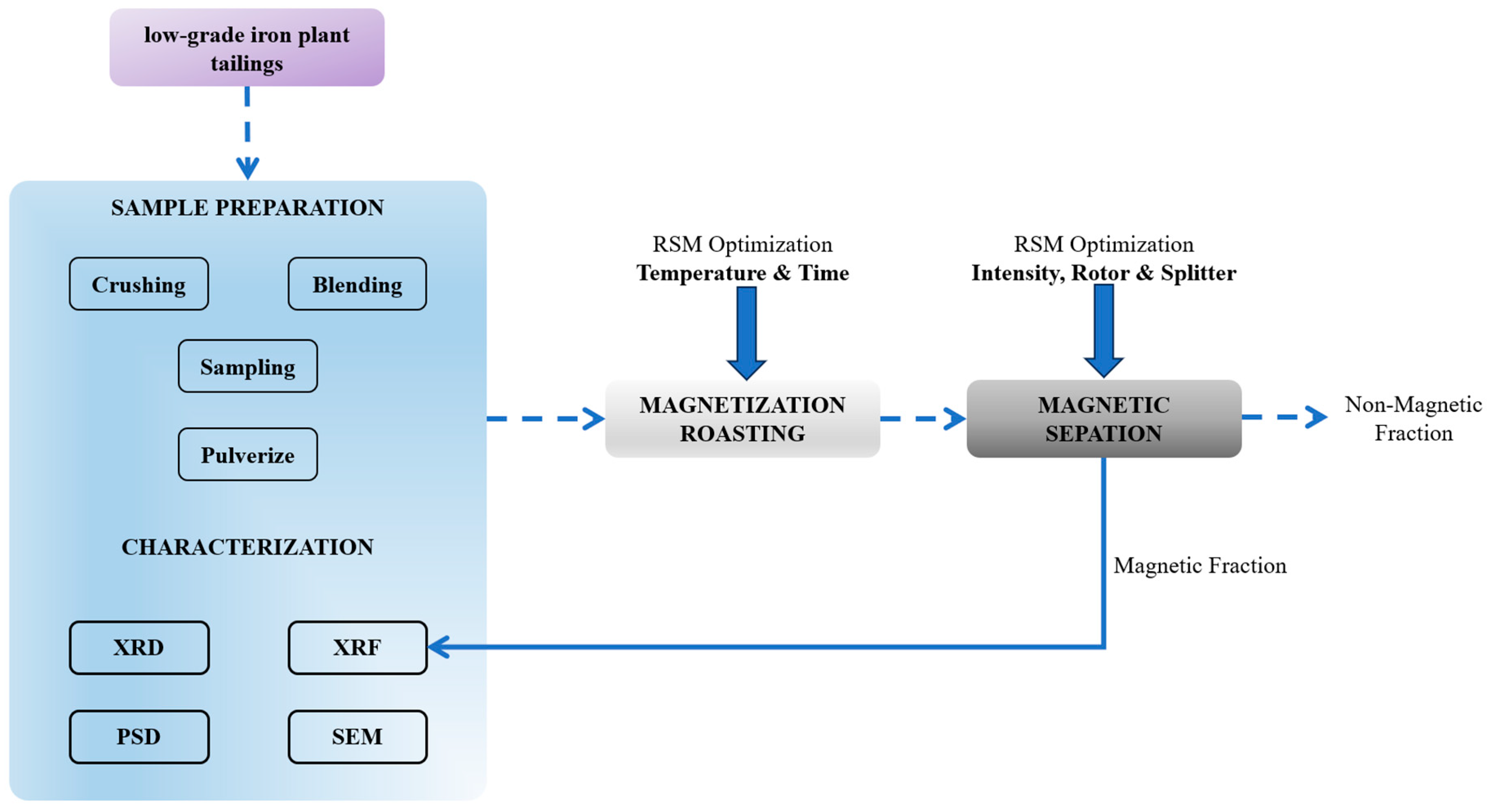
3.1. The As-Received Sample Characterization

The chemical composition of the sample, detailed in

Table 3. Chemical composition of the as-received sample.

Composition (%)
Fe	Na	Mg	Al	Si	S	Cl	K	Pb	Ca	Ti	Cr	Mn	O	Ca
57.1	0.02	0.03	2.18	5.11	0.04	0.01	0.71	0.10	0.08	0.09	0.02	0.57	34.04	0.08

, reveals that the head sample contains 82.76% Fe₂O₃, corresponding to a total iron (Fe) of 57.1%. Although the iron concentration in the iron plant tailings is substantial, it cannot be utilized directly for economic purposes due to significant impurities. The sample contains approximately 4.1% Al₂O₃ (2.2% Al) and 10.9% SiO₂ (5.11% Si). The assigned objective was upgrading the material to achieve at least 65% Fe. Additionally, the combined average of Al₂O₃ and SiO₂ must not exceed 5% to satisfy the required market specifications.

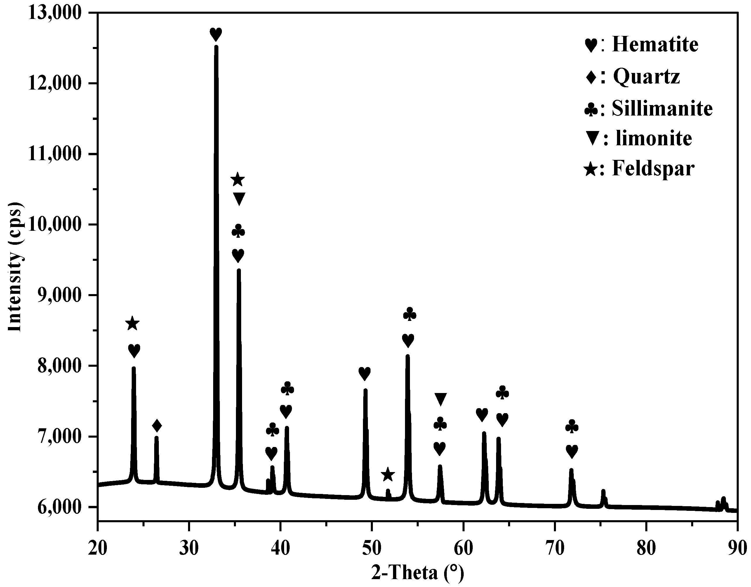
The analysis of the XRD spectrum for the iron tailings sample, as shown in Figure 2, revealed that the sample was dominated by the presence of Hematite occurring with traces of limonite characterized by paramagnetic behavior. Further examination indicated that Si, Al, and other elements were found in the form of quartz (SiO₂), sillimanite (Al₂SiO₅), and traces of feldspar (Na, K, Ca), Al (Al, Si)₃O₈. According to Srivastava et al. (2001) [12], quartz and sillimanite can result in a high slag volume, which may lead to the formation of viscous slag during the iron-making process. Therefore, it is crucial to reduce these impurities through beneficiation to enhance the productivity of iron-making operations.

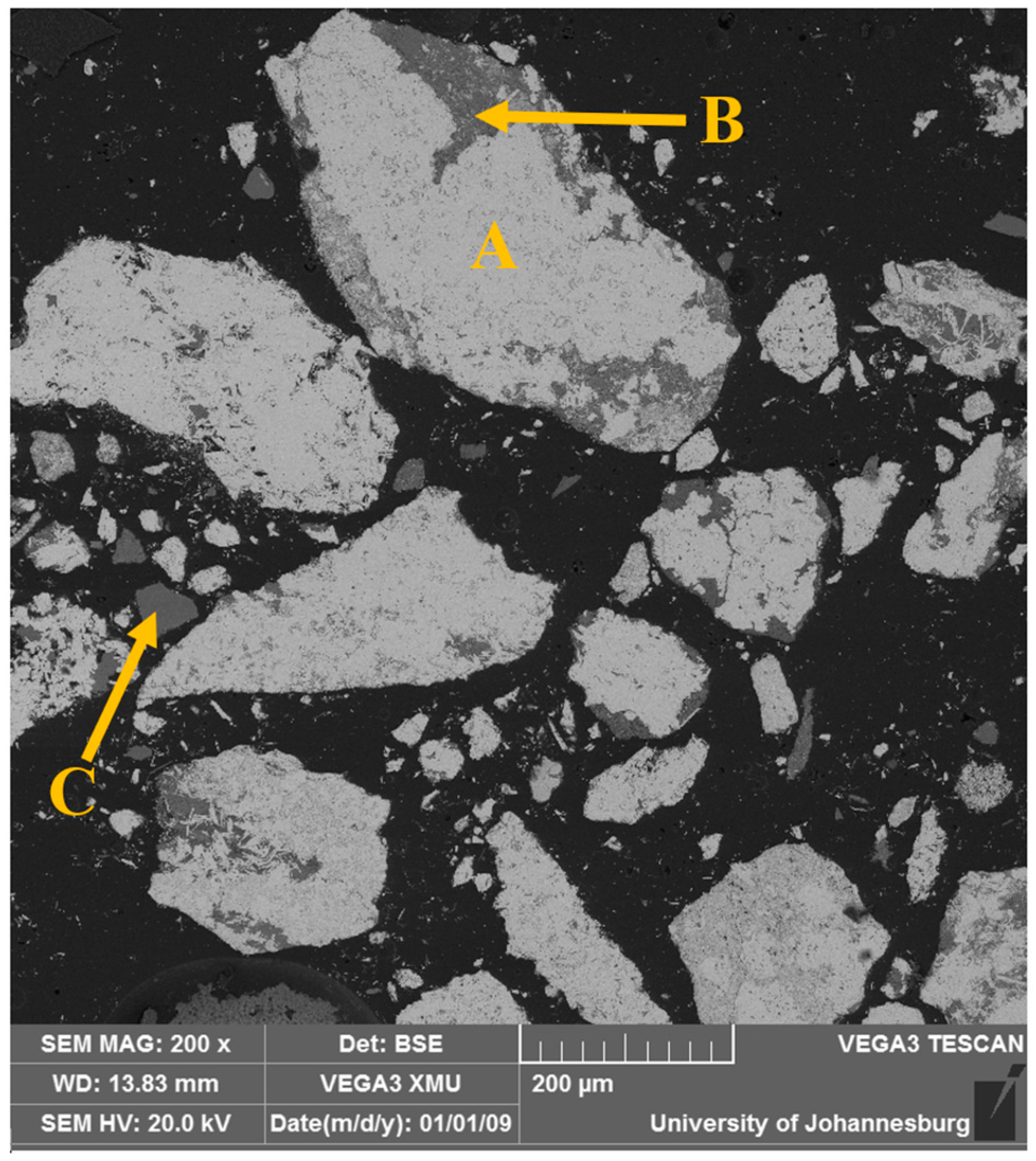
The morphology of the as-received sample was analyzed using SEM, while the chemical composition of the selected areas was determined using EDS. The micrograph results are shown in Figure 3, and the EDS spectra analysis results are provided in

Table 4. EDS result of the spectra of the as-received sample.

Spectrum	Composition (%)							Probable Phases
	O	Al	Si	K	Mn	Fe	Mg
A	63.46	0.00	0.69	0.00	0.00	35.84	0.00	Hematite
B	73.95	7.98	11.38	0.78	0.00	4.72	0.00	Quartz, Sillimanite
C	62.09	13.36	17.09	3.54	0.13	3.34	0.13	Quartz, Sillimanite

. The micrograph indicates that the sample is characterized by two main contrasts, indicating that the hematite phase (light gray) is interlocked into the silicate one (dark gray) and vice versa. It should be noted that the occurrence of the magnetite makes separation challenging. Therefore, a fine milling process was required to liberate Fe phases.

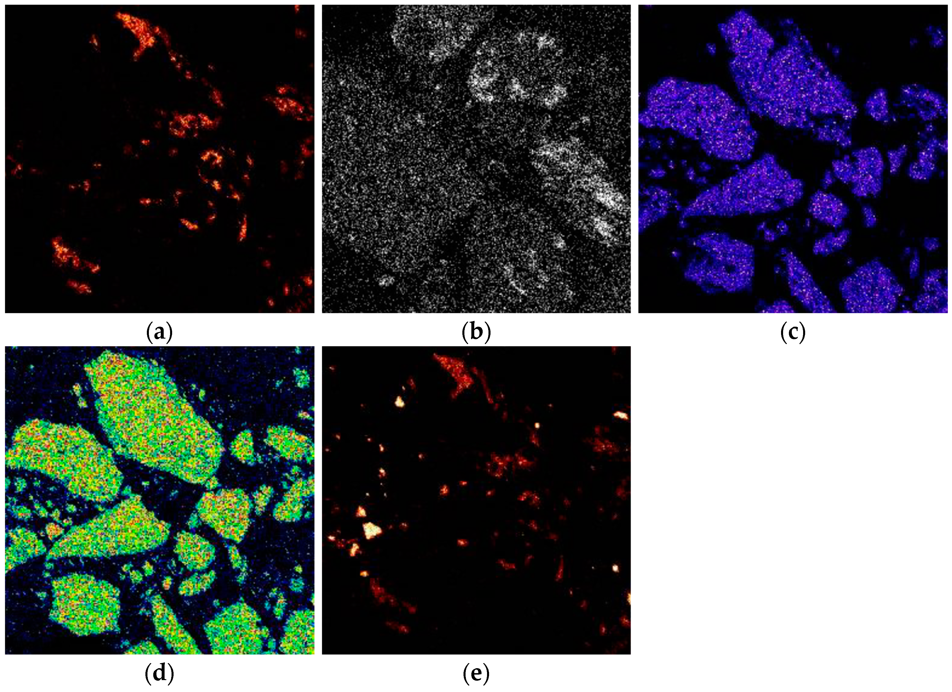
The bright spots that indicate heavier compounds are identified as Fe₂O₃, whereas the gray spots, predominantly composed of lighter compounds, reveal the presence of minerals such as quartz and sillimanite. The EDS analysis confirmed that the sample primarily comprises hematite, sillimanite, and quartz, consistent with the XRD results. Furthermore, it was noted that silica is distributed throughout the hematite matrix. The circled areas in the mapping, as shown in Figure 4, confirm the evidence of the interlinked Al-, Fe-, K-, and Si-bearing minerals.

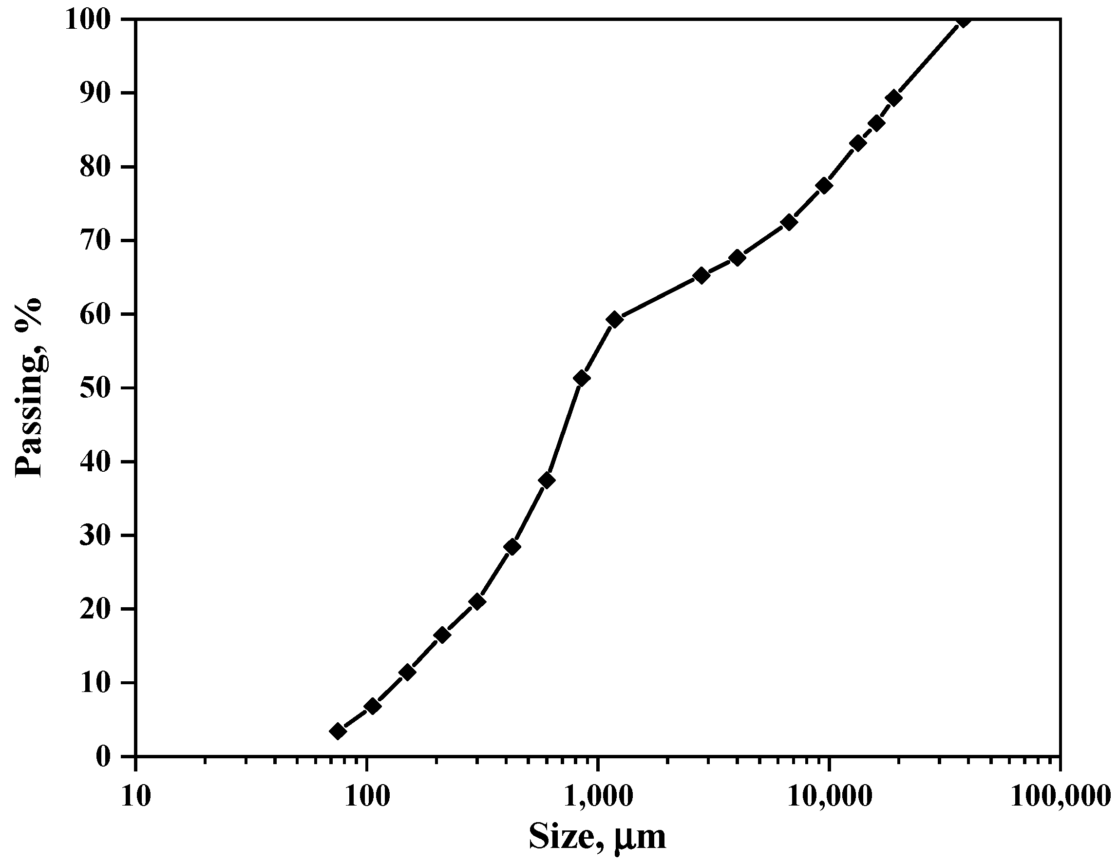
The particle size distribution of the as-received iron plant tailings was analyzed using wire mesh sieves, and the results are illustrated in Figure 5. The size distribution curve exhibits a bimodal profile, with sections covering the size ranges of 40,000–1180 µm and 1180–75 µm, corresponding to 40% and 60% splits, respectively. This suggests that the iron plant tailing sample originates from a processing route that employs various beneficiation techniques with different size specifications, similar to those described by Das and Rath (2020) [29]. The analysis further indicated that the F₈₀ of the iron tailing sample was 11,300 µm, encompassing a wide range of size fractions from 75 to 4000 µm, which points to a mixture of fine and coarse particles. Given that the primary objective of this project involves magnetic separation, it is crucial to compare the size distribution results of the as-received sample with the recommended particle size distribution for the effective operation of an induced dry-roll magnetic separator. This optimal range lies between 100 µm and 3000 µm, as Wills and Napier-Munn (2006) [30] specified. Therefore, the iron plant tailings must undergo comminution before processing to conform to these specifications.

3.2. Magnetic Susceptibility Test Results

The magnetic susceptibility test was performed on the un-roasted and roasted samples to evaluate the achievement of the transformation by applying the magnetic separation and comparing the Fe grades. The results presented in Figure 6 reveal that the grade of Fe in the concentrate of the unroasted sample was 61.8%. However, the determination of the Fe grade on the magnetized sample subjected to the same conditions of magnetic separation was found to be 66.1% as a sign of the ferrimagnetic material formation.

3.3. Optimization of the Magnetization Roasting Process Parameters

A two-factor five-level RSM optimal design was employed to assess the significance of roasting temperature (A) and time (B) and their interactions on the Fe grade and recovery achieved through magnetization roasting. A total of 12 experimental runs were proposed using Design-Expert^® software version 13.0.5.0.

Table 5. Experimental plan of optimal design with observed values for magnetization roasting optimization.

Run	Variables		Responses
	A: Roasting Temperature (°C)	B: Roasting Time (min)	Fe Grade (%)	Fe Recovery (%)
1	500	15	61.91	11.47
2	1100	60	64.45	16.09
3	500	90	65.03	8.87
4	800	60	66.23	16.34
5	800	120	66.75	16.27
6	1100	15	65.92	16.27
7	650	30	62.11	15.9
8	1100	90	65.84	16.07
9	800	15	64.13	15.77
10	800	60	66.23	16.34
11	500	60	64.71	8.23
12	500	120	65.55	9.32

presents an overview of the experimental design and the observed responses for optimizing magnetization roasting.

Two statistical models were developed for each response variable, i.e., Fe grade and Fe recovery. A linear first-order model was utilized to represent the relationship between Fe grade and each input factor derived from the experimental data [31]. Conversely, a quadratic second-order polynomial model described the relationship between controllable variables and Fe grade and recovery. The empirical coded equations for the Fe grade and Fe recovery are shown in Equations (4) and (5), respectively.

Fe grade (%) = 65.19 + 0.92 A + 1.41 B

(4)

Fe recovery (%) = 16.05 + 3.31 A − 0.3 B + 0.83 A × B − 3.46 A² + 0.75 B²

(5)

where the Fe grade and recovery are given in percentage, roasting temperature (A) is in °C, and roasting time (B) is in minutes.

The analysis of variance (ANOVA) was utilized at a 5% significant level to validate the adequacy of the developed regression models for Fe grade and recovery for a p-value ≤ 0.05.

Table 6. ANOVA analysis for Fe grade in the magnetization roasting.

Source	Sum of Squares	DF	Mean Square	F-Value	p-Value	Remark
Model	15.32	2	7.66	5.96	0.0225	significant
A—Temperature	5.83	1	5.83	4.54	0.062	not significant
B—Time	11.32	1	11.32	8.81	0.0158	significant
Residual	11.56	9	1.28
Cor Total	26.88	11
Adeq precision: 6.7872

and

Table 7. ANOVA analysis for Fe recovery in the magnetization roasting.

Source	Sum of Squares	DF	Mean Square	F-Value	p-Value	Remark
Model	118.46	5	23.69	23.64	0.0007	significant
A—Temperature	70.30	1	70.30	70.13	0.0002	significant
B—Time	0.4480	1	0.4480	0.4470	0.5286	not significant
A × B	1.91	1	1.91	1.91	0.2163	not significant
A2	30.84	1	30.84	30.77	0.0015	significant
B2	1.19	1	1.19	1.19	0.3175	not significant
Residual	6.01	6	1.00
Cor Total	124.47	11
Adeq precision: 11.6

present the ANOVA analysis conducted for Fe grade and Fe recovery during the magnetization roasting optimization.

Table 6 shows that a fissure test value (F-value) of 5.96 implies that the Fe grade model is significant. There is only a 2.25% chance that an F-value this large could occur due to noise.

The value of Adequate Precision (Adeq Precision) serves as a signal-to-noise ratio to evaluate the sufficiency of a model. Two hypotheses were formulated to assess the sufficiency [32].

• The “null hypotheses—H₀” suggests that the “Adeq Precision” value is >4: the predicted model fits the data and indicates adequate model discrimination.
• The “alternate hypotheses—H_a” implies that the value of “Adeq Precision” is <4, suggesting that the predicted model does not adequately fit the data and exhibits insufficient model discrimination.

With an “Adeq Precision” ANOVA value of 6.7872, which exceeds 4, we can conclude that the model is sufficient and can be reliably used to navigate the design space [33].

The values of p-values below 0.05 indicate that the model terms are statistically significant. In the context of Fe grade, the results reveal that term B is significant. The F-value assesses the main effects and their interactions, with larger F-values indicating greater significance. The order of significance for the main effects related to Fe grade was determined to be B > A.

Table 7 shows that the F-value of 23.64 signifies the significance of the Fe recovery model, with only a 0.07% probability that such a large F-value could arise from random noise. Additionally, the “Adeq Precision” ANOVA value of 11.6 exceeds 4, demonstrating that the model is sufficient for navigating the design space.

The analysis indicated that the terms A and A² were significant in the Fe recovery model (p-value < 0.05). According to the F-value, the order of significance for the main effects and interactions influencing Fe recovery is as follows: A > A² > A × B > B² > B.

The comparison of actual and predicted Fe grade and recovery values is derived from the regression model Equations (4) and (5), which are presented in

Table 8. Actual and predicted values of Fe grade and Fe recovery in the magnetization roasting optimization.

Run	Fe Grade (%)		Fe Recovery (%)
	Actual	Predicted	Actual	Predicted
1	61.91	62.86	11.47	11.16
2	64.45	65.90	16.09	15.85
3	65.03	64.88	8.87	8.93
4	66.23	64.99	16.34	16.11
5	66.75	66.60	16.27	16.50
6	65.92	64.69	16.27	16.13
7	62.11	63.72	15.90	14.43
8	65.84	66.71	16.07	16.27
9	64.13	63.78	15.77	17.11
10	66.23	64.99	16.34	16.11
11	64.71	64.07	8.23	9.46
12	65.55	65.68	9.32	8.89

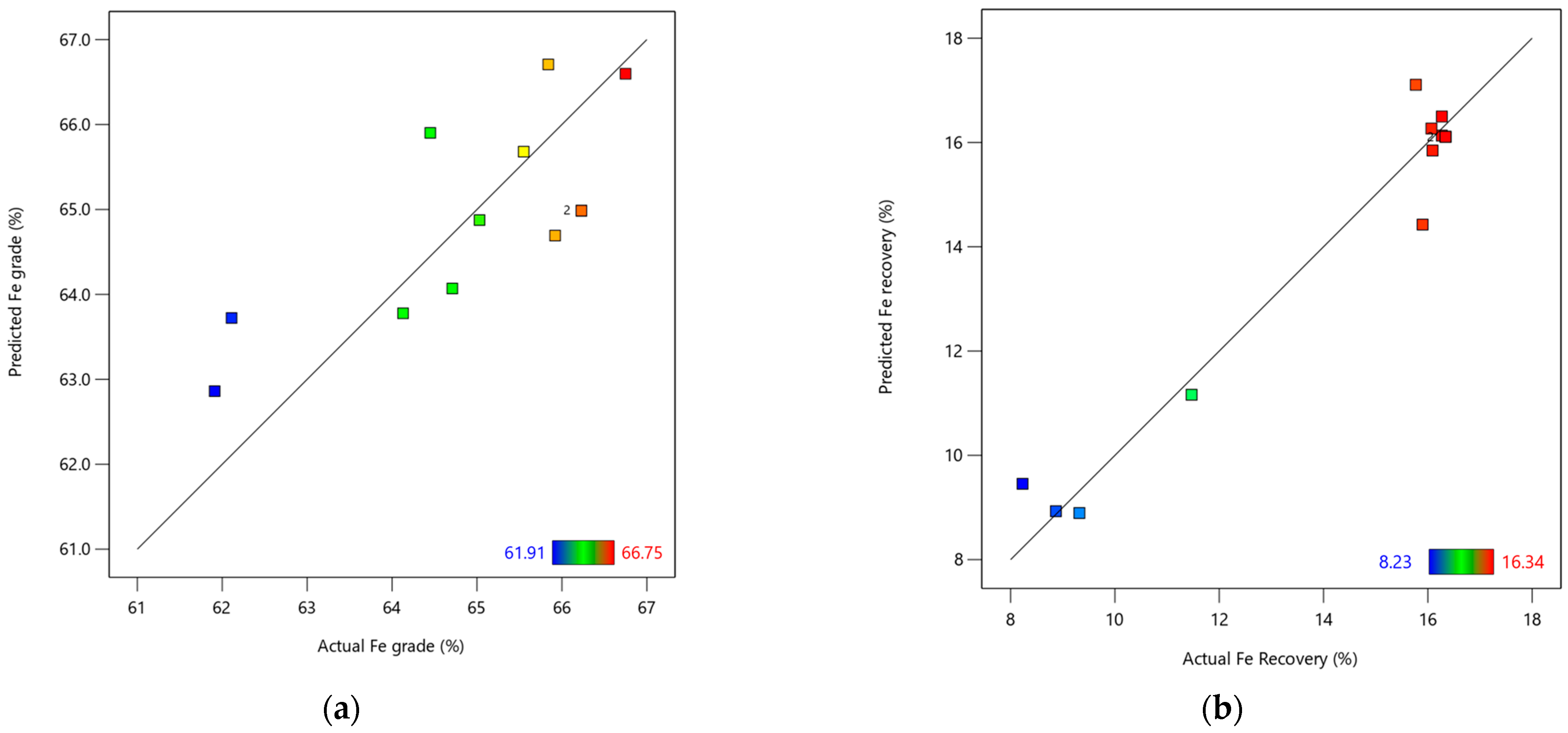
. Figure 7a,b also illustrates the relationship between the actual and predicted Fe grade and recovery, respectively.

According to Figure 7a, a moderately good fit was observed between the actual and predicted Fe, with a correlation R² value of 0.56. However, additional investigations may be necessary to refine the regression model. In contrast, Figure 7b illustrates a strong correlation between the actual and predicted values of Fe recovery, as evidenced by an R² value of 0.95. This indicates that the developed iron recovery model is effective and reliable.

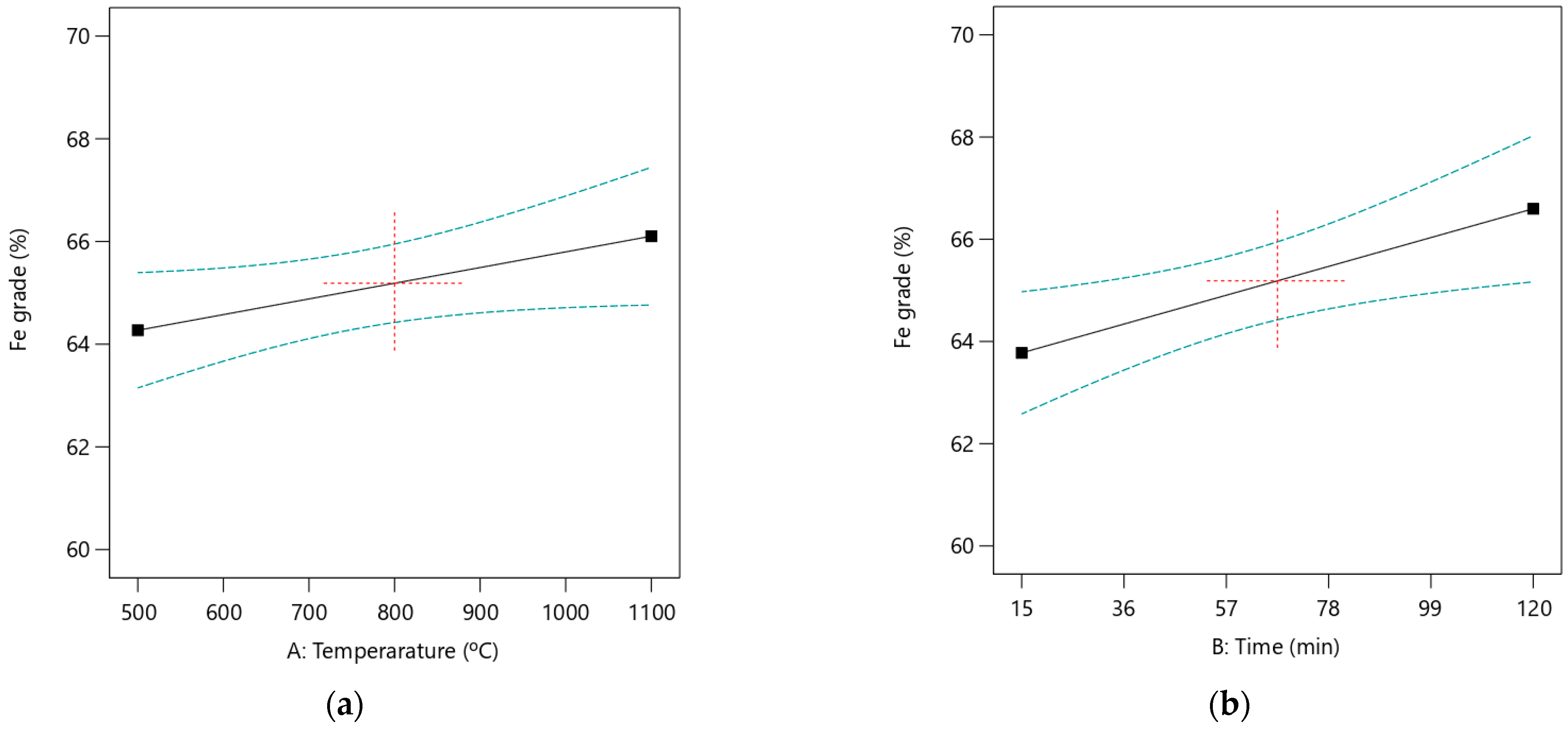
The steep slope observed in Figure 8 indicates a more substantial influence of the main effect on the Fe grade, as previously predicted with the ANOVA analysis. Furthermore, based on a first-order linear model developed for Fe grade, there is no evidence of a two-way interaction between the input factors affecting Fe grade.

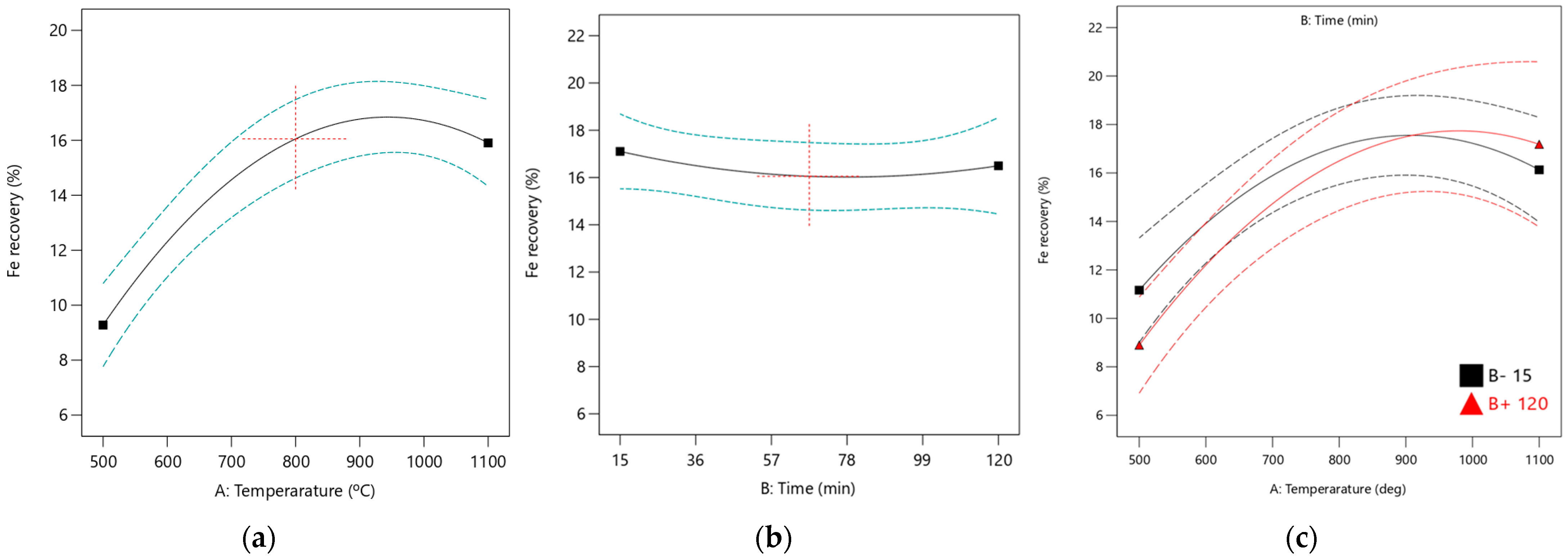
It was observed that the roasting time is nearly parallel to the horizontal axis, as illustrated in Figure 9b. This indicates that the effect of roasting time on Fe recovery is minimal and consistent with the predictions made with the ANOVA analysis. The interaction plot between roasting temperature and time, also shown in Figure 9c, evaluates the effects of these independent factors. Increasing the roasting temperature improves Fe recovery, irrespective of whether the roasting time is high or low. However, the interaction between roasting temperature and time has a low impact on Fe recovery, as indicated by the ANOVA results. The quadratic effects of temperature and time were not significant, reflected in their low F-values.

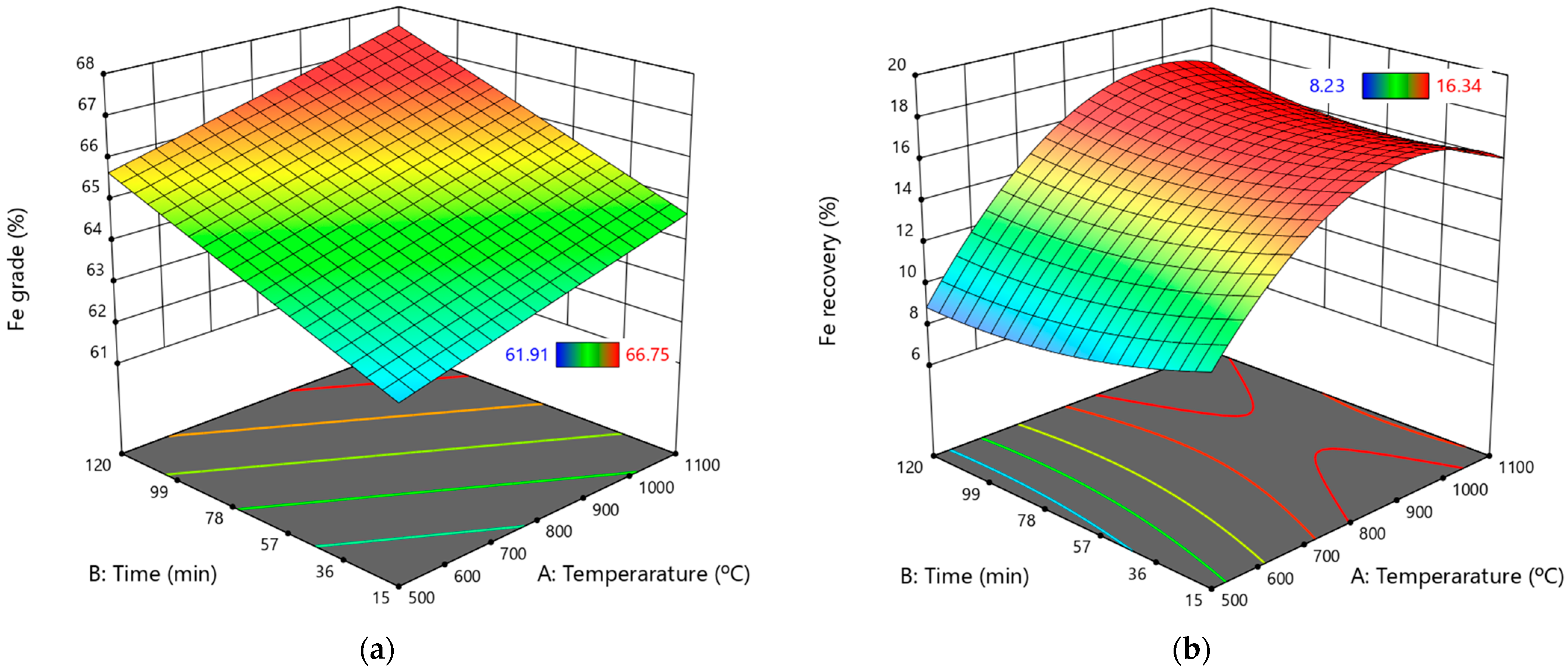
Three-dimensional response surface and contour plots are essential for comprehending the main and interaction effects of the independent factors. These plots can support decision-making in selecting suitable input conditions to yield the optimal combination for the target response [14,33,34]. The combined contour and 3D surface plots, which display the interactions of the variables on Fe grade and Fe recovery, are presented in Figure 10a,b.

Utilizing the findings illustrated in Figure 10a,b, the optimum working zone (optimized formulation region) can be easily identified [35]. Figure 10a illustrates that the Fe grade increases with the roasting temperature and time. In contrast, the 3D surface plot regarding Fe recovery indicates that only increased roasting temperature has a positive effect, while additional roasting time does not contribute to improved recovery. Therefore, a shorter roasting time that does not compromise the Fe grade can be chosen to save production time and costs.

In mineral processing, grade and recovery are essential parameters for evaluating the performance of any unit process. As such, the model responses were optimized using the Design-Expert^® prediction profiler. During the magnetization roasting process, the optimization aimed to achieve a maximum Fe grade of at least 65%, which is crucial for economic viability.

Table 9. Response prediction for the Fe grade and Fe recovery in the magnetization roasting.

Desirability	Variable		Response
	A: Temperature (°C)	B: Time (min)	Fe Grade (%)	Fe Recovery (%)
1.000	1050	98	66.76	16.80

summarizes the optimal solution values for variables calculated by the model to achieve the desired Fe grade and Fe recovery. In this context, the desirability function uses a value of “0” to represent an undesirable response and a value of “1” to indicate the most ideal and desirable response.

The results in Table 9 indicate that operating at optimal roasting temperatures of 1050 °C and a duration of 67 min yields an Fe grade of 66.8%, but only results in a recovery rate of 16.9%. Notably, these roasting conditions lead to the lowest levels of Fe recovery. Therefore, optimizing the next stage, which involves the induced dry-roll magnetic separator, is crucial.

The optimized operating conditions were used to assess the suitability of the developed model in predicting response values. To validate these optimal conditions, an experiment was conducted, resulting in an Fe recovery rate of 17.63% at an Fe grade of 67.45%. The experimental response values aligned well with the predicted values, as illustrated in Table 9. The model is reliable and accurate in forecasting outcomes.

3.4. Optimization of the Induced Dry-Roll Magnetic Separator Process Parameters

The sample generated at the optimum roasting temperature of 1050 °C and a roasting time of 98 min was used to prepare a bulk material for optimizing the induced dry-roll magnetic separation. RSM was also utilized to evaluate the influence of magnetic field intensity (A), rotor speed (B), and product splitter position (C) on iron (Fe) grade and Fe recovery. After conducting the experiments, the outcomes of the experimental design and the observed responses for optimizing induced dry-roll magnetic separation are presented in

Table 10. Experimental plan of optimal design with observed values for induced dry-roll magnetic separator optimization.

Run	Variables			Responses
	A: Magnetic Field Intensity (T)	B: Rotor Speed (Hz)	C: Product Splitter Position (mm)	Fe Grade (%)	Fe Recovery (%)
1	0.14	70	5	64.99	41.22
2	0.1	70	15	65.53	47.88
3	0.1	40	10	66.37	37.73
4	0.14	60	15	66.35	31.87
5	0.14	20	10	65.06	11.54
6	0.1	70	10	65.84	67.93
7	0.1	70	10	65.82	67.97
8	0.1	40	10	66.38	37.72
9	0.05	40	10	65.31	48.86
10	0.05	70	10	65.61	64.49
11	0.14	60	10	66.1	37.37
12	0.05	20	15	66.53	15.8
13	0.1	20	15	64.98	12.73
14	0.14	20	10	65.09	11.55
15	0.05	70	15	65.17	54.4
16	0.1	40	5	64.81	41.78
17	0.05	20	5	66.3	20.82
18	0.1	40	5	64.84	41.79
19	0.1	40	10	66.37	37.73
20	0.05	70	5	64.12	69.98

.

Two statistical models were developed for each response: Fe grade and Fe recovery. A quadratic second-order polynomial was used to describe the relationship between the input factors and the output responses. The empirical coded equations for both Fe grade and Fe recovery are provided in Equations (6) and (7), respectively.

Fe grade (%) = 66.02 − 0.15 A − 0.07 B + 0.37 C + 0.72 A × B + 0.01 A × C
+ 0.24 B × C – 0.02 A² − 0.06 B² − 0.72 C²

(6)

Fe recovery (%) = 46.33 − 9.41 A + 19.77 B − 4.74 C − 1.96 A × B + 1.52 A × C
− 1.49 B × C − 7.28 A² − 1.59 B² − 6.45 C²

(7)

where the Fe grade and recovery are given in percentage, magnetic field intensity (A) is in T, rotor speed (B) is in Hz, and product splitter position (C) is in mm.

The ANOVA analysis was utilized at a 5% significance level to evaluate the adequacy of the developed polynomial regression models for Fe grade and Fe recovery, in which the significance was determined for p-values ≤ 1.

Table 11. ANOVA analysis for Fe grade in the induced dry-roll magnetic separation.

Source	Sum of Squares	DF	Mean Square	F-Value	p-Value	Remark
Model	6.99	9	0.7764	3.80	0.0246	Significant
A—Field intensity	0.2285	1	0.2285	1.12	0.3154	not significant
B—Rotor Speed	0.0651	1	0.0651	0.3183	0.5851	not significant
C—Splitter position	1.18	1	1.18	5.77	0.0372	significant
A × B	3.83	1	3.83	18.71	0.0015	significant
A × C	0.0531	1	0.0531	0.2594	0.6216	not significant
B × C	0.3751	1	0.3751	1.83	0.2055	not significant
A2	0.0014	1	0.0014	0.0070	0.9348	not significant
B2	0.0103	1	0.0103	0.0502	0.8273	not significant
C2	2.10	1	2.10	10.27	0.0094	significant
Residual	2.05	10	0.2045
Cor Total	9.03	19
Adeq Precision: 7.03

and

Table 12. ANOVA analysis for Fe recovery in the induced dry-roll magnetic separation.

Source	Sum of Squares	DF	Mean Square	F-Value	p-Value	Remark
Model	6638.10	9	737.57	40.16	<0.0001	significant
A—Field intensity	901.54	1	901.54	49.08	<0.0001	significant
B—Rotor Speed	4660.62	1	4660.62	253.74	<0.0001	significant
C—Splitter position	194.15	1	194.15	10.57	0.0087	significant
A × B	28.35	1	28.35	1.54	0.2424	not significant
A × C	12.37	1	12.37	0.6733	0.4310	not significant
B × C	13.92	1	13.92	0.7581	0.4044	not significant
A2	215.41	1	215.41	11.73	0.0065	significant
B2	6.72	1	6.72	0.3657	0.5588	not significant
C2	167.49	1	167.49	9.12	0.0129	significant
Residual	183.68	10	18.37
Cor Total	6821.77	19
Adeq Precision: 19.69

present the ANOVA analysis for Fe grade and recovery, respectively. As shown in Table 11, the F-value of 3.8 indicates that the Fe grade model is statistically significant, with only a 2.46% probability that such an F-value could arise from random noise. Additionally, the “Adeq Precision” ANOVA value of 7.03 exceeds the threshold of 4, suggesting that the model is sufficient and can be effectively used to explore the design space.

The significant factors affecting Fe grade were C, A × B, and C² (p-value < 0.05). Based on the F-values, the order of significance for the main and interaction effects on Fe grade is as follows: A × B > C² > C > B × C > A > B > A × C > B² > A².

The results from Table 12 indicate that the F-value of 40.16 demonstrates the significance of the developed model for Fe recovery. There is only a 0.01% chance that an F-value this high could occur due to random noise. Furthermore, the “Adeq Precision” ANOVA value of 19.69 surpasses the threshold of 4, confirming that the model is adequate and can effectively guide the design space.

The analysis revealed that the terms A, B, C, A², and C² are significant (p-value < 0.05). The order of significance of the main and interaction effects was B > A > A² > C > C² > A × B > A × C > B × C > B².

The actual and predicted Fe grade and Fe recovery values were compared using the quadratic polynomial Equations (6) and (7), which are given in

Table 13. Actual and predicted values of Fe grade and Fe recovery in the induced dry-roll magnetic separator optimization.

Run	Fe Grade (%)		Fe Recovery (%)
	Actual	Predicted	Actual	Predicted
1	64.99	65.00	41.22	44.12
2	65.53	65.85	47.88	50.65
3	66.37	65.99	37.73	41.22
4	66.35	66.11	31.87	29.19
5	65.06	65.14	11.54	10.24
6	65.84	65.94	67.93	63.16
7	65.82	65.94	67.97	63.16
8	66.38	65.99	37.72	41.22
9	65.31	66.30	48.86	44.05
10	65.61	65.29	64.49	68.61
11	66.10	66.21	37.37	39.75
12	66.53	66.18	15.80	13.91
13	64.98	65.34	12.73	14.52
14	65.09	65.14	11.55	10.24
15	65.17	65.08	54.40	54.41
16	64.81	64.94	41.78	39.05
17	66.30	66.13	20.82	23.47
18	64.84	64.94	41.79	39.05
19	66.37	65.99	37.73	41.22
20	64.12	64.05	69.98	69.91

. Figure 11a,b illustrates the relationships between the actual and predicted Fe grade and Fe recovery, respectively.

Figure 11a indicates a good fit between the actual and predicted Fe grade values, as evidenced by an R² value of 0.77. Meanwhile, Figure 11b suggests a strong correlation between the predicted and experimental data for Fe recovery. This indicates that the Fe grade and recovery models are effective and reliable.

However, it is essential to note that one data point (run 8) in the Fe grade analysis lies outside the acceptable range, indicating a residual more significant than 4. This suggests that run 8 is an outlier, and repeating this run could enhance the model’s accuracy.

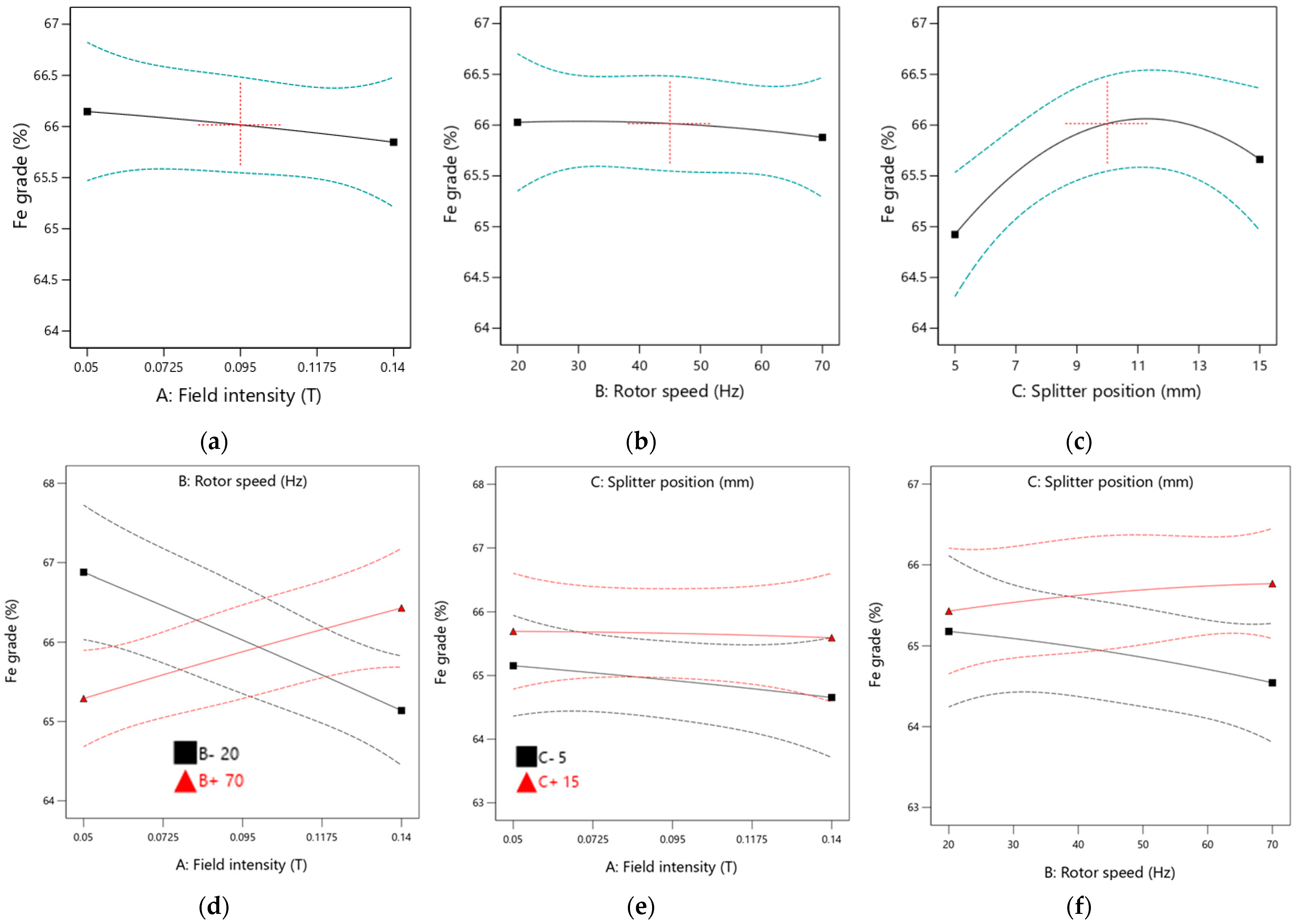
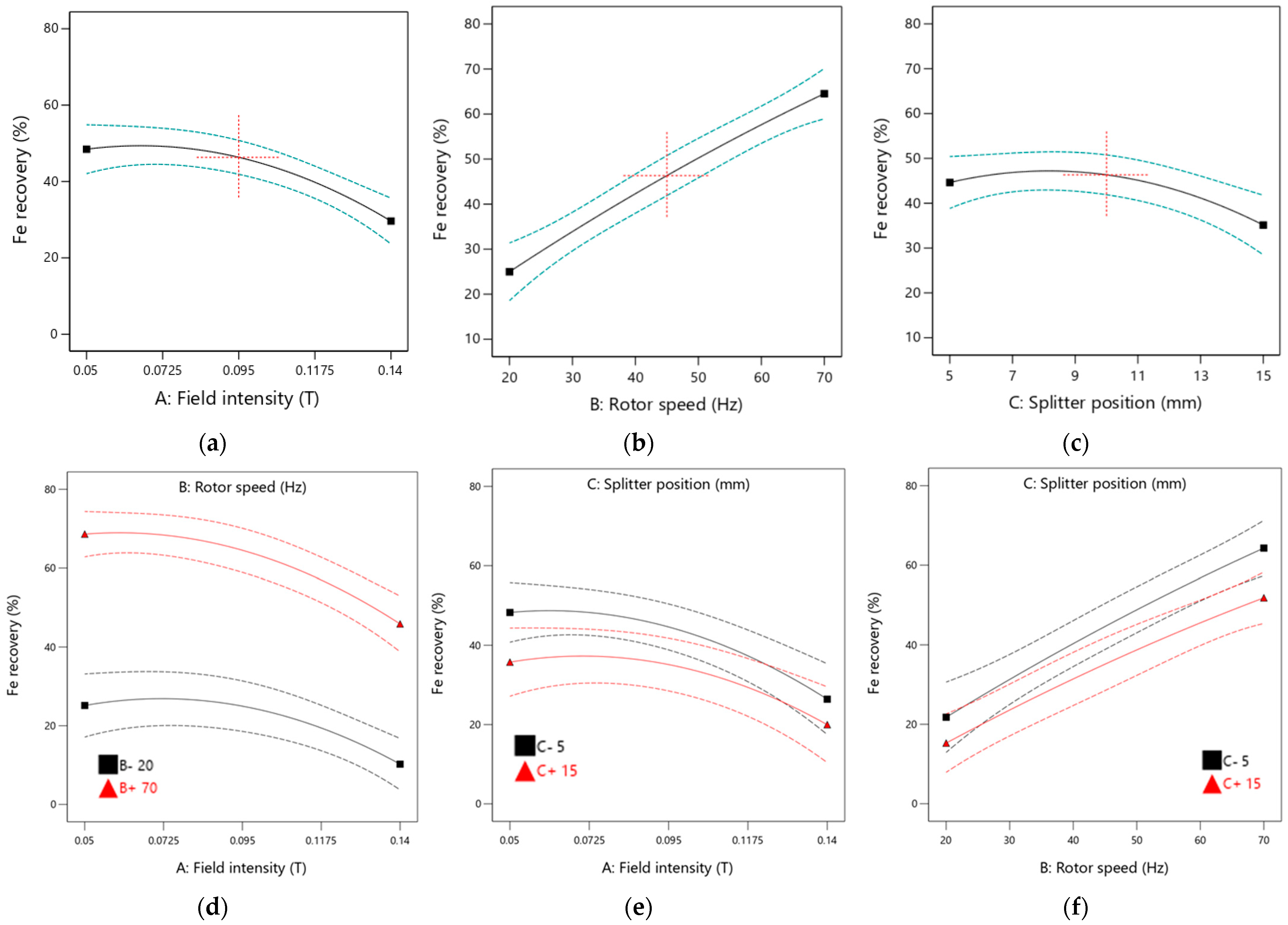
The main and interaction effect plots were developed to illustrate the relationship between the input parameters (magnetic field intensity, rotor speed, and product splitter position) and the output parameters (Fe grade and Fe recovery). The generated plots are presented in Figure 12 and Figure 13 for Fe grade and Fe recovery, respectively.

The results indicate that the product splitter position positively impacts the obtained Fe grade, as evidenced by the steep slopes observed in the main plot for the splitter position. In contrast, the main plots for magnetic field intensity and rotor speed are nearly parallel to the horizontal axis, suggesting that increases in these parameters have an insignificant effect on the Fe grade. This aligns with the ANOVA analysis, which found the p-values for field intensity and rotor speed to be insignificant.

The interaction effects involving field intensity and rotor speed, field intensity and splitter position, and rotor speed and splitter position on Fe grade are illustrated in Figure 12. It was observed that the Fe grade increases only with higher field intensity and rotor speed. Lower rotor speeds resulted in poor Fe grades. The interaction between field intensity and splitter position contributed minimally to the Fe grade, as indicated by a plot that is parallel to the horizontal axis. However, operating the equipment at a higher splitter position leads to better Fe grades. Additionally, increasing rotor speed while using a lower splitter position negatively affects the Fe grade. The interactions between field intensity and splitter position and those between rotor speed and splitter position demonstrate minimal impact on the Fe grade due to low F-values, as shown in the ANOVA analysis.

Based on Figure 13, field intensity and rotor speed positively influence Fe recovery, as indicated by the steep slopes in the main effect plots. The Fe recovery increases with higher rotor speeds, while an increase in field intensity has a negative impact on recovery, suggesting that optimal results are achieved at lower field intensities. The main plot for the splitter position remains nearly parallel to the horizontal axis, indicating that adjustments to the splitter position have minimal effect on Fe recovery. This observation is consistent with the ANOVA analysis, which reveals a low F-value for the splitter position.

Interaction effect plots for field intensity and rotor speed, field intensity and splitter position, and rotor speed and splitter position on Fe recovery are shown in Figure 13. It is noted that increasing field intensity adversely affects Fe recovery. However, operating the equipment at lower field intensity and rotor speed produces better Fe recoveries. Operating the equipment at a lower rotor speed is not advisable, resulting in significantly lower Fe recovery. The interaction between field intensity and splitter position has a moderate effect on Fe recovery, with optimal conditions identified as low field intensity and low splitter position. Increasing rotor speed while maintaining a lower splitter position enhances Fe recovery values. Nonetheless, all interaction effects have minimal influence on Fe recovery, as indicated by low F-values, with all corresponding p-values exceeding 0.05, which aligns with the ANOVA analysis data.

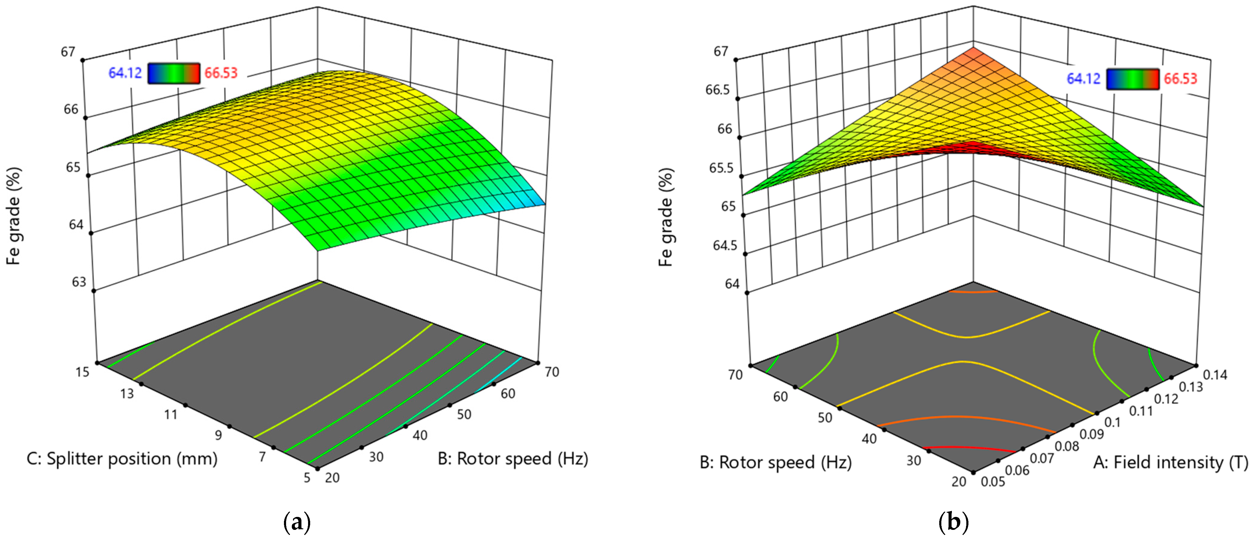
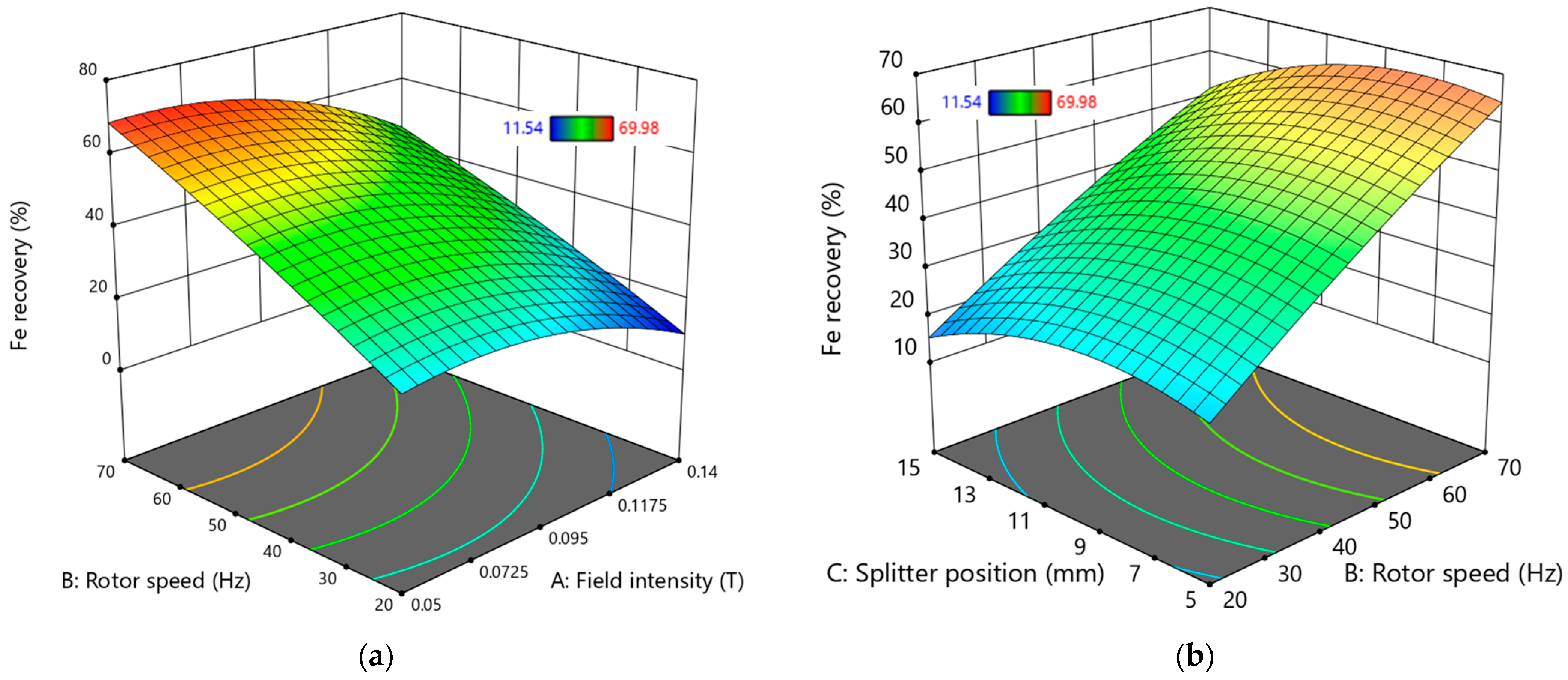
The 3D surface plots illustrating the interactions of variables affecting Fe grade and Fe recovery are presented in Figure 14 and Figure 15.

According to Figure 14a, the range that promotes a higher Fe grade is found with a splitter position between 10 mm and 11.5 mm at any rotor speed. However, selecting a lower rotor speed is advisable for economic reasons, as it can reduce energy costs. This is further supported by Figure 14b, which indicates that operating the equipment at a low rotor speed and in a lower field intensity region yields optimal Fe grade values.

In Figure 15a, the conditions for improved Fe recovery are highlighted, showing that a high rotor speed above 65 Hz is necessary while maintaining a field intensity of less than 0.09 T. Figure 15b reveals that, for higher Fe recovery values, the product splitter position should be set below 11 mm at rotor speeds exceeding 65 Hz.

Table 14. Response prediction for the Fe grade and Fe recovery in the induced dry-roll magnetic separation.

Desirability	Variable			Response
	A: Field Intensity (T)	B: Rotor Speed (Hz)	C: Splitter Position (mm)	Fe Grade (%)	Fe Recovery (%)
0.828	0.105	70	11	66.10	60.20

presents the best solutions for the variables necessary to achieve the desired Fe grade and recovery. Based on Table 14, the optimum working conditions include a magnetic field intensity of 0.105 T, a rotor speed of 70 Hz, and a product splitter position of 11 mm, resulting in an Fe grade of 66.2% and a recovery rate of 60.2%.

To validate these optimal conditions, an experiment was conducted, resulting in an Fe recovery rate of 58.29% and an Fe grade of 65.33%. The experimental response values aligned well with the predicted values, as shown in Table 14.

4. Conclusions

The development and optimization of procedures are essential steps in analytical methods. This study aimed to establish optimized working conditions for magnetization roasting and induced dry-roll magnetic separation to achieve the desired Fe grade and recovery. The RSM was employed to model and optimize various operational parameters based on a selected optimal design configuration. The statistical model predicted a satisfactory Fe grade of 66.76%, an increase from an initial 57.1%, with an Fe recovery of 16.7%. This was achieved at a roasting temperature of 1050 °C over 97 min during the magnetization roasting optimization. However, the Fe recovery was notably low, highlighting the need to optimize the induced dry-roll magnetic separator. For the induced dry-roll magnetic separator, the statistical model predicted an optimum Fe grade of 66.1% with an improved Fe recovery of 60.2%. The optimal working conditions were identified as a field intensity of 0.105 T, a rotor speed of 70 Hz, and a product splitter position of 11 mm. Based on the ANOVA analysis, it was found that the optimization of Fe grade during magnetization roasting was significantly influenced by roasting time.

In contrast, the impact of roasting temperature on Fe grade was less pronounced. However, the roasting temperature was crucial in achieving high Fe recovery during magnetization roasting. In the case of the induced dry-roll magnetic separator, only the product splitter position significantly impacted the Fe grade. In contrast, all parameters significantly affected the Fe recovery, with rotor speed having the most significant impact, followed by field intensity. Applying the RMS optimal design has led to developing a robust and reliable method for accurately determining the optimal operating conditions in magnetization roasting and induced dry-roll magnetic separation.

This study presents positive outcomes on the use of biomass as a reductant; however, challenges may arise when scaling this solution. Unlike coal or coke, biomass may struggle with issues of limited supply. Thus, it is essential to conduct further investigations into various agro-industrial biomass sources, such as corn straw, rice husks, sawdust, starch, macadamia nutshells, coconut shells, and cow dung, whether used individually or in combination. Furthermore, the model developed in this study can act as an initial framework for exploring the potential of biomass in these applications.