Article

Estimation of Copper Grade, Acid Consumption, and Moisture Content in Heap Leaching Using Extended and Unscented Kalman Filters

by
Lisbel Bárzaga-Martell
1,2,*,
Simón Diaz-Quezada
2,
Humberto Estay
2 and
Javier Ruiz-del-Solar
2,3
1
Department of Electricity, Universidad Tecnológica Metropolitana, Av. José Pedro Alessandri 1242, Ñuñoa, Santiago 7800002, Chile
2
Advanced Mining Technology Center, Universidad de Chile, Av. Tupper 2007, Santiago 8370451, Chile
3
Department of Electrical Engineering, Universidad de Chile, Av. Tupper 2007, Santiago 8370451, Chile
*
Author to whom correspondence should be addressed.
Minerals 2025, 15(5), 521; https://doi.org/10.3390/min15050521
Submission received: 24 March 2025 / Revised: 21 April 2025 / Accepted: 23 April 2025 / Published: 14 May 2025

Abstract

:
The leaching process is essential in the mining industry, because it efficiently extracts valuable minerals, such as copper. However, monitoring and controlling the leaching process presents significant challenges due to material variability, uneven distribution of the leaching solution, and the effects of environmental factors like temperature and moisture content. One of the main technological challenges is measuring variables within the leaching heap. Implementing state observers or estimators (i.e., virtual sensors) offers a promising solution, allowing for a cost-effective estimation of non-measurable process variables. To validate this approach, this paper proposes and analyzes the use of two estimation methods, the Extended Kalman Filter (EKF) and the Unscented Kalman Filter (UKF), to estimate the moisture content, copper in the ore, and acid consumption based on measurements of acid and copper concentrations in the heap leaching process. The results obtained from simulations demonstrate accurate estimations from both state observers. The variable best estimated with EKF was the moisture content, achieving a 0.041% Integral Absolute Error (IAE) and a 0.069% Integral Square Error (ISE) in one of the analyzed scenarios. Utilizing these state estimators improves the understanding of the internal dynamics of heap leaching, often limited by the lack of field-level instrumentation, such as sensors and transmitters. This approach can enhance the operational efficiency of heap leaching plants by enabling the real-time estimation of unmeasurable variables, ultimately improving metal recovery and reducing acid consumption.

1. Introduction

Heap leaching is an extraction method that dissolves desired components from solid minerals through a systematically irrigated liquid solvent (chemical extraction of minerals). Various leaching methods are available, such as heap leaching, in situ leaching, dump leaching, percolation leaching, and agitated leaching. Heap leaching entails the organized stacking of crushed and agglomerated minerals, aiming for cost-effective leaching processes [1].
While cost-effective, heap leaching presents unique process monitoring and control challenges. The heap leaching process can be modeled as a trickle bed reactor, where the hydrodynamics can describe an unsaturated bed flow. In addition, the dissolution occurs along the height of the heap, determining the changing values of different variables.
Furthermore, heap leaching processes typically produce particle sizes larger than 1/2” [2]. Due to these larger particle sizes, the leaching process is slower and requires a significant area to handle the processing rates of several thousand tons per day, often covering several hectares. This characteristic introduces complexities in the process control, such as determining suitable data transmission methods for the sensor data and the number of sensors required for specific variables. Moreover, measuring internal variables within the heap is not feasible, as it is not possible to install sensors inside the heap, adding further challenges to process monitoring and control [3].
Nevertheless, it is possible to perform certain indirect measurements in heap leaching. For example, thermal cameras mounted on drones have been successfully employed to estimate the heap’s surface temperature relative to the surrounding environment [4]. However, directly measuring internal variables such as the moisture content remains unfeasible. An innovative approach explored by Tang et al. [5] combined drone-based aerial imagery with Convolutional Neural Networks (CNNs) to generate surface moisture maps of heap leaching piles, providing valuable indirect insights into heap conditions. Drone technology has gained significant popularity in recent years, as demonstrated by the work of He et al. [6], who applied drone-based hyperspectral imaging to the leach pads at the Safford mine to map the distribution of minerals, pipes, ponded lixiviant, and other surficial features on heap leach pads. Other soft-sensing techniques, such as artificial neural networks and fuzzy logic algorithms, have emerged as effective alternatives for indirect measurement and process control. These methods have been applied to heap leaching and other key stages in mineral processing, including comminution, flotation, pyrometallurgical, and hydrometallurgical operations, as reviewed by [7,8].
The inability to directly measure crucial parameters like the moisture content, copper concentration (both in solid and solution), and acid consumption hinders effective operational control and the implementation of automated control systems. This limitation becomes even more critical as mineral grades decline, emphasizing the need for advancements in monitoring and control for cost-effective processes like heap leaching [3,9]. This information gap impacts productivity and poses potential risks to operational safety and stability. These limitations motivate the application of state observers, also known as virtual sensors, in heap leaching processes. These observers can estimate unmeasurable variables in real time, enabling improved decision-making and operational adjustments.
Specifically, the moisture content and concentration observers can play a crucial role in the real-time monitoring of the heap leaching process. By continuously monitoring and estimating these variables, optimizing the efficiency of the leaching process becomes possible. For instance, using state observers enables precise adjustment of the leaching solution sprayed onto the heap, ensuring optimal process efficiency. Furthermore, the ability to estimate the amount of leaching solution and adjust the flow rate in real time allows for achieving an optimal dissolution rate, further enhancing the overall effectiveness of the heap leaching process. Incorporating state observers into the heap leaching process thus holds the potential to drive significant improvements in efficiency, profitability, and the overall process control.
The Extended Kalman Filter (EKF) [10] and the Unscented Kalman Filter (UKF) [11] are widely used state observers in various industrial applications. These filters have proven to be versatile and effective tools for estimating states and tracking dynamic systems. Over the years, they have demonstrated robustness and reliability, making them lasting choices for state estimations in diverse industrial applications.
The application of state estimation techniques has gained significant attention in various domains. For instance, in recent years, EKF has been employed in mobile robotics for accurate position estimation [12,13]. In a different context, Wang et al. [14] used an Adaptive Unscented Kalman Filter (AUFK) to optimize power distribution in wind-generated systems, mitigating battery overcharge and over-discharge. Research on UKF for state estimations has yielded various proposals. Bucci et al. [15] presented a network of UKFs for state estimations in Jump Markov nonlinear systems, specifically focusing on Autonomous Underwater Vehicles Multisensor Navigation (JMNLS) developed by the department of Industrial Engineering of the University of Florence. Garcia et al. [16] employed the Cubature Kalman Filter and Unscented Kalman Filter for spacecraft attitude estimations. Kaur et al. [17] conducted a comparative analysis of the Fractional Kalman Filter, EKF, and UKF using different datasets and traffic videos in the context of vehicle state estimations. Although limited, some studies have applied state estimation techniques in the mining industry. For instance, Sotiropoulos et al. [18] investigated the estimation of the rock position and dimensions for autonomous excavators, utilizing an EKF approach.
This paper proposes using Extended and Unscented Kalman Filters to estimate copper grade, acid consumption, and moisture content in heap leaching. Thus, this paper represents a pioneering effort in applying state estimators in heap leaching. To the best of the authors’ knowledge, this paper represents a significant milestone as the first endeavor to utilize state estimators in a 1D model specifically tailored to heap leaching. This breakthrough would enhance the scientific understanding of the heap leaching process and open new avenues for improving operational efficiency, maximizing resource recovery and process control.
The main contributions of this paper are:
  • The design of EKF and UKF observers for estimating copper grade, acid consumption, and moisture content in heap leaching processes.
  • The automatic adjustment of parameters of interest within the heap leaching mathematical model using particle swarm optimization (PSO).
  • An in-depth analysis and comparison of Kalman-based estimators within different simulated scenarios of the heap leaching process.
The paper is structured as follows: Section 2 provides a detailed overview of the heap leaching model used in this study. Section 3 presents the methodology employed for designing the state observers. The simulation results are presented in Section 4. Finally, Section 5 concludes the paper by summarizing the key findings and implications of the study.

2. Materials and Methods

Heap leaching processes are characterized by their complexity and highly nonlinear nature. The mathematical description of the process model used in this paper is based on the conservation laws of mass and energy, incorporating a set of chemical reactions [19] and hydraulic relationships [20,21].
The model used to simulate heap leaching in one dimension under isothermal conditions adopts the common assumptions [22,23]:
  • Neglect of energy balances: The scenario is assumed to be isothermal, since the dissolution of oxide minerals does not involve significant exothermic or endothermic reactions.
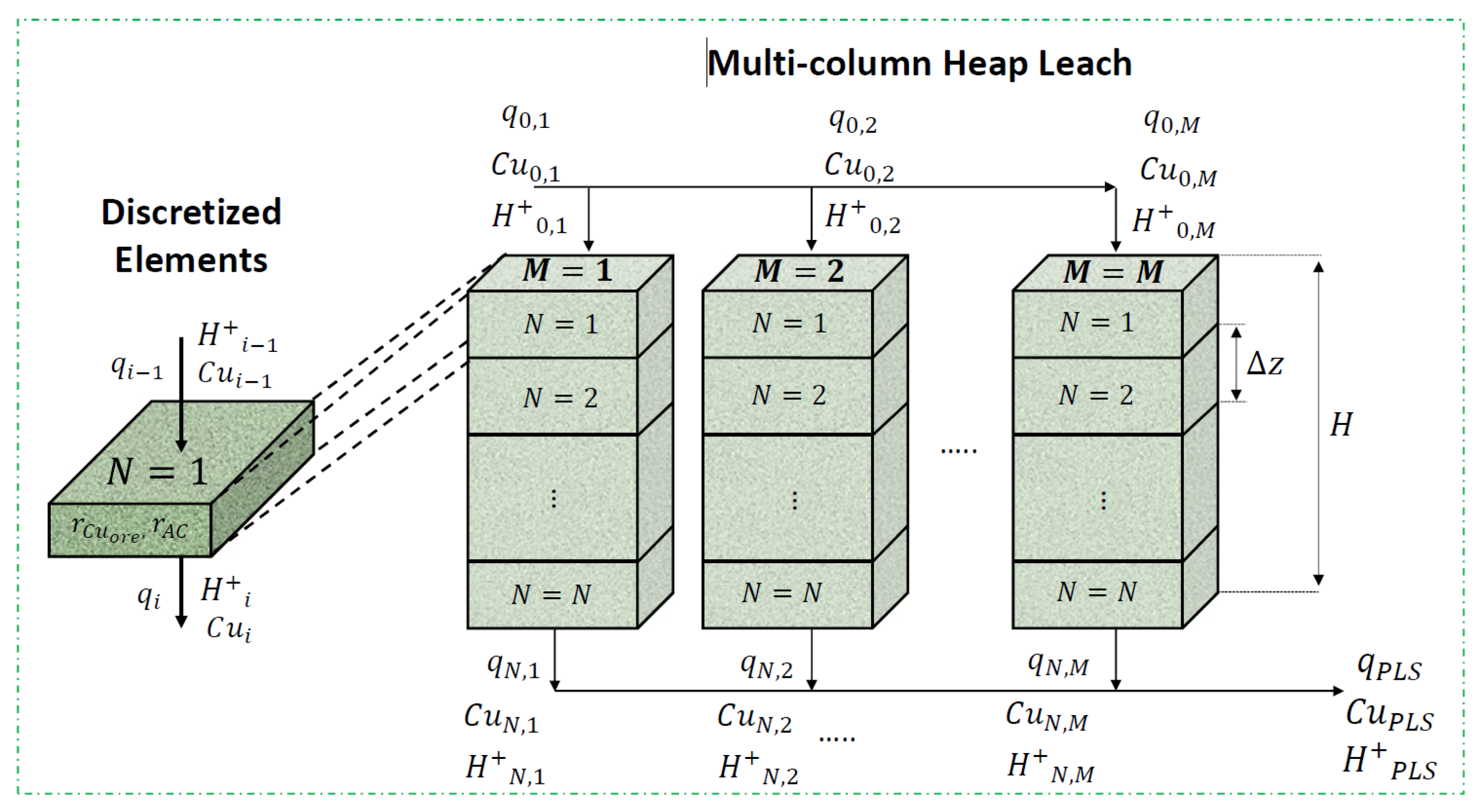
  • Dominant vertical axis: Mass balances are primarily considered in the vertical direction, assuming negligible lateral flow [24].
  • Hydraulic relationships for unsaturated flow media: The model incorporates explicit dependencies on drainage and dynamic moisture, representing the solution content per mineral portion.
  • Neglect of diffusional mass flux: The diffusional mass flux is disregarded due to its significantly lower magnitude than advective mass fluxes, in line with Assumption 2.
These simplifications allow for a more manageable and focused modeling approach while still capturing the essential aspects of the heap leaching process, since the lateral and even vertical effects of diffusion and convection are not particularly significant at the macroscale but only in the study of the microscale. The mass balance equations of the heap leaching module are described by the following ordinary differential equations (ODEs) [1,21,22]:
d θ i d t = q i q i 1 ,
d C u i d t = 1 z q i C u i q i 1 C u i 1 + r C u   i × 1 θ i C u i d θ i d t ,
d C u o r e , i d t = r C u o r e ,   i ,
d H i + d t = 1 z q i H i + q i 1 H i 1 + + r H i + b r C u   i × 1 θ i H i + d θ i d t ,
d A C i d t = r A C i ,
where θ , C u , C u o r e , H + , and A C are the moisture content percentages in the leaching solution, the aqueous copper concentration, the copper ore, the acid concentration, and the acid consumption, respectively. q i and q i 1 represent the outflow and inflow, respectively. r C u   i , r H i + , r C u o r e ,   i , and r A C i represent the specific reaction rates. Parameter b is a stoichiometric coefficient that relates to the amount of acid consumed per amount of dissolved copper in the ore.
Figure 1 illustrates a discretized schematic of the heap leaching module [25]. The model incorporates essential phenomena, including advective mass flow, storage accumulation, and chemical reactions for mineral generation or consumption. The vertical axis of the module was discretized using N elements, each representing a volume unit in the system, and integrated in time to represent each i = 1,2 , , N volume, where N is the number of elements, and z is the discrete element length equal to H / N . Discretization allows for integrating the module’s behavior over time, capturing the dynamics of each volume element.
An upwind numerical scheme estimates the flow and concentration at the interfaces between adjacent discretized elements, ensuring an accurate representation of the mass transport. This approach treats the system as a series of vertically stacked stages, each corresponding to a discrete volume element [26]. The concentration within the volume element determines the output concentration flow. Also, the output low module q i is the input flow q i 1 of the subsequent module.
Since a vertical flow with no lateral flow is assumed, and the model can have multiple M columns, where each column has multiple N modules, the size of the process model is defined by the multiplied N × M .
The initial conditions x 0 R 5 N M × 1 of the discretized ODE model are calculated as [15]
x 0 = θ i , 0 C u i , 0 C u o r e , i , 0 H i , 0 + A C i , 0 = θ i n i 0 g C u m M C u 0 C u m a x m ,
where θ i n i is the initial moisture content, g C u represents the copper grade (copper law), m is the mineral mass pile section, M C u is the molecular weight of the mineral, and C u m a x is the maximum acid consumption in each module volume.
The mineral mass pile section m is calculated as follows:
m = V p ρ a p ,
where ρ a p is the bulk density ore, and V p is the stack section volume in [ m 3 ] calculated as the width times the length times the height between the number of elements N :
V p = W · L · H / N .

2.1. Kinetic Reactions

The kinetics of the heap leaching process involve the dissolution of copper and other components, influenced by the reagents’ reaction and/or transport kinetics and involved constituents, mainly by the diffusion controlling stage [23,27]. This paper employs a model to describe the kinetic equations, assuming that the copper oxide ore’s copper grade and the degree of mineral liberation do not affect the leaching rate. Additionally, it is assumed that the concentration of the reactants remains constant throughout the leaching process.
The reaction rate equations initially in this work relied on min–max Functions (9)–(11), which are known to be non-differentiable for all time points. To facilitate the application of observers that rely on linearization, it is proposed to replace the min–max functions with exponential functions, which are smooth and differentiable. These exponential functions, as described by Hashemzadeh et al. [19] in Equations (12) and (13), provide a suitable alternative for the modeling of the system dynamics and enable the effective implementation of the state observers.
The min–max reaction rates r C u   i , r H i + , r C u o r e ,   i , and r A C i are defined as
r C u o r e , i = C u o r e , i , 0 K τ C u o r e × min max 1 2 C u o r e , i C u o r e , i , 0 C u o r e , i , 0 + 1 + 1 1 / 3 2 , 0 , 150 ,
r A C i = r H i + = A C i , 0 K τ A C , H + × min max 1 2 A C i A C i , 0 A C i , 0 + 1 1 / 3 2 , 0 , 150 ,
r C u i = r C u o r e , i M C u m p ,
The value of 150 used in the min–max Equations (9) and (10) is a numerical technique to prevent unrealistic behavior for the reaction rate (e.g., taking the value of +infinity at time zero ( t = 0 )).
The redefined exponential reaction rates r ~ C u o r e , i       , r ~ H i +     ,   a n d r ~ A C i     are defined in the following equations (the equation for r C u i (11) does not need redefinition):
r ~ C u o r e , i     = C u o r e , i , 0 K τ C u o r e C u o r e , i C u o r e , i , 0 C u o r e , i , 0 + 1 φ 1 ,
r ~ H i +     = r ~ A C i     = A C i , 0 K τ H + , A C A C i A C i , 0 A C i , 0 + 1 φ 2 ,
with acid consumption and a copper kinetic time constant:
K τ H + , A C = H i + m H + , A C 1 C m a x 1 K A C 2 R q H + , A C ,
K τ C u o r e 1 = H i + m C u 1 g C u 1 K C u 1 2 R q C u ,
K τ C u o r e 2 = 1 g C u 1 0.5 K C u 2 2 R q C u ,
σ τ C u S = 1 1 + e H i + 5 0.1 ,
K τ C u o r e = K τ C u o r e 1 1 σ τ C u o r e + K τ C u o r e 2 σ τ C u o r e ,
where φ 1 is the topological exponent for copper, m C u   a n d q C u are the copper reaction orders, φ 2 is the topological exponent for acid consumption, with m H + , A C , and q H + , A C the acid consumption reaction orders. Both φ 1 and φ 2 vary between 0 and 1 [19].
The topological parameters used in this work were found using the particle swarm optimization (PSO) algorithm [28]. The PSO method finds the optimal set of Φ = φ 1 , m C u , q C u , φ 2 , m H + , A C , q H + , A C ; Φ ϵ 0 , 4 by minimizing an optimization problem. The expression for the optimization problem in finding the absolute mean square error (MSE) for the min–max reactions equations presented in (9) and (10) compared to the exponential reactions’ equations defined in (12) and (13). The following equation calculates the optimization problem:
ϕ C u o r e = ϕ 1 = 1 n i = 1 n x i , C u o r e x ~ i , C u o r e 2 ω C u o r e , ϕ A C = ϕ 2 = 1 n i = 1 n x i , A C x ~ i , A C 2 ω A C , Φ = a r g m i n ϕ C u o r e + ϕ A C ,
where x i is the value of the min–max model, x ~ i is the value of the Hazhemzadeh model, n is the number of samples, ω C u o r e = 2000 , and ω A C = 4000 are weight parameters for the estimated state.

2.2. Hydrodynamic Relationship

Hydrodynamics is crucial in efficiently extracting valuable minerals or metals from the leach pad. Factors such as permeability, particle size distribution, compaction, leaching rate, flow distribution, and control influence hydrodynamic behavior. The equations below describe hydrodynamic behavior in the porous media. They allow optimal irrigation for a heap, that is, the leaching solution that should be used to irrigate the modules available on the surface.
The flow q is calculated using Darcy’s velocity vector expression:
q = k r , w k μ w g r a d p w ρ w g ,
where μ w is the dynamic viscosity of the fluid, k is the permeability of the medium, k r , w corresponds to the relative permeability of the medium, p w is the density of the fluid phase, and g is the gravity vector.
The most used models for permeability in unsaturated soils are the Brooks–Corey and Van Genuchten models, with the choice depending on the specific shape of the retention curve [29]. This paper uses the Brooks–Corey unsaturated equations due to their simpler mathematical formulation and fewer parameters, which facilitate analytical solutions. Previous work that has successfully applied the Brooks–Corey model under similar conditions supports this choice [30].
Therefore, the unsaturated permeability is [31]
k r , w = S e 2 + 3 n ,
where n is a characteristic parameter of the medium, which is constant and comes from experimentation, and S e is the effective saturation:
S e = θ i e r e s e sat e r e s ,
where e r e s = ϕ S r , w corresponds to the residual saturation of the liquid, where ϕ and S r , w are the porosity of the residual saturation of the liquid, respectively, and e s a t = ϕ 1 S r , n corresponds to the saturation of the liquid, where S r , n is the residual saturation of the gas.
The term g r a d p w is calculated as
g r a d p w   =   p c i + 1     p c i Δ z ,
The magnitude of the capillary pressure p c is defined as
p c = p e S e 1 / n ,
where p e is a characteristic parameter of the medium equal to n . Normally, n is a parameter related to the distribution of the pores inside the solid, and p e is a parameter related to the conditions for a continuous network of flow channels to exist within the medium. The hydrodynamic parameters listed in Table 1 were obtained considering a silt-loam soil, based on the work of [32].

3. State Observer Design

Heap leaching allows us to measure variables from both the liquid and solid phases. In the liquid phase, we can track key components like dissolved acid ( H + ) and copper ( C u ) concentrations in the pregnant leach solution (PLS). Typically, the acid concentration can be measured offline on a small scale (in a laboratory) using an automatic titrator. In contrast, the aqueous copper concentration can be calculated online through atomic absorption methods on small and large scales (in mining processes). These measurements provide valuable information for assessing the chemical composition and dynamics of the leaching process, which is sampled in shifts during the day for laboratory testing [3].
While liquid measurements are straightforward, the solid phase presents significant challenges. We can potentially measure factors like copper in the ore, the concentration of other materials (gangue or acid consumption), moisture content, and granulometry, among others. However, obtaining these measurements in a column of crushed material within the heap leaching process is complex. The voluminous and compact structure of the heap makes it challenging to access and intervene to obtain representative measurements. Additionally, modifying the compaction of the heap can lead to potential landslides, further hindering the acquisition of accurate and representative measurements in the solid stage of heap leaching. Compaction increases moisture retention, increasing the risk of landslides [4].
Given these challenges, we focus on measurable liquid phase variables: acid ( H + ) and copper ( C u ) concentrations. These offer valuable real-time information through online monitoring. Solid phase variables like copper in the ore ( C u o r e ), acid consumption ( A C ), and the moisture content ( θ ) are more difficult to measure directly, and therefore, they are estimated.
This work employs two estimation techniques: an Extended Kalman Filter (EKF) [10] and the Unscented Kalman Filter (UKF) [11] for the estimation of copper in the ore ( C u o r e ), acid consumption ( A C ), and moisture content ( θ ) states (1,3,5) based on acid ( H + ) and copper ( C u ) measurements (2–4). Figure 2 illustrates the block diagram of the proposed state observers for the heap leaching process. It consists of two key stages:
  • Prediction Stage (green area): A process model, incorporating uncertainties, predicts the system’s future state based on its current state.
  • Update Stage (yellow area): The predicted state and the measurement error are combined using the Kalman gain ( K ). This updates the system’s estimated state (represented by x ^ ) and the error covariance matrix ( P ).
This two-step process helps the observers continuously refine their estimate of the system’s state as new measurements become available.
Assumption 1: 
The EKF formulation is continuous–discrete due to discrete concentration measurements [33,34].
Assumption 2: 
The EKF assumes that the system’s dynamics can be linearized locally using the Jacobian.
Assumption 3: 
Both filters assume that the process and measurement noise are Gaussian noise.
Assumption 4: 
The inlet/outlet flow rate ( q i 1 , q i ) is considered a known input to the process.
Assumption 1 is appropriate for the heap leaching process, as concentrations such as aqueous copper and acid are measured discretely over time. Consequently, it provides continuous estimates based on these measurements. In contrast, Assumption 2 is only valid for the EKF, as the UKF (a more advanced variant of the EKF) incorporates the concept of sigma points to capture the uncertainty distribution without requiring linearization. The main difference is that the EKF linearizes the system model at each step to perform calculations. In contrast, the UKF utilizes a strategic set of sigma points to represent the probability distribution of the system’s state. This approach allows UKF to manage nonlinearities more effectively and often results in better filtering performance, especially for higher-order systems like ours.
For the design, we have a discretized process model with uncertainties, which was obtained using the Euler method ( t m = 0.5 days) by discretizing the continuous model Equations (1), (3), and (5) represented in the nonlinear state transition function f x ^ k , u k . The choice of a fraction of a day for t m ensures seeing possible dynamic responses, especially associated with irrigation and flow through the porous medium and mineral kinetics.
The discretized model of the process is
x ^ k = x ^ k 1 + t m f x ^ k 1 , u k 1 + w k 1 ,
where x ^ k   ϵ   R 3 N M × 1 is the state vector, and w k 1   ϵ   R 3 N M × 1 0 , Q j , k 1 with j = E K F , U K F is the state process white noise. The discrete measurements vector z k   ϵ   R 2 N M × 1 is the discrete measurement given by
z k = h x ^ k + υ k ,
where the nonlinear measurement function h x ^ k corresponds to the solution of the discretized Equations (2) and (4), and υ k   ϵ   R 2 N M × 1 is the measurement white noise sequence of the zero mean and variance R k   ( υ k   ( 0 , R _ { j , k } ) with j = E K F , U K F .
Finally, the discretized estimated state variables, inputs ( u k 1 ), and outputs for the EKF and UKF are
x ^ k 1 = θ   C u o r e   A C T ϵ   R 3 N M × 1 u k 1 = q 0   C u , 0   H 0 + ϵ   R 3 M × 1 h x ^ k = C u   H + T ϵ   R 2 N M × 1 ,
where q 0 ,   C u , 0 , and H 0 + are the input flow, copper in irrigation (raffinate), and the initial acid concentration, respectively. The C u , 0 takes values below 0.1 g/L; therefore, in this work, we assume it to be equal to zero. Appendix A and Appendix B show the EKF and UKF equations and variable definitions, respectively.

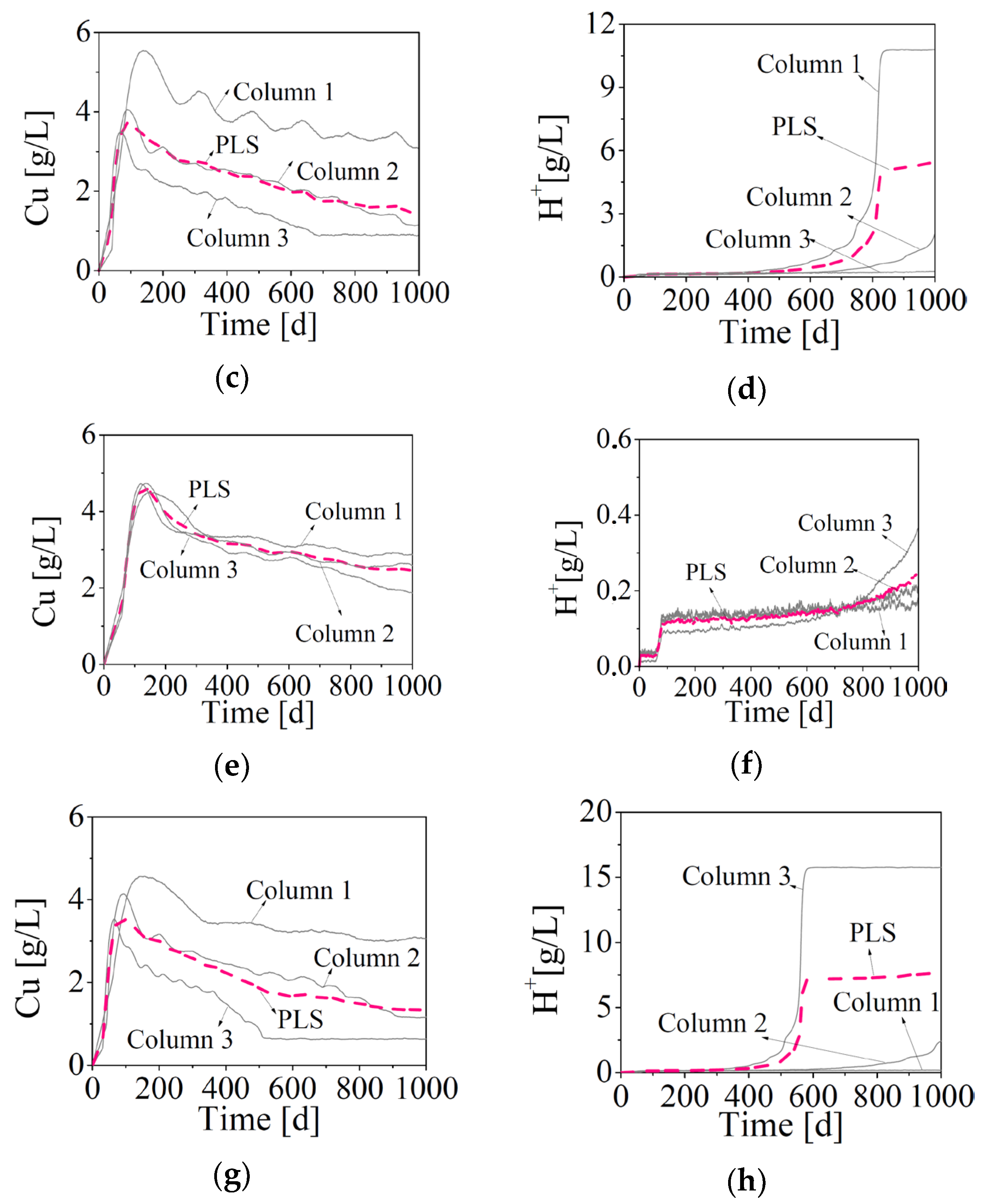
3.1. Measurements Multicolumn Model

The discrete measurements vector z k (26) is assigned in different ways, depending on the number of columns to be analyzed in the heap leaching (Figure 1). When considering a single column ( M = 1 Figure 1), the size of the model state depends on the total number of differential equations multiplied by the number of discretized elements in the heap N , resulting in 5 N . In this case, the pregnant leach solution (PLS) is obtained from the last volume of the heap. The output in this stage corresponds to the immediate concentration of the variable:
z k = C u N , 1 k H N , 1 k + 2 N M ,   1 + υ C u , k υ H + , k 2 N M ,   1 .
In a more realistic scenario—specifically, with multiple 1D columns without lateral flows arranged in parallel form ( M = 1 : M ), as shown in Figure 1—the PLS output is calculated as the average of the measurable concentrations from the last levels of each column, multiplied by the input flow of each column ( q N , M ), and divided by the average individual input flow for each column. This approach considers the contributions from multiple columns to obtain the PLS concentration, resulting in the following expression:
z k = i M C u N , i k q N , i k i M q N , i k i M H N , i k + q N , i k i M q N , i k 2 N M ,   1 + υ C u , k υ H + , k 2 N M ,   1 .

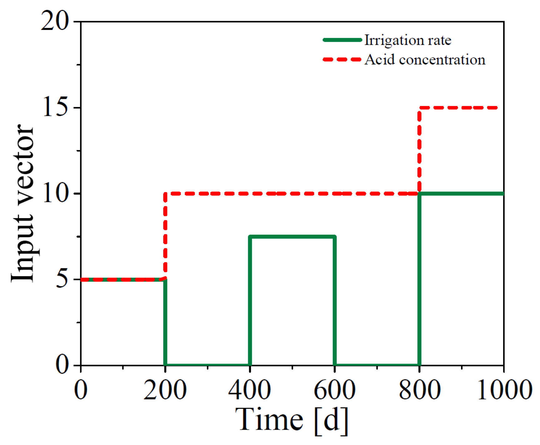
3.2. Simulation Cases

Four scenarios were designed to test the observers’ robustness. These scenarios assume different conditions in the leaching columns to demonstrate their ability to simulate industrial-scale situations while considering various operational aspects. The irrigation conditions, acid concentration, and copper grade are modified in each scenario to assess the observer’s versatility before significant changes in the critical model parameters.
Each scenario consists of one or three 1D columns, and each permanent column contains ten ( N = 10 ) discretized levels (irrigation levels). The four scenarios are described as follows:
The first simulated scenario involves one column ( M = 1 ) and ten elements ( N = 10 ), totaling 50 differential equations. This column spans an expansive area of 7500 m 2 . The flow within the column is strictly vertical, devoid of any lateral movement. The heap is irrigated from the top ( N = 1 ), with the liquid descending element by element until it reaches the final element ( N = 10 ), from which the leached sample is extracted.
The second, third, and fourth simulated scenarios involve multiple heap leach columns ( M = 3 ), each comprising 10 volumes ( N = 10 ). Together, these scenarios encompass a substantial area of 22,500 m 2 . Each scenario is simulated under distinct operating conditions. The flow behavior within these scenarios mirrors that of the first scenario, with the measurement being the total PLS of the combined output (effluents) from the three columns (Equation (29)). To obtain accurate results, 150 differential equations are solved per observer. Detailed parameter values of each scenario can be found in Table 1. Notably, the copper grade is determined on-site by the miners themselves.
To ease the readability of the result, we replace the use of the input flow q with the operational variable in the metallurgy field called the irrigation rate T r v , which is the flow per surface irrigated expressed in L / h m 2 :
T r v , j = q o , j · 1000 24 .

4. Results, Analysis, and Discussion

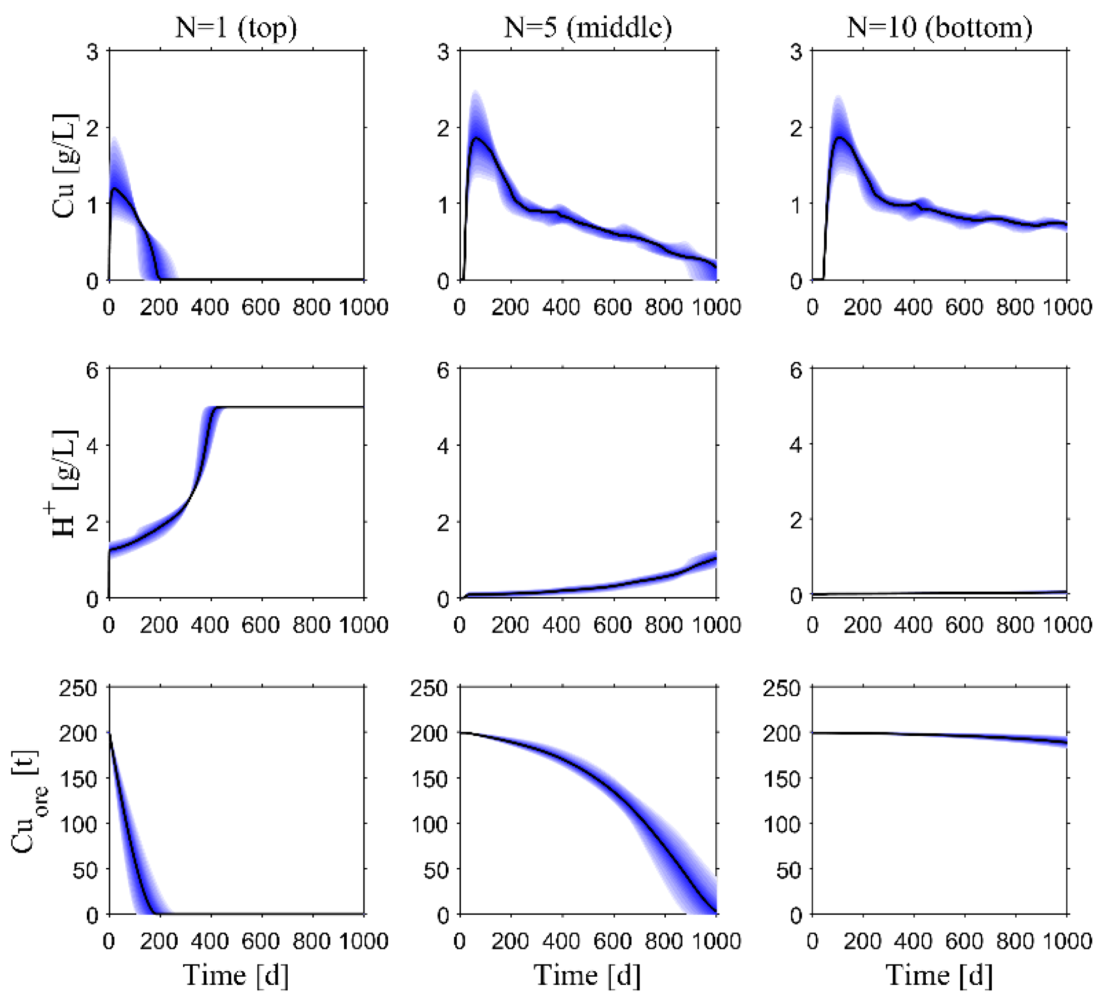
4.1. Preliminary Simulation of the Heap Leaching Model

For simulating the 1D heap leaching model, the MATLAB @2024a (ODE15s) environment was utilized. The model parameters (Equations (1)–(5)) were obtained experimentally and are presented in Table 2. The model’s initial conditions are calculated using Equation (6). The simulation duration is 1000 days (approximately 2.7 years). The concentration profiles of C u , H + , and C u o r e are illustrated in Figure 3 for the 1D heap leach with one column ( M = 1 ) and ten elements ( N = 10 ). A sensitivity simulation was conducted to determine how the principal profiles of the model respond to variations in the key parameters. To illustrate the simulation, the kinetic model parameters ( K C u 1 , K C u 2 ,   a n d   K A C ) were randomly drawn from a uniform distribution for 1000 simulations, with the irrigation rate fixed at T r v = 7.5   L / h m 2  and  H 0 + = 5   g / L .
Figure 3 illustrates the natural behavior of the leaching process model under parametric variability. The black curve in the center of the blue shading represents the average trend. At N = 1 (upper module), aqueous copper ( C u ) shows a rapid increase as it leaches with the highest acid concentration ( H + ). Conversely, the copper in the ore ( C u o r e ) exhibits a rapid decrease. At N = 5 , copper leaching slows down due to the significantly lower acid availability than in the first stage. Finally, the copper concentration is much more sustained at the bottom level ( N = 10 ). This is because it represents the cumulative copper leached to the end (PLS). The acid concentration is practically zero, as it has been depleted in this scenario. Copper in the ore remains high, indicating that more time (or higher acid concentration) is needed for complete leaching.
Regarding responses under 50% parameter variability, the size of the blue shading indicates each variable’s sensitivity. We observe that aqueous copper demonstrates the highest sensitivity, with its concentration able to change by up to 1 g/L based on parameter variations. Copper in the ore exhibits cumulative sensitivity, meaning its response accumulates over time. Lastly, the acid concentration shows moderate sensitivity relative to the other variables.

4.2. Observers’ Results

To enhance the robustness of the observers, the initial conditions of the estimated states, x ^ 0 , E K F and x ^ 0 , U K F , were randomly set by sampling from a normal distribution, with the mean the nominal value of the model initial conditions and a standard deviation of 0.1. The initial values of the covariance matrices P 0 , E K F and P 0 , U K F were chosen to match the observer’s initial conditions [33], given adequate knowledge of the model’s initial conditions. For the UKF observer, the values of the sigma point tuning parameters are α = 1 × 10 3 , β = 2 , and κ = 0 . As mentioned above, the EKF and UKF equations and variable definitions for the EKF and UKF are provided in Appendix A and Appendix B.
To select the corresponding values of the noise covariance matrices linked to the process and the measurement, several datasheets for copper quantifiers and acid meters used in the mining industry were analyzed. The most common method for measuring sulfuric acid in the PLS within a plant laboratory is the typical titration method. In [36], the standard deviation varied from 0.001 to 0.1. For the copper measurement, a reference value was obtained from the datasheet [37]. The final sigma values employed for C u and H + were σ C u 2 = σ H + 2 = 10 3 . These values presume a low sampling variability, as measurements are taken in duplicate at the minimum to minimize outliers, mainly due to sensor variability. Subsequently, the covariance matrix of the measurement noise is constructed as
R E K F , t k + 1 , R U K F , t k + 1   =   d i a g σ C u 2 , σ H + 2 .
The covariance matrix of the process noise is
Q E K F , t k + 1 , Q U K F , t k + 1 = σ Q 2 I 3 N M × 3 N M ,
where σ Q = 10 4 and I 3 N M × 3 N M are the identity matrix. In theory, Q can take values of zero, since the process variance is neglected; however, this restricts the model’s ability to learn exclusively from the measurements without considering the process model. Q values can be derived, for instance, through a Monte Carlo simulation while assessing the expected variability in the input variables. Nonetheless, for this study, we approximate by using typical values for the relative variance, which is about 1%.

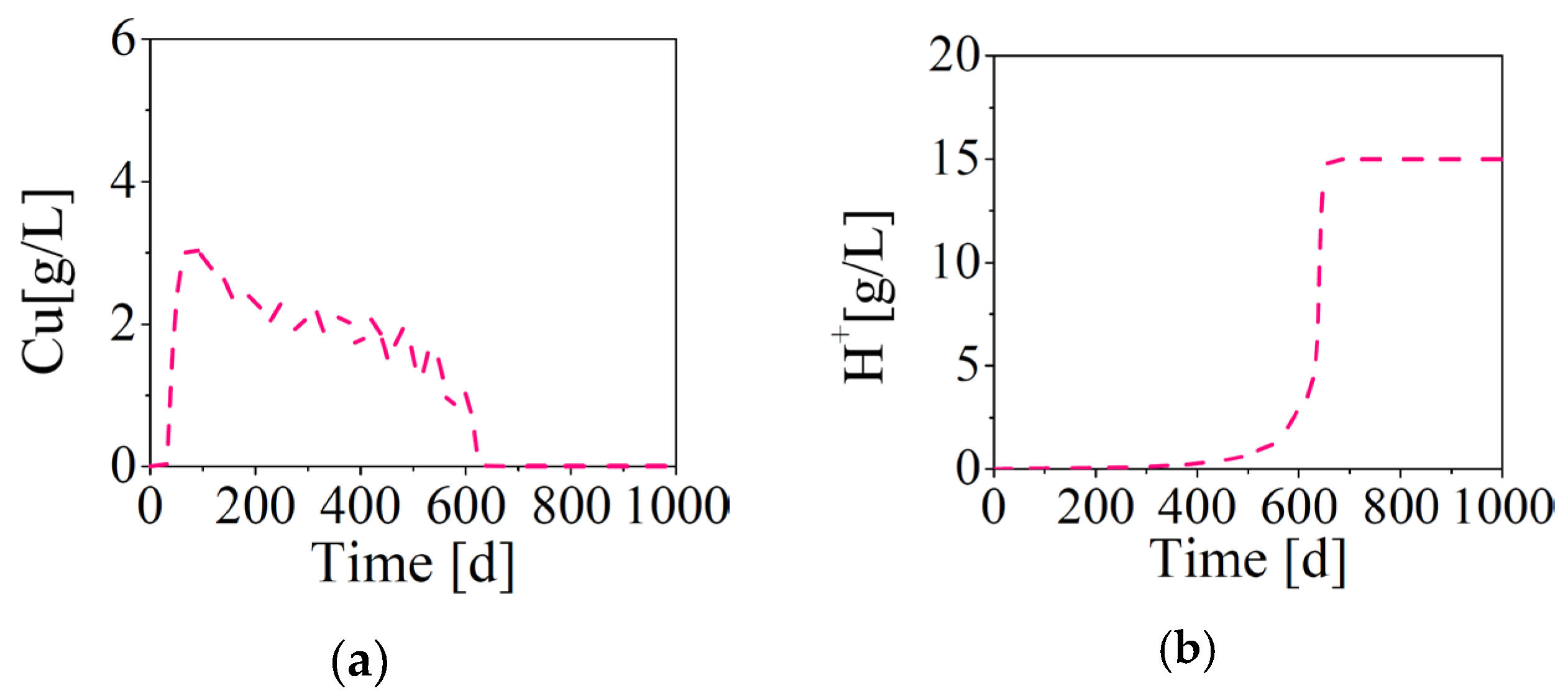
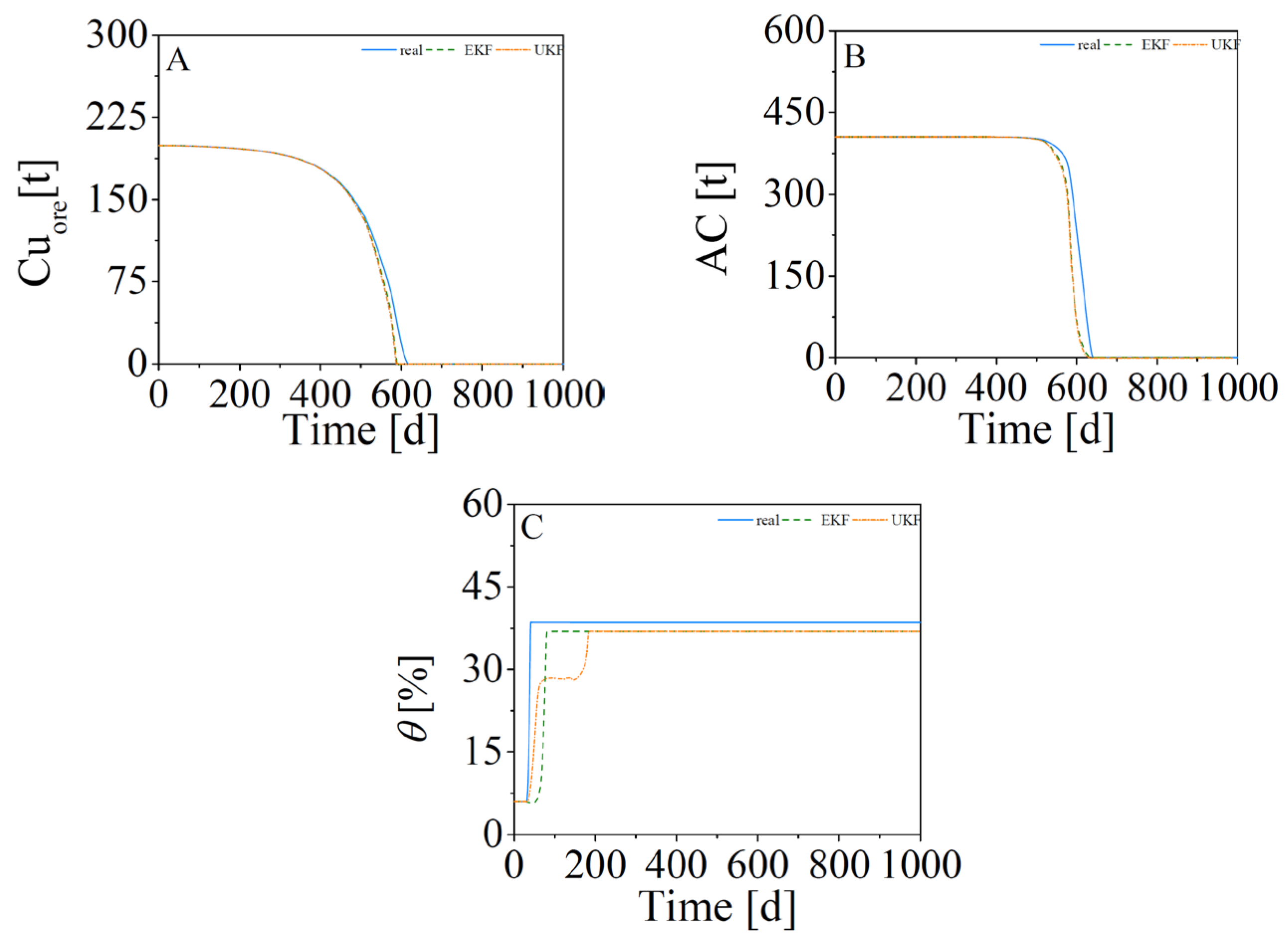
4.3. Simulation of One Module (Scenario 1)

As previously stated, each scenario will be simulated under different conditions to replicate real-world situations involving intermittent irrigation supply interruptions. For instance, in a scenario where the irrigation rate or acid concentration varies, the values utilized are outlined in Table 1. Following the procedure defined by Equation (33), various values for T r v and H o + are applied over a specified time interval ( t ). The initial acid concentration is adjusted at different time intervals, while the irrigation rate functions in an on/off mode, alternating between watering and pausing for specific durations. The T r v and H o + used for Scenarios 1 and 4 are depicted in Figure 4.
i ,   T r v ,   H o + = 1 , 5,7.5,10 , 5,10,15 i f   t < 200 2,0 , 5,10,15 i f   200 < t < 400 2 , 5,7.5,10 , 5,10,15 2,0 , 5,10,15 3 , 5,7.5,10 , 5,10,15 i f   400 < t < 600 i f   600 < t < 800 i f   t > 800
Figure 5a shows the measurement variables for the first scenario for copper dynamics, and Figure 5b shows the measurement variables for acid dynamics. By analyzing these curves, we see that, as acid irrigation increases within the column, the aqueous copper content rises before eventually being completely leached out. To establish a ground truth for the estimations of the state observers, the ‘actual’ values of the estimated variables are derived from the mathematical model of the heap leaching process.
Figure 6 illustrates the estimations of the state observers. We can see that both observers achieve satisfactory asymptotic convergence of the estimations. Figure 6A presents the estimate at the final stage ( N = 10 ) for the concentration of copper remaining in the ore. Figure 6B displays the estimates for acid consumption, while Figure 6C reveals the estimates for the moisture content within the leaching heap.
When comparing the performance of the observers shown in Figure 6A–C, it becomes evident that the estimation error remains relatively small, even in the presence of noisy measurements. However, the Unscented Kalman Filter (UKF) displays some irregular behavior on day 200 in response to sudden changes in the values of T r v and H o + (see Figure 5), as demonstrated by the moisture content curves. The abrupt change in the input variables results in the saturation of the modulus, leading to fluctuations in the performance of the UKF filter.

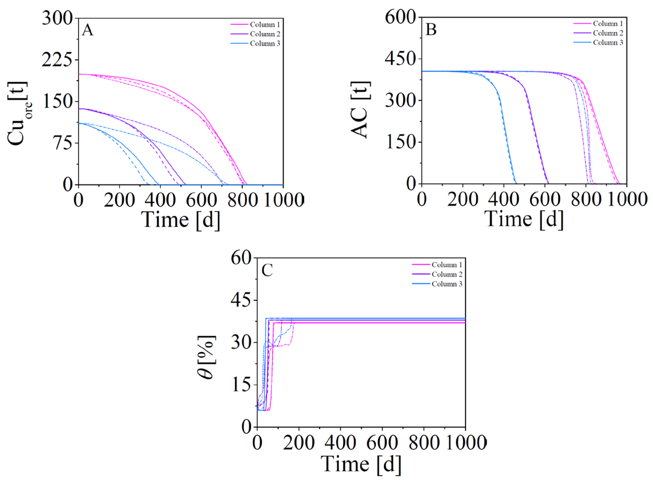
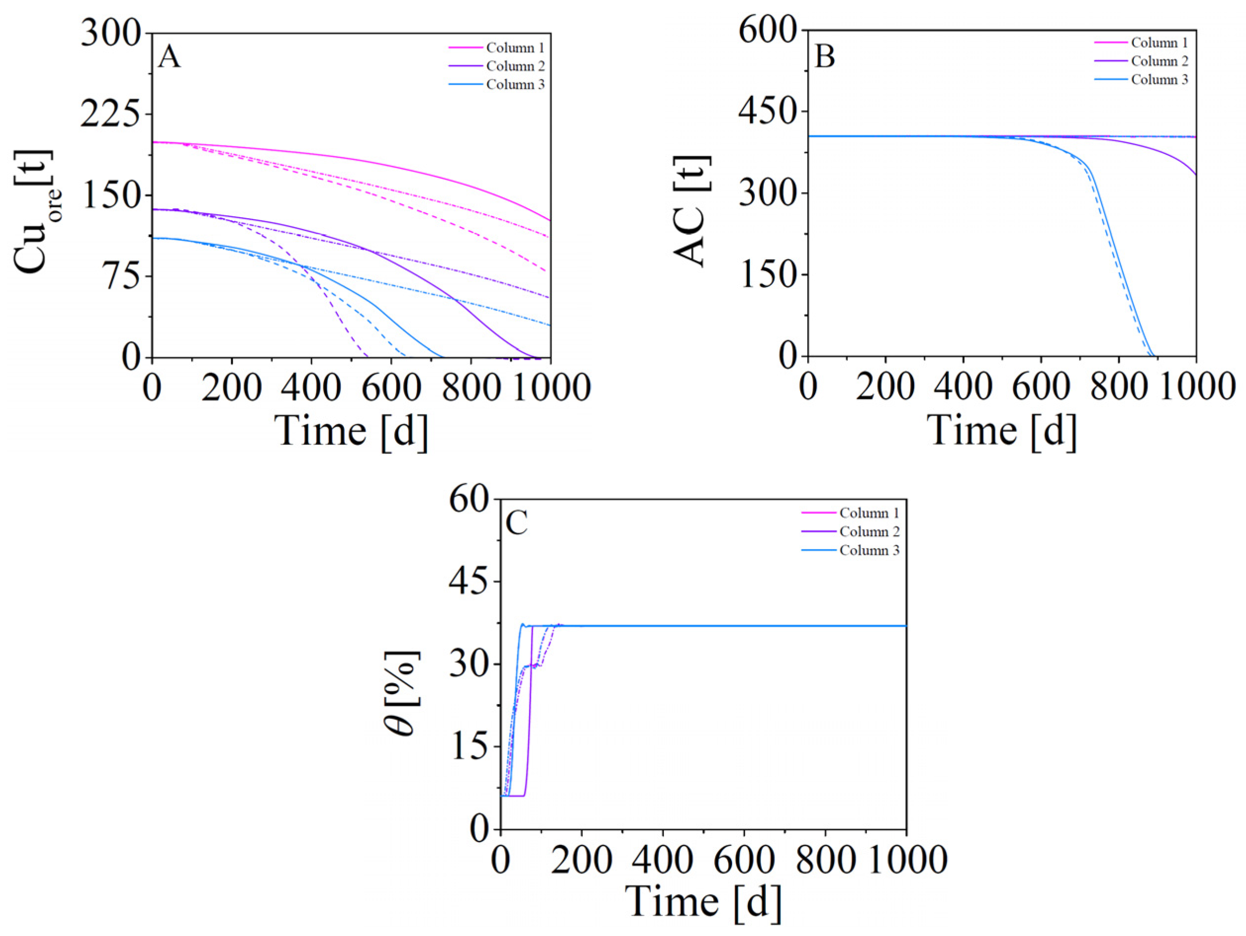
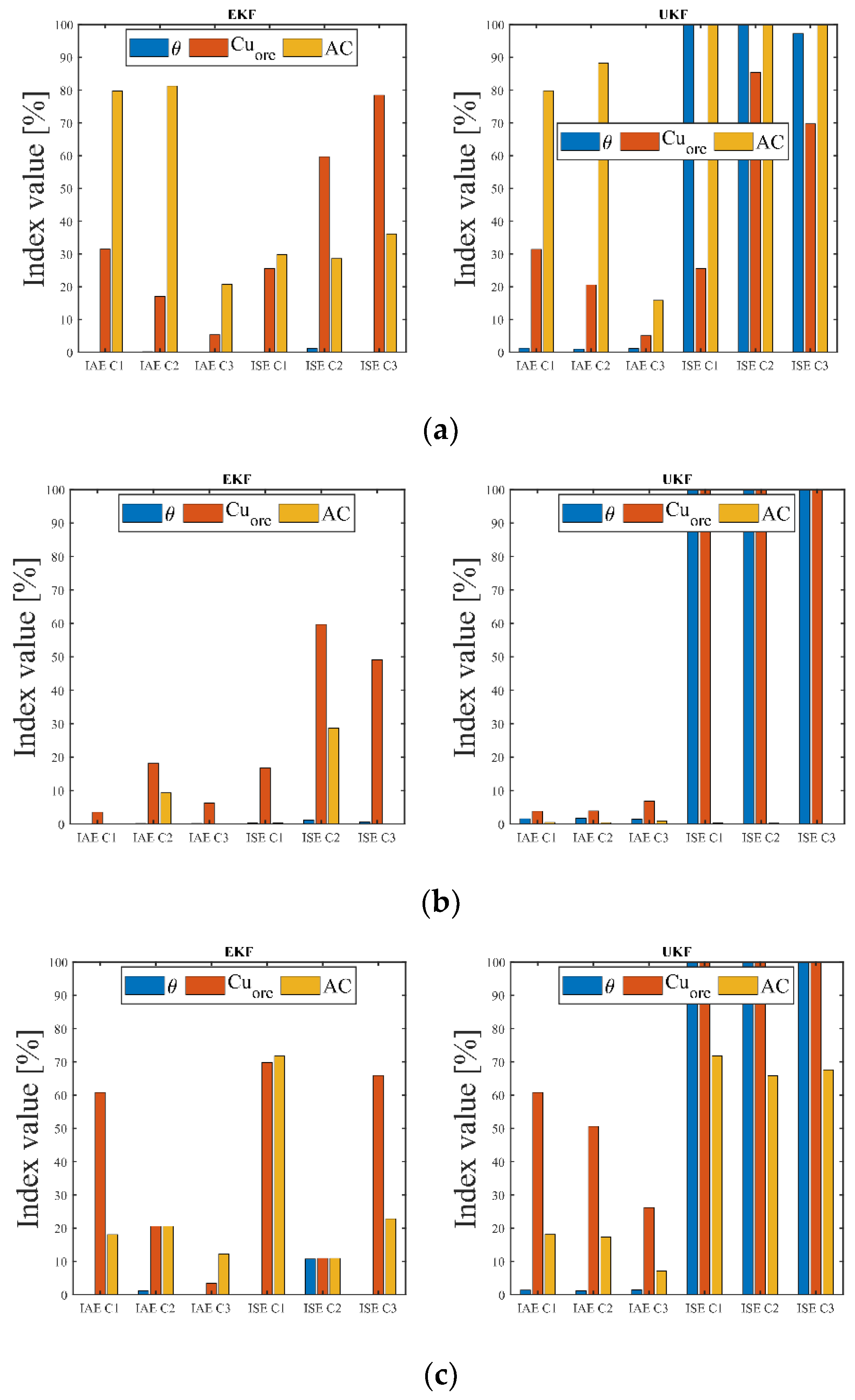
4.4. Simulation of Multiple Modules (Scenario 2–4)

The observers undergo a more realistic test scenario where they are evaluated for estimating multiple columns. This scenario is deemed more realistic than the one modeled in Scenario 1. The goal is to assess the observers’ robustness under various critical characteristics in each column. These characteristics include parameters such as copper grade, differing irrigation rates, and initial acid concentrations in each column. By introducing such diverse and challenging conditions, the evaluation seeks to thoroughly investigate the observers’ performance and reliability in practical scenarios.
The measurement variables for Scenario 2 are shown in Figure 5c,d, those for Scenario 3 in Figure 5e,f, and the measurements for Scenario 4 are presented in Figure 5g,h. In cases with multiple columns, the actual measurement is the PLS (dashed pink lines) derived from the combined output of the M columns, representing an average across them. This average is illustrated by the dashed pink line in the figures mentioned above.
Figure 7A–C present the estimations of the state observers for Scenario 2. A clear trend has developed concerning the impact of irrigation rates on the leaching process. In Column 3, leaching occurs significantly faster when a higher irrigation rate ( T r v = 10 ) is applied. In contrast, in Column 1, with a lower irrigation rate ( T r v = 5 ), the leaching process advances slower.
It is important to note that, despite these variations, the Extended Kalman Filter (EKF) consistently provides satisfactory estimations. However, the Unscented Kalman Filter (UKF) faces challenges in achieving an asymptotic estimate. Notably, UKF’s error increases as the leaching process speeds up, indicating that the transformation based on sigma points may not be optimal for the stages characterized by rapid leaching. This observation raises questions about the appropriateness of the sigma point transformation in accurately capturing the system dynamics during these fast leaching phases.
The results shown in Figure 8 for Scenario 3 illustrate a contrasting scenario: the irrigation rate is kept constant, while the acid concentration in each column varies. Notably, a low irrigation rate leads to a slower overall process. Furthermore, an initial increase in acid concentration does not guarantee a complete recovery of copper, as evidenced by the presence of copper in the column’s mineral at the end of the simulation.
In this scenario, the observers initially align with the real values. However, divergence from the true values becomes noticeable after approximately 200 days. The convergence thereafter becomes slower, indicating that stability and convergence are more successfully achieved when the persistent excitation originates from a variable such as the irrigation rate rather than from changes in the acid concentration. This insight suggests that a consistent and variable irrigation rate contributes more favorably to the stability and convergence of the observers in this context.
Scenario 4, shown in Figure 9, represents a combination of the previously discussed scenarios. In this case, the irrigation rate varies for all three columns, exhibiting an on/off behavior. The first column, with a lower initial acid concentration ( H o + = 5   g / L ), undergoes the slowest leaching process. Consequently, both filters provide highly accurate estimates of the actual values.
However, the leaching process accelerates significantly as the initial acid concentration ( H o + ) increases. At this point, the observers, particularly UKF, diverge from their ideal values. In Scenario 4, the UKF shows a notable overshoot in the estimated moisture response (Figure 9C). These observations highlight the observers’ sensitivity to variations in the leaching process. As the process intensifies, maintaining the accuracy of the estimates becomes more challenging, leading to divergences and, in the case of the UKF, a slight overshooting in the estimated moisture response.
The recovery of copper is the most critical indicator of the leaching process. When the concentration of copper in the ore, C u o r e , approaches zero over time, it signifies the successful leaching of all copper from the ore. Accurately estimating the C u o r e can provide insights into the expected monthly copper recovery. The results obtained, as shown in Figure 6A, Figure 7A, Figure 8A, and Figure 9A, illustrate how the actual values and their estimates tend toward zero at differing intervals. The speed at which the C u o r e converges depends on the reaction rate. In contrast, the speed at which observers approach the real value is contingent upon the parametric adjustment for each observer.
To compare both observers under equal conditions, their respective initial values of the covariance matrices, measurement noise, and processes are set to be the same. The only difference lies in the internal mechanism of each observer to solve and construct the final observation equation (Equation (A9) for the EKF and Equation (A28) for the UKF). Figure 10a–c present bar charts indicating the values in percentages of the performance indices: Integral Absolute value Error (IAE) and Integral Squared Error (ISE) calculated for the moisture content, C u o r e , and acid consumption in Scenarios 2, 3, and 4 for each column. A visual analysis reveals that the EKF consistently exhibits lower values than the UKF, with occasional instances where the UKF exceeds 100%. EKF demonstrates superior performance in the estimations, followed by the UKF. Scenario 2 yields the lowest values of the IAE and ISE indices for all the estimated variables. The results of the IAE and ISE indices are also displayed in Table 3.
The application of EKF and UKF to the leaching process is highly valuable. The EKF/UKF algorithms effectively estimate the state variables of interest. In a real-time monitoring environment, they can provide up-to-the-minute estimates of the state variables, enabling continuous monitoring of the leaching process and timely adjustments of the control parameters as needed. This can enhance the process efficiency and product quality. Conversely, all estimated state variables can be utilized in feedback control schemes [30] to adapt the leaching process to changing conditions, such as variations in the ore composition or feedstock properties. Future work includes the laboratory-scale experimentation of a multi-column leaching system using EKF/UKF for state estimations to validate the PLS profiling approach and refine the measurement functions.

5. Conclusions

This study investigates the application of nonlinear Bayesian observers (EKF and UKF) in the context of heap leaching, a highly complex nonlinear process. The unique physical structure of heap leaching presents significant challenges in obtaining accurate measurements. In this work, aqueous phase measurements, including copper and acid concentrations, were utilized to estimate the state variables of the solid phase, namely the concentrations of copper in the ore and acid consumption. Additionally, the moisture content of the heap was estimated. Realistic simulations of heap leaching were implemented to develop the process model, and experiments using this simulated model were conducted. Discrete versions were derived based on the simulated model, tailored explicitly for the proposed nonlinear observers. These observers were then tested across various scenarios designed to challenge the structure of critical variables within the system. Significantly, the observers achieved commendable accuracy, with the EKF registering an Integral Absolute Error (IAE) of only 0.041% and an Integral Square Error (ISE) of 0.069% for the moisture content in Scenario 2. In Scenario 4, the IAE for the EKF was as low as 0.044% for the moisture content and 18.04% for acid consumption, demonstrating high fidelity in these complex scenarios. To provide a quantitative perspective, across the challenging conditions in Scenario 2, the EKF outperformed the UKF with lower performance indices, notably achieving an IAE that was 12 times lower for the moisture content and an ISE that was 182 times lower for the copper concentration estimation in Column 1. Similarly, in Scenario 4, which introduced variable irrigation rates, the EKF showed superior control over the estimation errors, with a 96.5% lower IAE in moisture content estimation compared to the UKF for Column 1. These precise quantitative metrics highlight the robustness of the nonlinear Bayesian observers, particularly the EKF, in accurately tracking state variables under dynamically changing conditions within the heap leaching process. Although these results are based on high-fidelity simulations, future works will focus on validating the proposed methods using actual heap leaching production data in collaboration with industrial partners to confirm their applicability under real-world conditions. An open question for future research is how values diverging from those recommended in the UKF’s design parameters ( α , β , and κ ) would affect the performance differences between the Extended Kalman Filter (EKF) and the Unscented Kalman Filter (UKF).

Author Contributions

L.B.-M. and S.D.-Q.; methodology, L.B.-M.; software, L.B.-M. and S.D.-Q.; validation, L.B.-M. and S.D.-Q.; investigation, L.B.-M.; resources, J.R.-d.-S. and H.E.; data curation, L.B.-M. and S.D.-Q.; writing—original draft preparation, L.B.-M. and S.D.-Q.; writing—review and editing, L.B.-M., S.D.-Q., J.R.-d.-S. and H.E.; supervision, J.R.-d.-S. and H.E.; project administration, J.R.-d.-S. and H.E.; funding acquisition, J.R.-d.-S. and H.E. All authors have read and agreed to the published version of the manuscript.

Funding

This research was funded by the National Research and Development Agency (ANID) of Chile through project grant AFB230001 for the Advanced Mining Technology Center (AMTC), and the Cost center No: 02030402-999, Department of Electricity, Universidad Tecnológica Metropolitana.

Data Availability Statement

The data presented in this study are available on request from the corresponding author due to (The data are property of the mining companies).

Conflicts of Interest

The authors declare no conflicts of interest. The funders had no role in designing this study, collecting data, analyzing the results, interpreting the findings, writing this manuscript, or deciding to publish its results.

Abbreviations

The following abbreviations are used in this manuscript:
Greek Letters
z Discrete element length
θ Moisture content [%]
Superscripts
^ Estimated
Variables
r ~ C u o r e Smooth Copper in the ore rate [kg/h]
r ~ H + Smooth Acid reaction rate [kg/h]
A C Acid consumption concentration [t]
C u Aqueous copper concentration [g/L]
C u o r e Copper concentration in the ore [t]
E K F Extended Kalman Filter
H Heap Height [m]
H + Acid concentration [g/L]
L Heap Length [m]
M Number of columns
m Mineral mass pile section [kg/m]
M C u Molecular weight of the mineral [kg/kmol]
N Number of elements
q i 1 Inlet flow [ m 3 /h]
q i Outlet flow [ m 3 /h]
r A C Acid consumption rate [kg/h]
r C u o r e Copper in the ore rate [kg/h]
r C u Copper reaction rate [kg/h]
r H + Acid reaction rate [kg/h]
T r v Irrigation rate [L/h- m 2 ]
U K F Unscented Kalman Filter
V p Heap Volume [ m 3 ]
W Heap Width [m]

Appendix A. The Extended Kalman Filter (EKF)

This work uses a continuous–discrete version of the EKF [29,30]. This type of formulation is suitable for the heap leaching process, since concentrations such as aqueous copper and acid are discretely measured over time. Therefore, in the continuous–discrete EKF formulation, continuous estimates are made based on discrete–time measurements.
This section presents the equations corresponding to the various stages of the EKF. The EKF operates recursively, continually refining its estimate based on incoming measurements. It comprises two main stages: the prediction stage and the update stage. To simplify the observer equations presented in this paper, it is assumed that all elements of the estimated state, the covariance matrix, and the Kalman gain have the appropriate dimensions.
First, the initialization of the states and covariance ( k = 0 ) is defined as
x ^ 0 , E K F = E x 0 + r a n d 0.1 ,
P 0 , E K F = d i a g x ^ 0 , E K F .
Prediction Stage
Step 1. State prediction
x ^ k k 1 = f ( x ^ k 1 k 1 , u k 1 ) ,
where x ^ k k 1 ϵ   R 3 N M × 1 .
Step 2. Covariance prediction  P ^
P ^ k k 1 = A k x ^ k P k 1 k 1 A k x ^ k T + Q E K F , k 1 ,
with P ^ k k 1 ϵ R 3 N M × 3 N M , and Q E K F , k 1 is the covariance matrix of state process noises. The Jacobian, denoted as A k , is the derivative of f with respect to x ^ k 1 k 1 , evaluated at point k 1 k 1 , and is derived through the following partial derivatives:
A k x ^ k = f x x ^ k 1 k 1 , u k 1 ,
with A k   ϵ   R 3 N M × 3 N M .
Step 3. Measurement prediction
z ^ k k 1 = h x ^ k k 1 .
The Jacobian, denoted as C k , is the derivative of h with respect to x ^ k k 1 , evaluated at point k k 1 . It is assessed at the predicted state before the measurement update and is derived through partial derivatives, expressed as
C k = h x x ^ k k 1 ,
with C k   ϵ   R 2 N M × 3 .
Update Stage
Step 4. Kalman gain calculation  K k
K k = P ^ k k 1 C k T ( C k   P ^ k k 1 C k T + R E K F , k ) 1 ,
where K k   ϵ   R 3 N M × 2 , and R E K F , k is the covariance matrix of the measurement errors.
Step 5. State estimation and covariance update
x ^ k k = x ^ k k 1 + K k ( z k z ^ k k 1 ) ,
P ^ k k = P ^ k k 1 K k C k P ^ k k 1 .

Appendix B

A general framework for the recursive estimation of the UKF is presented in the following stages. The initialization of the states and covariance ( k = 0 ) is defined as
x ^ 0 , U K F = x ^ 0 , E K F ,
P 0 , U K F = P 0 , E K F .
Prediction Stage
Step 1. Selection of sigma points
The mean x ^ k 1 k 1 and variance P ^ k 1 k 1 of each state x k 1 k 1 are approximated by the sigma points selected ( k   ϵ   1 , , ):
X ^ 0 , k 1 k 1 = x ^ k 1 k 1 ,   i = 0 ,
X ^ x , k 1 k 1 = x ^ k 1 k 1   + ( n + λ ) P ^ k 1 k 1 i , i = 1 , . . . , L ,
X ^ v , k 1 k 1 = x ^ k 1 k 1   n + λ P ^ k 1 k 1 i , i = L + 1 , . . . , 2 L ,
where L is the length of the estimated state x ^ k 1 k 1 . The scaling parameter λ = α 2 L + κ L depends on the constant α , which determines the spread of the sigma points around x ^ k 1 k 1   and is usually set to 1 × 10 4 α 1 , and the constant κ is usually set to 0. ( n + λ ) P ^ k 1 k 1 i is the i t h column of the matrix square root of ( n + λ ) P ^ k 1 k 1 .
Finally, the sigma points are regrouped in the following matrix of L rows and 2 L + 1 columns:
K k = P ^ k k 1 C k T ( C k   P ^ k k 1 C k T + R E K F , k ) 1 ,
where X ^ x , k 1 k 1 are the sigma point rows associated with the state and parameters, and X ^ v , k 1 k 1 is the sigma point rows associated with the state and parameter process noises.
Step 2. State prediction
Each sigma point is propagated through the process model to yield a set of transformed samples.
X ^ i , k k 1 = f X ^ i , k 1 k 1 , u k 1 ,   i = 0,1 , , 2 L ,
The predicted mean is computed as
x ^ k k 1 = i = 1 2 L W i m X ^ i , k k 1 .
Step 3. Covariance prediction
P ^ k k 1 = i = 1 2 L W i c X ^ i , k k 1 x ^ k k 1 X ^ i , k k 1 x ^ k k 1 T + Q U K F , k 1 ,
with
W i c = W i m = 1 2 L + λ ,   i = 1 , 2 L ,
W 0 c = λ L + λ + 1 α 2 + β ,   i = 0
W 0 m = λ L + λ ,   i = 0
where β is used to incorporate prior knowledge of the state’s distribution and is set to the optimal value of β = 2 .
Step 4. Measurement prediction
z i , k k 1 = h x ^ i , k k 1 ,   i = 0,1 , , 2 L ,
z ^ i , k k 1 = i = 0 2 L W i m z i , k k 1 .
Update Stage
In this stage, as in the EKF, the Kalman matrix is calculated, and the estimated state and the covariance matrix are updated using the state increased with the sigma points. The vector of the measurements is also a function of the sigma points.
Step 5. Kalman gain calculation
P z k , z k = i = 0 2 L W i c z i , k k 1 z ^ i , k k 1 × z i , k k 1 z ^ i , k k 1 T + R U K F , k ,
P x k , z k = i = 0 2 L W i c X ^ i , k k 1 x ^ k k 1 × z i , k k 1 z ^ i , k k 1 T ,
K k = P x k , z k P z k , z k 1 .
Step 6. State estimation and covariance update
x ^ k k = x ^ k k 1 + K k z k z ^ i , k k 1 ,
P ^ k k = P ^ k k 1 K k P z k , z k K k T .

References

  1. Petersen, J. Heap leaching as a key technology for recovery of values from low-grade ores—A brief overview. Hydrometallurgy 2016, 165, 206–212. [Google Scholar] [CrossRef]
  2. Ghorbani, Y.; Franzidis, J.-P.; Petersen, J. Heap leaching technology—Current state; innovations; future directions: A review. Miner. Process. Extr. Metall. Rev. 2016, 37, 73–119. [Google Scholar] [CrossRef]
  3. Estay, H.; Lois-Morales, P.; Montes-Atenas, G.; del Ruiz del Solar, J.R. On the Challenges of Applying Machine Learning in Mineral Processing and Extractive Metallurgy. Minerals 2023, 13, 788. [Google Scholar] [CrossRef]
  4. Daud, O.; Correa, M.; Estay, H.; del Solar, J.R.-D. Monitoring and Controlling Saturation Zones in Heap Leach Piles Using Thermal Analysis. Minerals 2021, 11, 115. [Google Scholar] [CrossRef]
  5. Tang, M.; Esmaeili, K. Heap Leach Pad Surface Moisture Monitoring Using Drone-Based Aerial Images and Convolutional Neural Networks: A Case Study at the El Gallo Mine, Mexico. Remote Sens. 2021, 13, 1420. [Google Scholar] [CrossRef]
  6. He, J.; DuPlessis, L.; Barton, I. Heap leach pad mapping with drone-based hyperspectral remote sensing at the safford copper mine, arizona. Hydrometallurgy 2022, 211, 105872. [Google Scholar] [CrossRef]
  7. Herrera, L.; Jun, K.J.; Baker, J.; Agrawal, B.N. Deep Learning Based Object Attitude Estimation for a Laser Beam Control Research Testbed. Appl. Artif. Intell. 2023, 37, 2151191. [Google Scholar] [CrossRef]
  8. Herrera, N.; Sinche Gonzalez, M.; Okkonen, J.; Canales, R.M. Predicting Flowability at Disposal of Spent Heap Leach by Applying Artificial Neural Networks Based on Operational Variables. Minerals 2023, 14, 40. [Google Scholar] [CrossRef]
  9. Thenepalli, T.; Chilakala, R.; Habte, L.; Tuan, L.Q.; Kim, C.S. A brief note on the heap leaching technologies for the recovery of valuable metals. Sustainability 2019, 11, 3347. [Google Scholar] [CrossRef]
  10. Kalman, R.E. A New Approach to Linear Filtering and Prediction Problems. J. Basic Eng. 1960, 82, 35–45. [Google Scholar] [CrossRef]
  11. Julier, S.; Uhlmann, J. Unscented filtering and nonlinear estimation. Proc. IEEE 2004, 92, 401–422. [Google Scholar] [CrossRef]
  12. Xu, W.; Zhang, F. FAST-LIO: A Fast, Robust LiDAR-Inertial Odometry Package by Tightly-Coupled Iterated Kalman Filter. IEEE Robot. Autom. Lett. 2021, 6, 3317–3324. [Google Scholar] [CrossRef]
  13. Xu, W.; Cai, Y.; He, D.; Lin, J.; Zhang, F. FAST-LIO2: Fast Direct LiDAR-Inertial Odometry. IEEE Trans. Robot. 2022, 38, 2053–2073. [Google Scholar] [CrossRef]
  14. Wang, Y.; Wen, X.; Gu, B.; Gao, F. Power Scheduling Optimization Method of Wind-Hydrogen Integrated Energy System Based on the Improved AUKF Algorithm. Mathematics 2022, 10, 4207. [Google Scholar] [CrossRef]
  15. Bucci, A.; Franchi, M.; Ridolfi, A.; Secciani, N.; Allotta, B. Evaluation of UKF-Based Fusion Strategies for Autonomous Underwater Vehicles Multisensor Navigation. IEEE J. Ocean. Eng. 2023, 48, 1–26. [Google Scholar] [CrossRef]
  16. Garcia, R.; Pardal, P.; Kuga, H.; Zanardi, M. Nonlinear filtering for sequential spacecraft attitude estimation with real data: Cubature Kalman Filter, Unscented Kalman Filter and Extended Kalman Filter. Adv. Space Res. 2019, 63, 1038–1050. [Google Scholar] [CrossRef]
  17. Kaur, H.; Sahambi, J. Vehicle Tracking in Video using Fractional Feedback Kalman Filter. IEEE Trans. Comput. Imaging 2016, 4, 550–561. [Google Scholar] [CrossRef]
  18. Sotiropoulos, F.; Asada, H. Autonomous Excavation of Rocks Using a Gaussian Process Model and Unscented Kalman Filter. IEEE Robot. Autom. Lett. 2020, 5, 2491–2497. [Google Scholar] [CrossRef]
  19. Hashemzadeh, M.; Dixon, D.G.; Liu, W. Modelling the kinetics of chalcocite leaching in acidified cupric chloride media under fully controlled pH and potential. Hydrometallurgy 2019, 189, 105114. [Google Scholar] [CrossRef]
  20. Cariaga, E.; Martínez, R.; Sepúlveda, M. Estimation of hydraulic parameters under unsaturated flow conditions in heap leaching. Math. Comput. Simul. 2015, 109, 20–31. [Google Scholar] [CrossRef]
  21. McBride, D.; Gebhardt, J.E.; Croft, T.N.; Cross, M. Modeling the hydrodynamics of heap leaching in sub-zero temperatures. Miner. Eng. 2016, 90, 77–88. [Google Scholar] [CrossRef]
  22. Vargas, T.; Estay, H.; Arancibia, E.; Díaz-Quezada, S. In situ recovery of copper sulfide ores: Alternative process schemes for bioleaching application. Hydrometallurgy 2020, 196, 105442. [Google Scholar] [CrossRef]
  23. Saldaña, M.; Gálvez, E.; Robles, P.; Castillo, J.; Toro, N. Copper Mineral Leaching Mathematical Models—A Review. Materials 2022, 15, 1757. [Google Scholar] [CrossRef]
  24. Ghasemzadeh, H.; Sanaye Pasand, M.; Mollanouri Shamsi, M. Experimental study of sulfuric acid effects on hydro-mechanical properties of oxide copper heap soils. Miner. Eng. 2018, 117, 100–107. [Google Scholar] [CrossRef]
  25. Estay, H.; Díaz-Quezada, S. Deconstructing the Leaching Ratio. Min. Metall. Explor. 2020, 37, 1329–1337. [Google Scholar] [CrossRef]
  26. Evans, L.C. Partial Differential Equations; American Mathematical Society: Providence, RI, USA, 2022; Volume 19. [Google Scholar]
  27. Wadsworth, M.; Yong Sohn, H. Rate Processes of Extractive Metallurgy; Springer: Boston, MA, USA, 1979. [Google Scholar] [CrossRef]
  28. Kennedy, J.; Eberhart, R. Particle swarm optimization. In Proceedings of the ICNN’95—International Conference on Neural Networks, Perth, WA, Australia, 27 November–1 December 1995; Volume 4, pp. 1942–1948. [Google Scholar] [CrossRef]
  29. Robertson, S.; Basson, P.; van Staden, P.; Petersen, J. Properties governing flow of solution and air through crushed ore for heap leaching: Part ii unsaturated dual-phase flow. Hydrometallurgy 2023, 215, 105990. [Google Scholar] [CrossRef]
  30. Canales, C.; Díaz-Quezada, S.; Leiva, F.; Estay, H.; del Solar, J.R. Control of heap leach piles using deep reinforcement learning. Miner. Eng. 2024, 212, 108707. [Google Scholar] [CrossRef]
  31. Brooks, R.H.; Corey, A. Hydraulic Properties of Porous Media; Hydrology Papers; Colorado State University: Fort Collins, CO, USA, 1964. [Google Scholar]
  32. Dingman, S.L. Physical Hydrology; Waveland Press: Long Grove, IL, USA, 2015. [Google Scholar]
  33. Bárzaga-Martell, L.; Duarte-Mermoud, M.A.; Ibáñez-Espinel, F.; Gamboa-Labbe, B.; Saa, P.A.; Pérez-Correa, J.R. A robust hybrid observer for monitoring high-cell density cultures exhibiting overflow metabolism. J. Process Control 2021, 104, 112–125. [Google Scholar] [CrossRef]
  34. Bogaerts, P.; Wouwer, A. Parameter identification for state estimation—Application to bioprocess software sensors. Chem. Eng. Sci. 2004, 59, 2465–2476. [Google Scholar] [CrossRef]
  35. Herrar, U. Influencia de las Concentraciones de Ácido Sobre la Cinética de Lixiviación de un Mineral Oxidado de Cobre. Bachelor’s Thesis, Universidad de Chile, Santiago, Chile, 2001. [Google Scholar]
  36. Kahlert, H.; Meyer, G.; Albrecht, A. Colour maps of acid–base titrations with colour indicators: How to choose the appropriate indicator and how to estimate the systematic titration errors. ChemTexts 2016, 2, 7. [Google Scholar] [CrossRef]
  37. Spectroscopy Editors. Copper Quantification in Geological Samples by Flame AAS. Spectroscopy. November 2023. Available online: https://www.spectroscopyonline.com/view/copper-quantification-geological-samples-flame-aas (accessed on 22 April 2025).
Figure 1. Multi-columns heap leaching diagram and flow through a discretized element.
Minerals 15 00521 g001
Figure 2. Block diagram of the state observer for the heap leaching process.
Minerals 15 00521 g002
Figure 3. Results of the sensitivity simulations. Profiles of copper C u , acid H + , and copper in the ore C u o r e at different column heights: top (N = 1), middle (N = 5), and bottom (N = 10).
Minerals 15 00521 g003
Figure 4. Variable behavior for the initial acid concentration and irrigation rate input vector. Irrigation rate T r v (green) and initial acid concentration H o + (red).
Minerals 15 00521 g004
Figure 5. Scenario 1: Copper ( C u ) (a) and acid ( H + ) (b). Scenario 2: Copper ( C u ) (c) and acid ( H + ) (d). Scenario 3: Copper ( C u ) (e) and acid ( H + ) (f). Scenario 4: Copper ( C u ) (g) and acid ( H + ) (h). All measurements were taken from Columns 1, 2, and 3 (Grey), with PLS (dashed pink).
Minerals 15 00521 g005aMinerals 15 00521 g005b
Figure 6. Scenario 1: Estimate of copper in the ore, acid consumption, and moisture content for a column of the heap leaching. (A) Copper in the ore ( C u o r e ); (B) acid consumption ( A C ); (C) moisture content ( θ ). Mathematical model value (sky blue), EKF (dashed green), and UKF (short dashed-dot orange).
Minerals 15 00521 g006
Figure 7. Scenario 2: Estimate of copper in the ore, acid consumption, and moisture content for a column of the heap leaching. (A) Copper in the ore ( C u o r e ); (B) acid consumption ( A C ); (C) moisture content ( θ ). Column 1: Mathematical model value (magenta), EKF (dash magenta), and UKF (short dash dot magenta); Column 2: Mathematical model value (violet), EKF (dash violet), and UKF (short dash dot violet); Column 3: Mathematical model value (sky blue), EKF (dash sky blue), and UKF (short dash dot sky blue).
Minerals 15 00521 g007
Figure 8. Scenario 3: Estimate of copper in the ore, acid consumption, and moisture content for a column of the heap leaching. (A) Copper in the ore ( C u o r e ); (B) acid consumption ( A C ); (C) moisture content ( θ ). Column 1: Mathematical model value (magenta), EKF (dash magenta), and UKF (short dash dot magenta); Column 2: Mathematical model value (violet), EKF (dash violet), and UKF (short dash dot violet); Column 3: Mathematical model value (sky blue), EKF (dash sky blue), and UKF (short dash dot sky blue).
Minerals 15 00521 g008
Figure 9. Scenario 4: Estimate of copper in the ore, acid consumption, and moisture content for a column of the heap leaching. (A) Copper in the ore ( C u o r e ); (B) acid consumption ( A C ); (C) moisture content ( θ ). Column 1: Mathematical model value (magenta), EKF (dash magenta), and UKF (short dash dot magenta); Column 2: Mathematical model value (violet), EKF (dash violet), and UKF (short dash dot violet); Column 3: Mathematical model value (sky blue), EKF (dash sky blue), and UKF (short dash dot sky blue).
Minerals 15 00521 g009
Figure 10. Performance indices for representative multi-column scenarios. (a) Scenario 2. (b) Scenario 3. (c) Scenario 4.
Minerals 15 00521 g010
Table 1. Values of irrigation rates, acid concentration, and copper grade (copper law) for each scenario and column.
ScenarioColumn
Index “j”
Copper
Grade
Irrigation Rates
T r v , j L / h m 2
Acid. Conc.
H 0 + g / L
110.5110[5;7.5;10][5;10;15]
210.5110510
20.35087.510
30.28331010
310.511055
20.350857.5
30.2833510
410.5110[5;7.5;10][5;10;15]
20.3508[5;7.5;10][5;10;15]
30.2833[5;7.5;10][5;10;15]
Table 2. Parameters for heap leaching.
ParameterDescriptionValueUnitsRef.
R Granulometry1 c m [This work]
b Stoichiometric coefficient of acid to copper1.54 g / g [35]
ρ a p Bulk density ore1.8 t / m 3 [35]
W Heap Module Width50 m [This work]
L Heap Module Length50 m [This work]
H Heap Module Height50 m [This work]
ρ s o l Solution density1 t / m 3 [35]
θ i n i Initial moisture content6 % [This work]
C u m a x Maximum acid consumption ineach module volume30 k g / t [35]
K C u 1 Copper kinetic constant 1502.5110 d a y g / c m 2 L [35]
K C u 2 Copper kinetic constant 287.7702 d a y / c m 2 [35]
K A C Acid consumption kinetic constant1.15 × 103 d a y g / c m 2 L [35]
φ 1 Copper topological exponent0.4492--[This work]
φ 2 Acid consumption topological ex-ponent0.9983--[This work]
m C u Copper reaction order1.2722--[This work]
q C u Copper reaction order1.5238--[This work]
m H + , A C Acid consumption reaction order3.2658--[This work]
q H + , A C Acid consumption reaction order0.5171--[This work]
e r , w Residual saturation of the liquid0.115 c m 3 / c m 3 [32]
e r , n Residual saturation of the gas0.148 c m 3 / c m 3 [32]
k Permeability of the medium7.34 × 1013 m 2 [32]
ϕ Porosity0.485 c m 3 / c m 3 [32]
p e Characteristic parameter of the medium7710 P a [32]
n Characteristic parameter of the medium0.19--[28]
Table 3. Results of the performance indices for scenarios 1–4 for EKF and UKF.
Var.Scenario 2Scenario 3Scenario 4Scenario 1
EKFUKFEKFUKFEKFUKFEKFUKF
IAE C1 θ 0.0411.2500.0891.5700.0441.3402.6903.070
C u o r e 31.4431.403.5743.48060.8260.801.5901.960
A C 79.7079.800.05049.4018.0418.107.5208.340
IAE C2 θ 0.1911.0000.1921.5701.2031.120----
C u o r e 17.0920.6018.093.86020.5720.60----
A C 81.2888.3090.3040.9020.5717.30----
IAE C3 θ 0.0171.1000.2001.4500.0501.470----
C u o r e 5.3415.0606.2086.8903.4132.260----
A C 20.7815.800.079945.012.077.130----
ISE C1 θ 0.06912.6035.6015.800.05913.5036.1025.30
C u o r e 25.2925.5016.7019.3069.7769.7029.4039.30
A C 29.8429.9035.70339.071.7471.8087.7096.20
ISE C2 θ 1.20310.701.20018.2010.7412.10----
C u o r e 59.7485.4059.7018.2010.9410.90----
A C 28.6631.1028.70242.010.9465.80----
ISE C3 θ 0.0099.72060.7015.100.08016.60----
C u o r e 78.4769.7049.1059.7065.9040.30----
A C 36.1421.10104.2129.022.9567.60----
Disclaimer/Publisher’s Note: The statements, opinions and data contained in all publications are solely those of the individual author(s) and contributor(s) and not of MDPI and/or the editor(s). MDPI and/or the editor(s) disclaim responsibility for any injury to people or property resulting from any ideas, methods, instructions or products referred to in the content.

