
Dynamic Error Bat Algorithm: Theory and Application to Magnetotelluric Inversion
 ,
,
Abstract
1. Introduction
2. Materials and Methods
2.1. Magnetotelluric Sounding Method
2.2. BA Principle
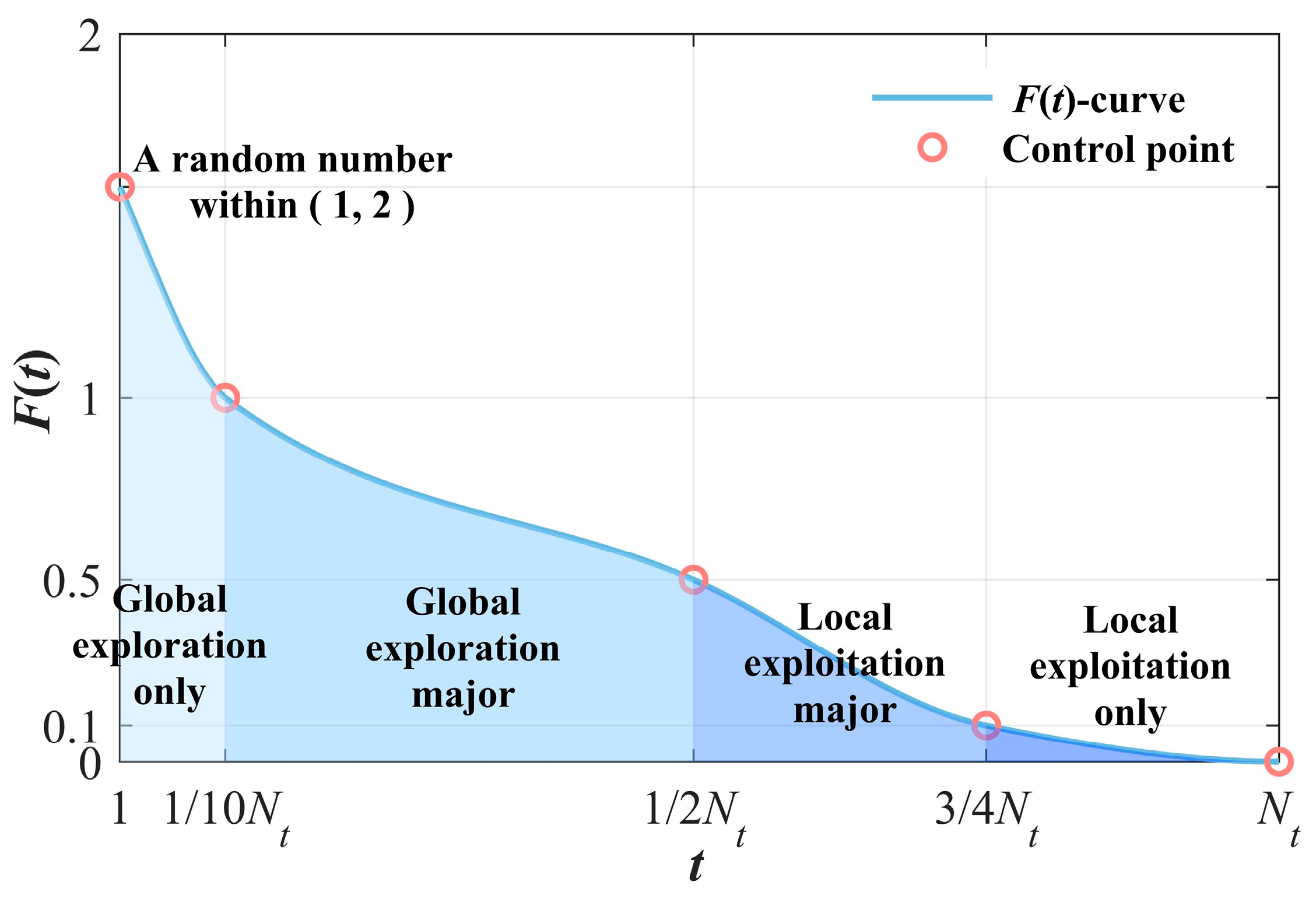
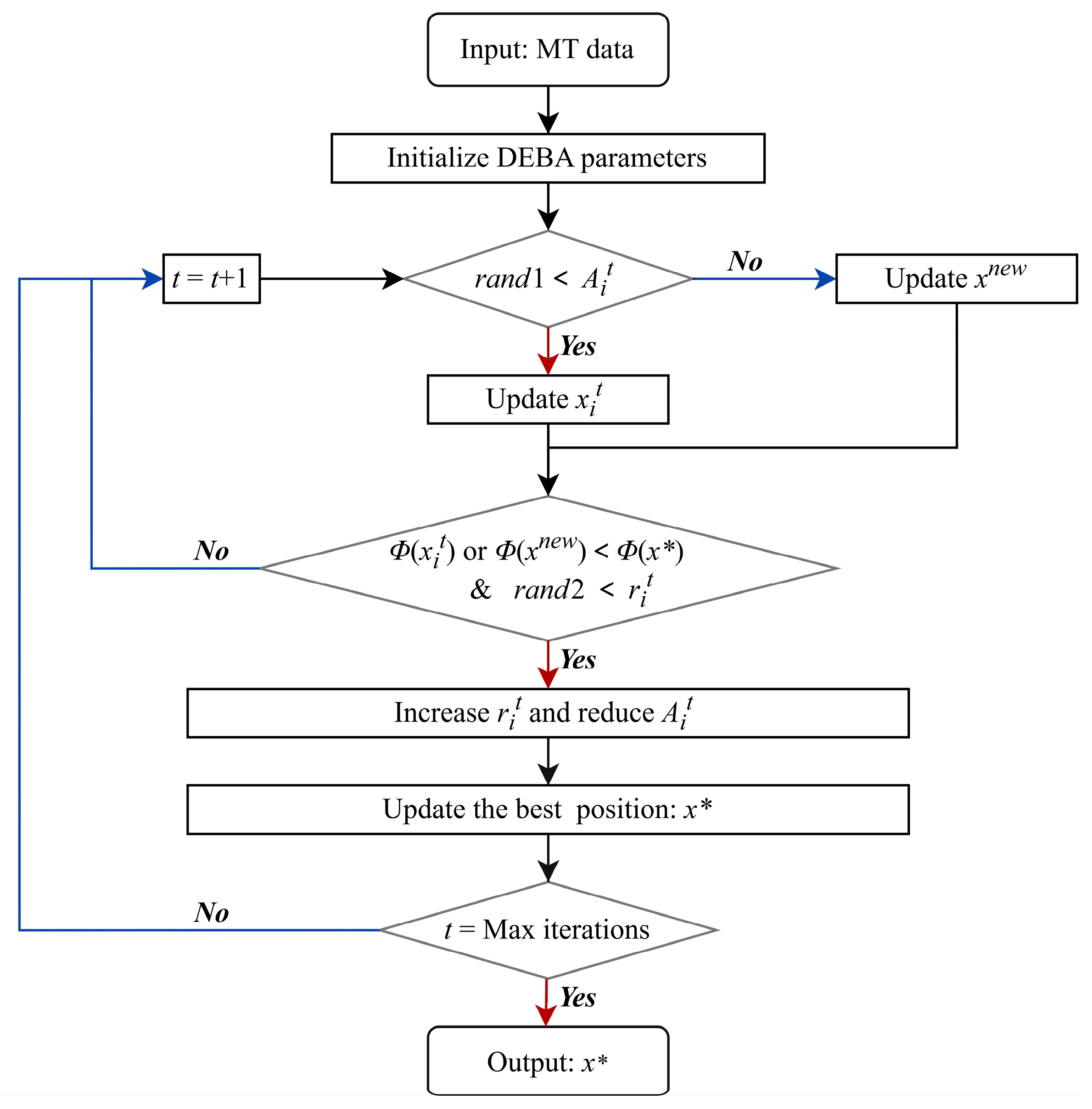
2.3. Improved DEBA Inversion
3. Model Test
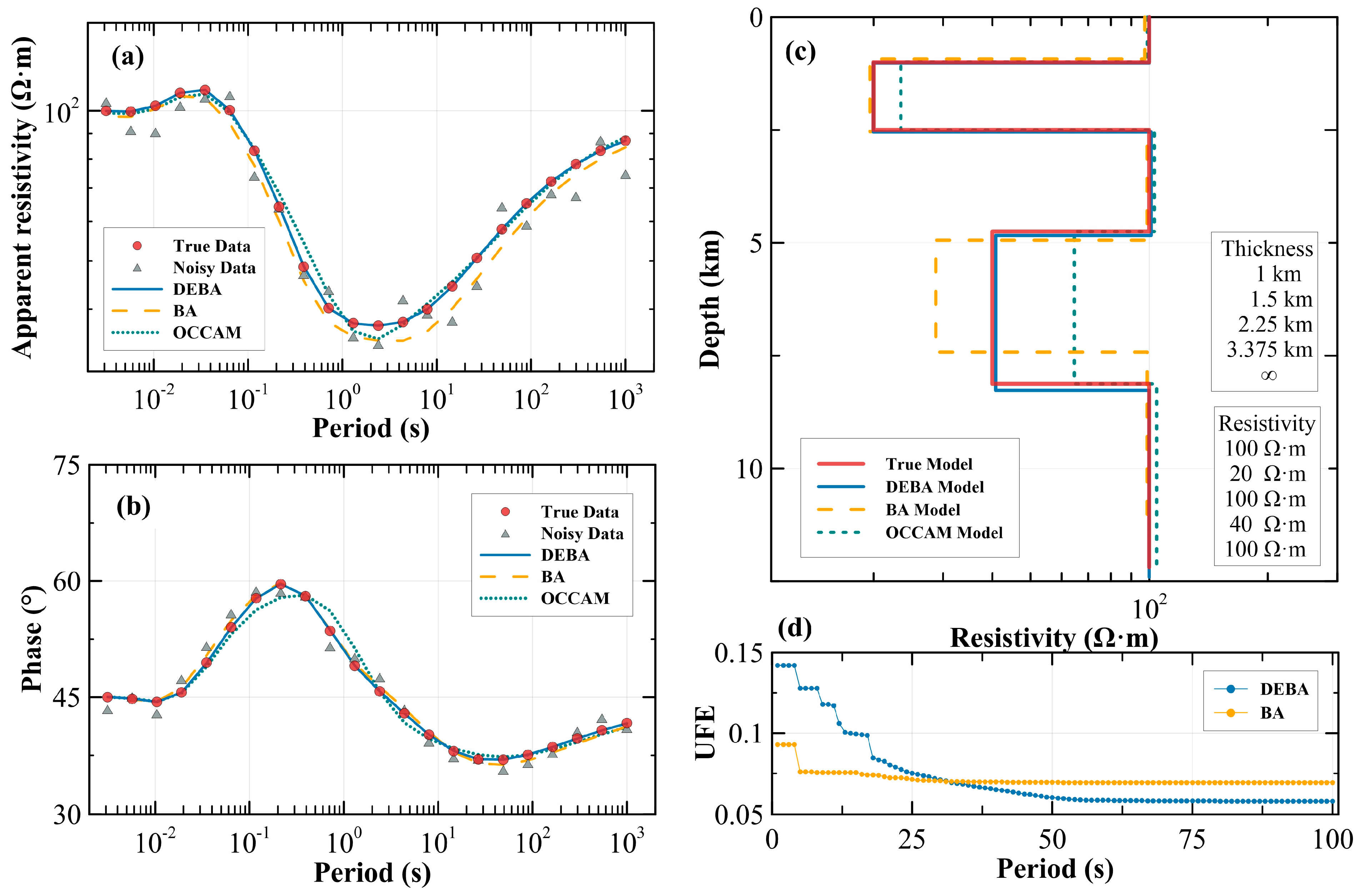
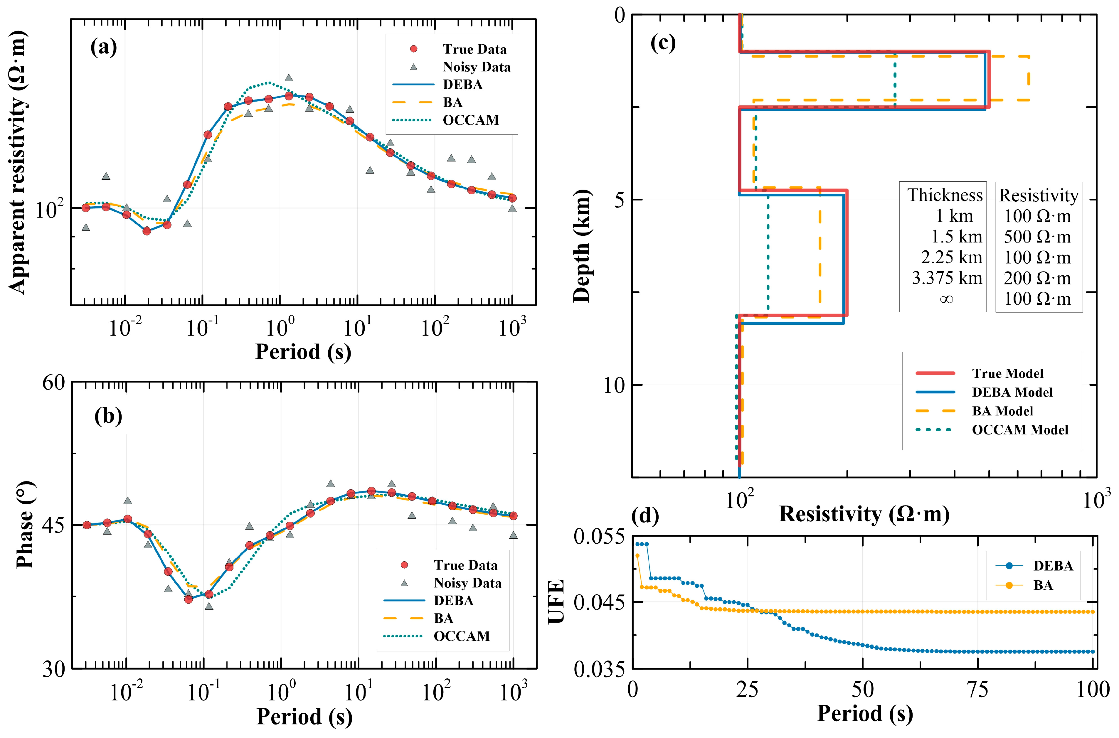
3.1. Numerical Test
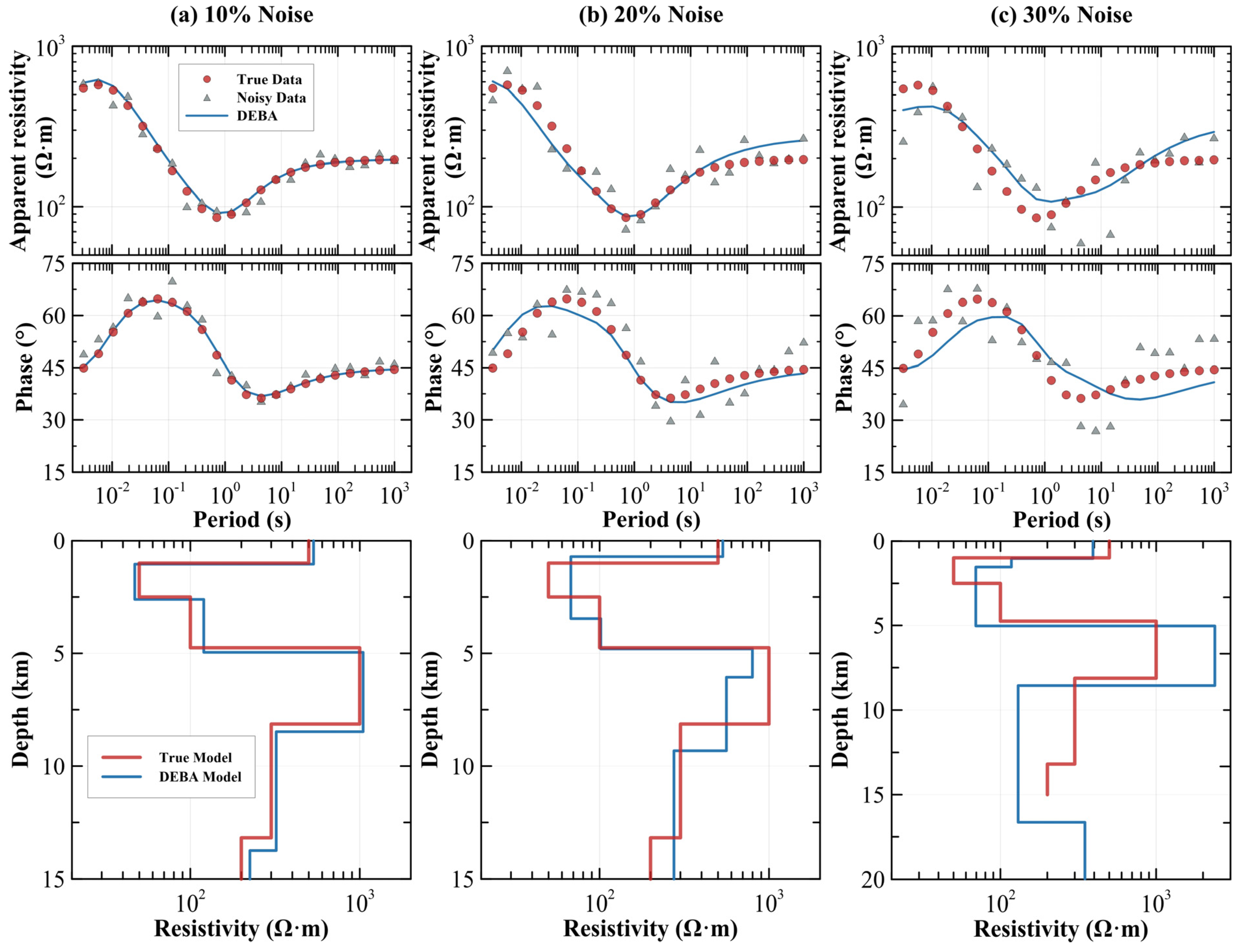
3.2. Noise Sensitivity Test
4. Evidence of Upper Crust Low-Resistivity Layers Beneath SLB
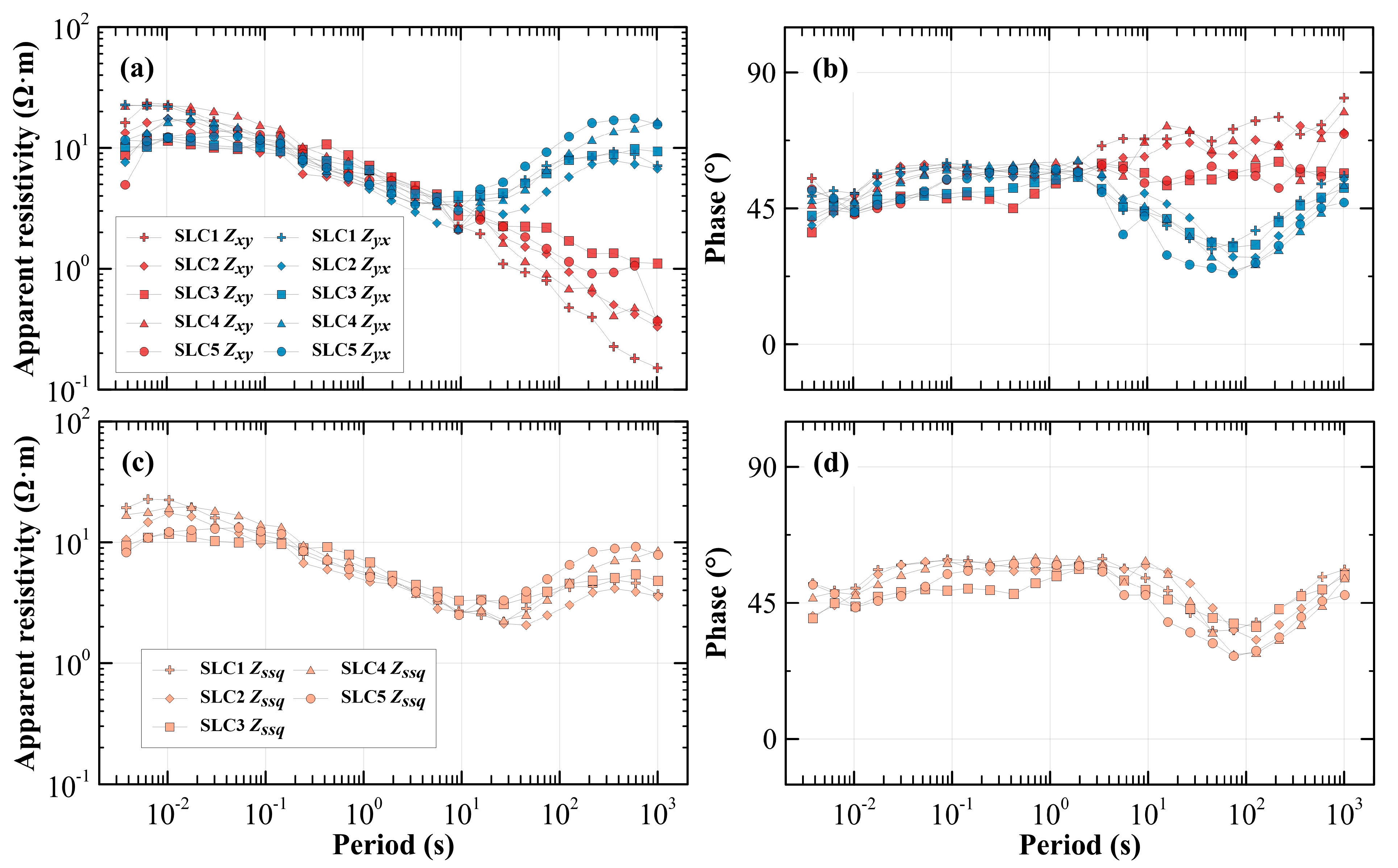
4.1. MT Data and Dimensionality Analysis
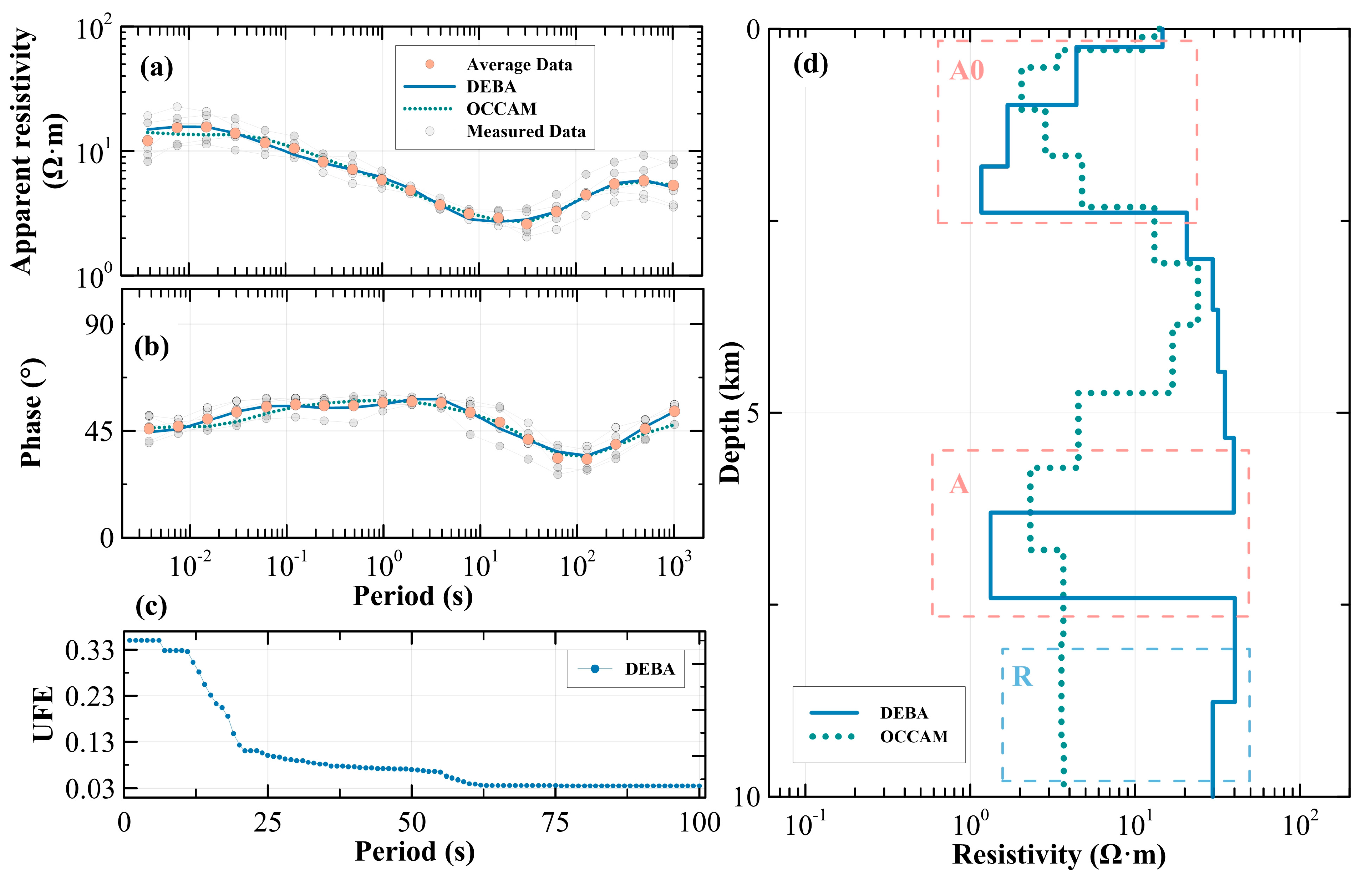
4.2. Results
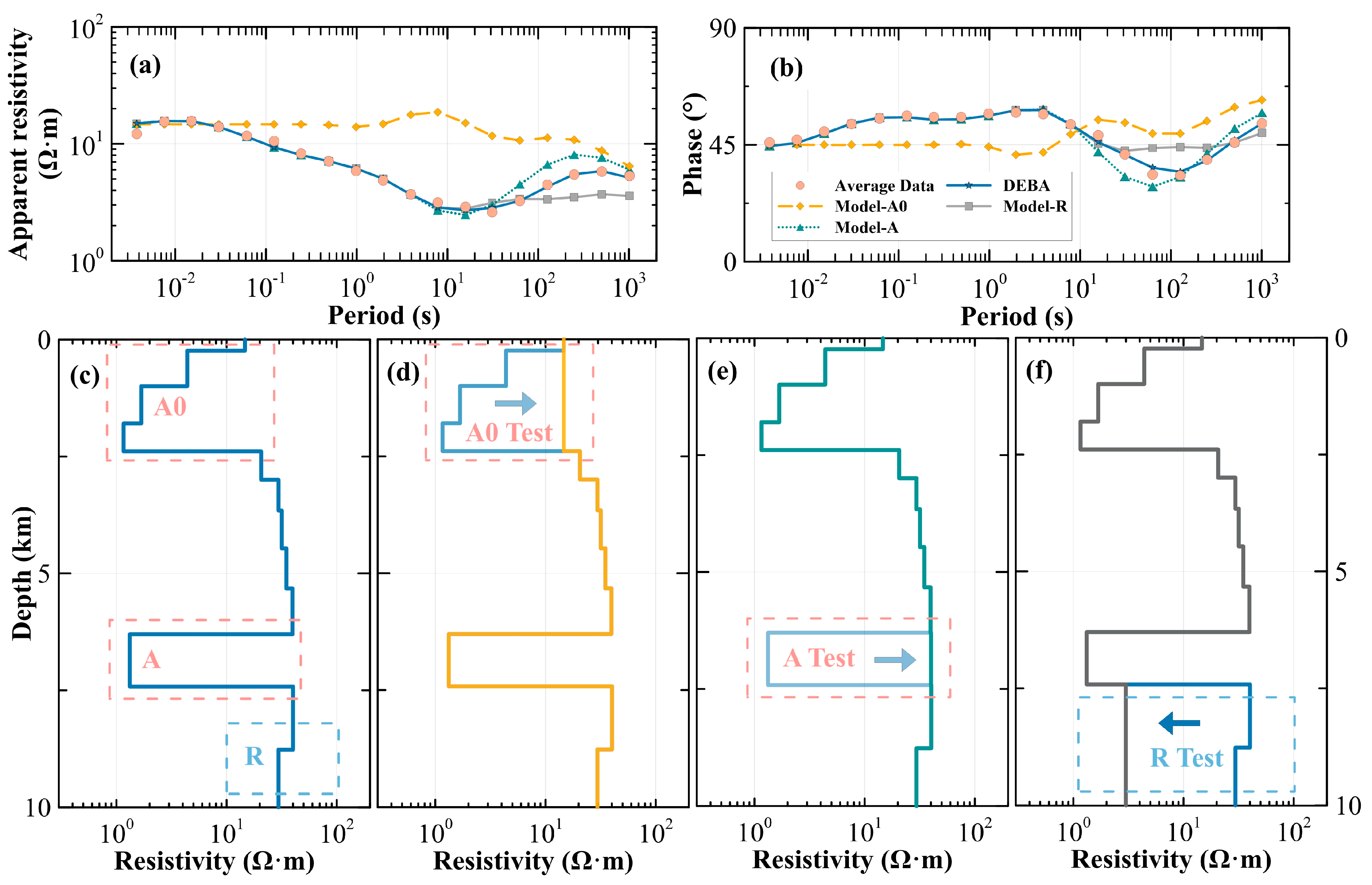
4.3. The Potential Causes of Low-Resistivity Anomaly A
5. Conclusions
Supplementary Materials
Author Contributions
Funding
Data Availability Statement
Acknowledgments
Conflicts of Interest
Abbreviations
| MT | Magnetotelluric |
| BBMT | Broadband magnetotelluric |
| SLB | Songliao Basin |
| DEBA | Dynamic Error Bat Algorithm |
| BA | Bat Algorithm |
| SA | Simulated Annealing |
| UFE | Uniform Fit Error |
| 1-D | One-dimensional |
| 2-D | Two-dimensional |
| 3-D | Three-dimensional |
References
- Jin, S.; Sheng, Y.; Liu, C.; Wei, W.; Ye, G.; Jing, J.; Zhang, L.; Dong, H.; Yin, Y.; Xie, C. A Review of Relationship between the Metallogenic System of Metallic Mineral Deposits and Lithospheric Electrical Structure: Insight from Magnetotelluric Imaging. Minerals 2024, 14, 541. [Google Scholar] [CrossRef]
- Li, Y.; Weng, A.; Xu, W.; Zou, Z.; Tang, Y.; Zhou, Z.; Li, S.; Zhang, Y.; Ventura, G. Translithospheric Magma Plumbing System of Intraplate Volcanoes as Revealed by Electrical Resistivity Imaging. Geology 2021, 49, 1337–1342. [Google Scholar] [CrossRef]
- Ma, C.; Li, B.; Li, J.; Wang, P.; Dong, J.; Cui, Z.; Yang, S. Characteristics and Deep Mineralization Prediction of the Langmuri Copper–Nickel Sulfide Deposit in the Eastern Kunlun Orogenic Belt, China. Minerals 2024, 14, 786. [Google Scholar] [CrossRef]
- Xu, D.; Zhang, Y.; Tang, B.; Yan, G.; Ye, G.; Dong, J.; Liu, B.; Zhang, Y. Three-Dimensional Electrical Structure and Metallogenic Background of the Southeastern Hubei Ore Concentration Area. Minerals 2024, 14, 558. [Google Scholar] [CrossRef]
- Ye, G.; Unsworth, M.; Wei, W.; Jin, S.; Liu, Z. The Lithospheric Structure of the Solonker Suture Zone and Adjacent Areas: Crustal Anisotropy Revealed by a High-Resolution Magnetotelluric Study. J. Geophys. Res. Solid Earth 2019, 124, 1142–1163. [Google Scholar] [CrossRef]
- Egbert, G.D.; Kelbert, A. Computational Recipes for Electromagnetic Inverse Problems. Geophys. J. Int. 2012, 189, 251–267. [Google Scholar] [CrossRef]
- Key, K. Marine Electromagnetic Studies of Seafloor Resources and Tectonics. Surv. Geophys. 2012, 33, 135–167. [Google Scholar] [CrossRef]
- Comeau, M.J.; Käufl, J.S.; Becken, M.; Kuvshinov, A.; Grayver, A.V.; Kamm, J.; Demberel, S.; Sukhbaatar, U.; Batmagnai, E. Evidence for Fluid and Melt Generation in Response to an Asthenospheric Upwelling beneath the Hangai Dome, Mongolia. Earth Planet. Sci. Lett. 2018, 487, 201–209. [Google Scholar] [CrossRef]
- Heagy, L.J.; Cockett, R.; Kang, S.; Rosenkjaer, G.K.; Oldenburg, D.W. A Framework for Simulation and Inversion in Electromagnetics. Comput. Geosci. 2017, 107, 1–19. [Google Scholar] [CrossRef]
- Castillo-Reyes, O.; de la Puente, J.; García-Castillo, L.E.; Cela, J.M. Parallel 3-D Marine Controlled-Source Electromagnetic Modelling Using High-Order Tetrahedral Nédélec Elements. Geophys. J. Int. 2019, 219, 39–65. [Google Scholar] [CrossRef]
- Zhi-qiang, F.; Cheng-zao, J.; Xi-nong, X.; Shun, Z.; Zi-hui, F.; Cross, T.A. Tectonostratigraphic Units and Stratigraphic Sequences of the Nonmarine Songliao Basin, Northeast China. Basin Res. 2010, 22, 79–95. [Google Scholar] [CrossRef]
- Feng, Z.; Zhang, S.; Feng, Z. Discovery of “Enveloping surface of oil and gas overpressure migration” in the Songliao Basin and its bearings on hydrocarbon migration and accumulation mechanisms. Sci. China Earth Sci. 2012, 55, 2005–2017. [Google Scholar] [CrossRef]
- Comeau, M.J.; Becken, M.; Kuvshinov, A.V. Imaging the Whole-Lithosphere Architecture of a Mineral System—Geophysical Signatures of the Sources and Pathways of Ore-Forming Fluids. Geochem. Geophys. Geosyst. 2022, 23, e2022GC010379. [Google Scholar] [CrossRef]
- Cai, H.; Zhdanov, M.S. Joint Inversion of Gravity and Magnetotelluric Data for the Depth-to-Basement Estimation. IEEE Geosci. Remote Sens. Lett. 2017, 14, 1228–1232. [Google Scholar] [CrossRef]
- Xie, C.; Jin, S.; Wei, W.; Ye, G.; Jing, J.; Zhang, L.; Dong, H.; Yin, Y.; Wang, G.; Xia, R. Crustal Electrical Structures and Deep Processes of the Eastern Lhasa Terrane in the South Tibetan Plateau as Revealed by Magnetotelluric Data. Tectonophysics 2016, 675, 168–180. [Google Scholar] [CrossRef]
- Smith, J.T.; Booker, J.R. Rapid Inversion of Two- and Three-Dimensional Magnetotelluric Data. J. Geophys. Res. Solid Earth 1991, 96, 3905–3922. [Google Scholar] [CrossRef]
- Gao, C.; Li, Y.; Wang, X. AUTL: An Attention U-Net Transfer Learning Inversion Framework for Magnetotelluric Data. IEEE Geosci. Remote Sens. Lett. 2024, 21, 3004505. [Google Scholar] [CrossRef]
- Jia, Z.; Li, Y.; Wang, Y.; Li, Y.; Jin, S.; Li, Y.; Lu, W. Deep Learning for 3-D Magnetic Inversion. IEEE Trans. Geosci. Remote Sens. 2023, 61, 5905410. [Google Scholar] [CrossRef]
- Yang, X.-S. A New Metaheuristic Bat-Inspired Algorithm; González, J.R., Pelta, D.A., Cruz, C., Terrazas, G., Krasnogor, N., Eds.; Springer: Berlin/Heidelberg, Germany, 2010; Volume 284, pp. 65–74. [Google Scholar]
- Wang, R.; Yin, C.; Wang, M.; Wang, G. Simulated Annealing for Controlled-Source Audio-Frequency Magnetotelluric Data Inversion. Geophysics 2012, 77, E127–E133. [Google Scholar] [CrossRef]
- Abdelazeem, M.; Emary, E.; Hassanien, A.E. A Hybrid Bat-Regularized Kaczmarz Algorithm to Solve Ill-Posed Geomagnetic Inverse Problem. In Proceedings of the 1st International Conference on Advanced Intelligent System and Informatics (AISI2015), Beni Suef, Egypt, 28–30 November 2015; Gaber, T., Hassanien, A.E., El-Bendary, N., Dey, N., Eds.; Springer International Publishing: Cham, Switzerland, 2016; pp. 263–272. [Google Scholar]
- Poormirzaee, R.; Sarmady, S.; Sharghi, Y. A New Inversion Method Using a Modified Bat Algorithm for Analysis of Seismic Refraction Data in Dam Site Investigation. J. Environ. Eng. Geophys. 2019, 24, 201–214. [Google Scholar] [CrossRef]
- Essa, K.S.; Diab, Z.E. Magnetic Data Interpretation for 2D Dikes by the Metaheuristic Bat Algorithm: Sustainable Development Cases. Sci. Rep. 2022, 12, 14206. [Google Scholar] [CrossRef]
- Yang, X.-S. Bat Algorithm: Literature Review and Applications. Int. J. Bio-Inspired Comput. 2013, 5, 141–149. [Google Scholar] [CrossRef]
- Cagniard, L. Basic Theory of the Magneto-telluric Method of Geophysical Prospecting. Geophysics 1953, 18, 605–635. [Google Scholar] [CrossRef]
- Tikhonov, T.A. On Determining Electrical Characteristics of the Deep Layers of the Earth’s Crust. Dokl. Akad. Nauk. SSSR 1950, 73, 295–297. [Google Scholar]
- Simpson, F.; Bahr, K. Practical Magnetotellurics; Cambridge University Press: Cambridge, UK, 2005; ISBN 978-0-521-81727-1. [Google Scholar]
- Rung-Arunwan, T.; Siripunvaraporn, W.; Utada, H. On the Berdichevsky Average. Phys. Earth Planet. Inter. 2016, 253, 1–4. [Google Scholar] [CrossRef]
- Gómez-Treviño, E.; Esparza Hernández, F.J.; Romo Jones, J.M. Effect of Galvanic Distortions on the Series and Parallel Magnetotelluric Impedances and Comparison with Other Responses. Geofís. Int. 2013, 52, 135–152. [Google Scholar] [CrossRef]
- Rung-Arunwan, T.; Siripunvaraporn, W.; Utada, H. Use of Ssq Rotational Invariant of Magnetotelluric Impedances for Estimating Informative Properties for Galvanic Distortion. Earth Planets Space 2017, 69, 80. [Google Scholar] [CrossRef]
- Newman, G.A.; Alumbaugh, D.L. Three-Dimensional Magnetotelluric Inversion Using Non-Linear Conjugate Gradients. Geophys. J. Int. 2000, 140, 410–424. [Google Scholar] [CrossRef]
- Kirkpatrick, S.; Gelatt, C.D.; Vecchi, M.P. Optimization by Simulated Annealing. In Readings in Computer Vision; Fischler, M.A., Firschein, O., Eds.; Morgan Kaufmann: San Francisco, CA, USA, 1987; pp. 606–615. ISBN 978-0-08-051581-6. [Google Scholar]
- Ren, J.; Tamaki, K.; Li, S.; Junxia, Z. Late Mesozoic and Cenozoic Rifting and Its Dynamic Setting in Eastern China and Adjacent Areas. Tectonophysics 2002, 344, 175–205. [Google Scholar] [CrossRef]
- Wang, T.; Ma, G.; Comeau, M.J.; Becken, M.; Zhou, Z.; Liu, W.; Kang, J.; Han, J. Evidence for the Superposition of Tectonic Systems in the Northern Songliao Block, NE China, Revealed by a 3-D Electrical Resistivity Model. J. Geophys. Res. Solid Earth 2022, 127, e2021JB022827. [Google Scholar] [CrossRef]
- Booker, J.R. The Magnetotelluric Phase Tensor: A Critical Review. Surv. Geophys. 2014, 35, 7–40. [Google Scholar] [CrossRef]
- Caldwell, T.G.; Bibby, H.M.; Brown, C. The Magnetotelluric Phase Tensor. Geophys. J. Int. 2004, 158, 457–469. [Google Scholar] [CrossRef]
- Jones, A.G.; Chave, A.D.; Egbert, G.; Auld, D.; Bahr, K. A Comparison of Techniques for Magnetotelluric Response Function Estimation. J. Geophys. Res. Solid Earth 1989, 94, 14201–14213. [Google Scholar] [CrossRef]
- Yadav, K.; Shah, M.; Sircar, A. Application of Magnetotelluric (MT) Study for the Identification of Shallow and Deep Aquifers in Dholera Geothermal Region. Groundw. Sustain. Dev. 2020, 11, 100472. [Google Scholar] [CrossRef]
- Chave, A.D.; Jones, A.G. (Eds.) The Magnetotelluric Method: Theory and Practice; Cambridge University Press: Cambridge, UK, 2012. [Google Scholar]
- Zhan, W.; Pan, L.; Chen, X. A Widespread Mid-Crustal Low-Velocity Layer beneath Northeast China Revealed by the Multimodal Inversion of Rayleigh Waves from Ambient Seismic Noise. J. Asian Earth Sci. 2020, 196, 104372. [Google Scholar] [CrossRef]
- Bai, D.; Unsworth, M.J.; Meju, M.A.; Ma, X.; Teng, J.; Kong, X.; Sun, Y.; Sun, J.; Wang, L.; Jiang, C.; et al. Crustal Deformation of the Eastern Tibetan Plateau Revealed by Magnetotelluric Imaging. Nat. Geosci. 2010, 3, 358–362. [Google Scholar] [CrossRef]
- Becken, M.; Ritter, O.; Bedrosian, P.A.; Weckmann, U. Correlation between Deep Fluids, Tremor and Creep along the Central San Andreas Fault. Nature 2011, 480, 87–90. [Google Scholar] [CrossRef]
- Li, S.; Weng, A.; Li, J.; Shan, X.; Han, J.; Tang, Y.; Zhang, Y.; Wang, X. Deep Origin of Cenozoic Volcanoes in Northeast China Revealed by 3-D Electrical Structure. Sci. China Earth Sci. 2020, 63, 533–547. [Google Scholar] [CrossRef]
- Tang, Y.; Weng, A.; Yang, Y.; Li, S.; Niu, J.; Zhang, Y.; Li, Y.; Li, J. Connection between Earthquakes and Deep Fluids Revealed by Magnetotelluric Imaging in Songyuan, China. Sci. China Earth Sci. 2021, 64, 161–176. [Google Scholar] [CrossRef]
- Wannamaker, P.E.; Caldwell, T.G.; Jiracek, G.R.; Maris, V.; Hill, G.J.; Ogawa, Y.; Bibby, H.M.; Bennie, S.L.; Heise, W. Fluid and Deformation Regime of an Advancing Subduction System at Marlborough, New Zealand. Nature 2009, 460, 733–736. [Google Scholar] [CrossRef]
- Watson, M.P.; Hayward, A.B.; Parkinson, D.N.; Zhang, Z.M. Plate Tectonic History, Basin Development and Petroleum Source Rock Deposition Onshore China. Mar. Pet. Geol. 1987, 4, 205–225. [Google Scholar] [CrossRef]
- Hyndman, R.D.; Vanyan, L.L.; Marquis, G.; Law, L.K. The Origin of Electrically Conductive Lower Continental Crust: Saline Water or Graphite? Phys. Earth Planet. Inter. 1993, 81, 325–345. [Google Scholar] [CrossRef]
- Selway, K. On the Causes of Electrical Conductivity Anomalies in Tectonically Stable Lithosphere. Surv. Geophys. 2014, 35, 219–257. [Google Scholar] [CrossRef]
- Yoshino, T.; Noritake, F. Unstable Graphite Films on Grain Boundaries in Crustal Rocks. Earth Planet. Sci. Lett. 2011, 306, 186–192. [Google Scholar] [CrossRef]
- Jiang, G.-Z.; Gao, P.; Rao, S.; Zhang, L.-Y. Compilation of heat flow data in the continental area of China (4th edition). Chin. J. Geophys. 2016, 59, 2892–2910. (In Chinese) [Google Scholar] [CrossRef]
- Sawyer, E.W.; Cesare, B.; Brown, M. When the Continental Crust Melts. Elements 2011, 7, 229–234. [Google Scholar] [CrossRef]
- Nover, G. Electrical Properties of Crustal and Mantle Rocks—A Review of Laboratory Measurements and Their Explanation. Surv. Geophys. 2005, 26, 593–651. [Google Scholar] [CrossRef]
- Sun, X.; Zhan, Y.; Zhao, L.; Xu, J.; Zhao, Y.; Zhao, B.; Yang, W. Does a Shallow Magma Reservoir Exist in the Wudalianchi Volcanic Field? Constraints From Magnetotelluric Imaging. Geophys. Res. Lett. 2023, 50, e2023GL104318. [Google Scholar] [CrossRef]
- Glover, P.W.J.; Hole, M.J.; Pous, J. A Modified Archie’s Law for Two Conducting Phases. Earth Planet. Sci. Lett. 2000, 180, 369–383. [Google Scholar] [CrossRef]
- Li, Y.; Weng, A.; Zhou, Z.; Guo, J.; Li, S.; Ventura, G.; Xu, W. Crustal Root Shapes the Plumbing System of a Monogenetic Volcanic Field as Revealed by Magnetotelluric Data. Earth Planet. Sci. Lett. 2024, 626, 118523. [Google Scholar] [CrossRef]
- Sinmyo, R.; Keppler, H. Electrical Conductivity of NaCl-Bearing Aqueous Fluids to 600 °C and 1 GPa. Contrib. Miner. Pet. 2017, 172, 4. [Google Scholar] [CrossRef]
- Kelbert, A.; Meqbel, N.; Egbert, G.D.; Tandon, K. ModEM: A Modular System for Inversion of Electromagnetic Geophysical Data. Comput. Geosci. 2014, 66, 40–53. [Google Scholar] [CrossRef]


Disclaimer/Publisher’s Note: The statements, opinions and data contained in all publications are solely those of the individual author(s) and contributor(s) and not of MDPI and/or the editor(s). MDPI and/or the editor(s) disclaim responsibility for any injury to people or property resulting from any ideas, methods, instructions or products referred to in the content. |
© 2025 by the authors. Licensee MDPI, Basel, Switzerland. This article is an open access article distributed under the terms and conditions of the Creative Commons Attribution (CC BY) license (https://creativecommons.org/licenses/by/4.0/).
Share and Cite
Qiao, S.; Yang, Y.; Zhou, Z.; Li, S.; Li, C.; Liu, X.; Wang, X. Dynamic Error Bat Algorithm: Theory and Application to Magnetotelluric Inversion. Minerals 2025, 15, 359. https://doi.org/10.3390/min15040359
Qiao S, Yang Y, Zhou Z, Li S, Li C, Liu X, Wang X. Dynamic Error Bat Algorithm: Theory and Application to Magnetotelluric Inversion. Minerals. 2025; 15(4):359. https://doi.org/10.3390/min15040359
Chicago/Turabian StyleQiao, Shuai, Yue Yang, Zikun Zhou, Shiwen Li, Chuncheng Li, Xiaoping Liu, and Xueqiu Wang. 2025. "Dynamic Error Bat Algorithm: Theory and Application to Magnetotelluric Inversion" Minerals 15, no. 4: 359. https://doi.org/10.3390/min15040359
APA StyleQiao, S., Yang, Y., Zhou, Z., Li, S., Li, C., Liu, X., & Wang, X. (2025). Dynamic Error Bat Algorithm: Theory and Application to Magnetotelluric Inversion. Minerals, 15(4), 359. https://doi.org/10.3390/min15040359