

Joint Inversion of Audio-Magnetotelluric and Dual-Frequency Induced Polarization Methods for the Exploration of Pb-Zn Ore Body and Alteration Zone in Inner Mongolia, China
 , ,
, ,  ,
,  , and
, and
Abstract
1. Introduction
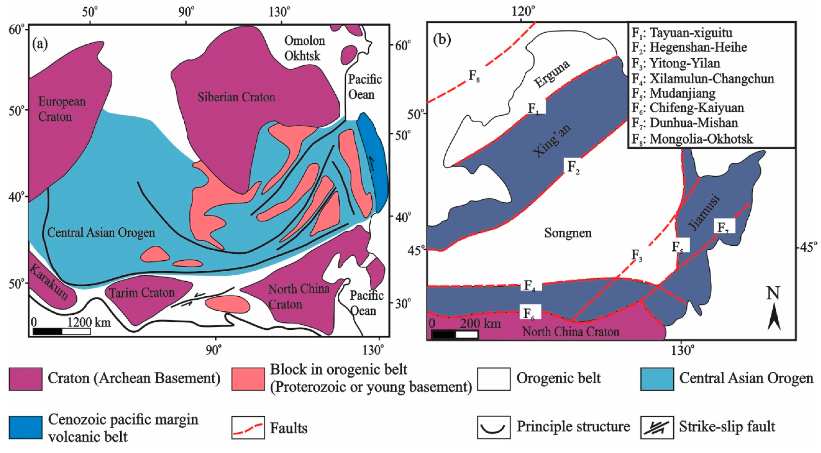
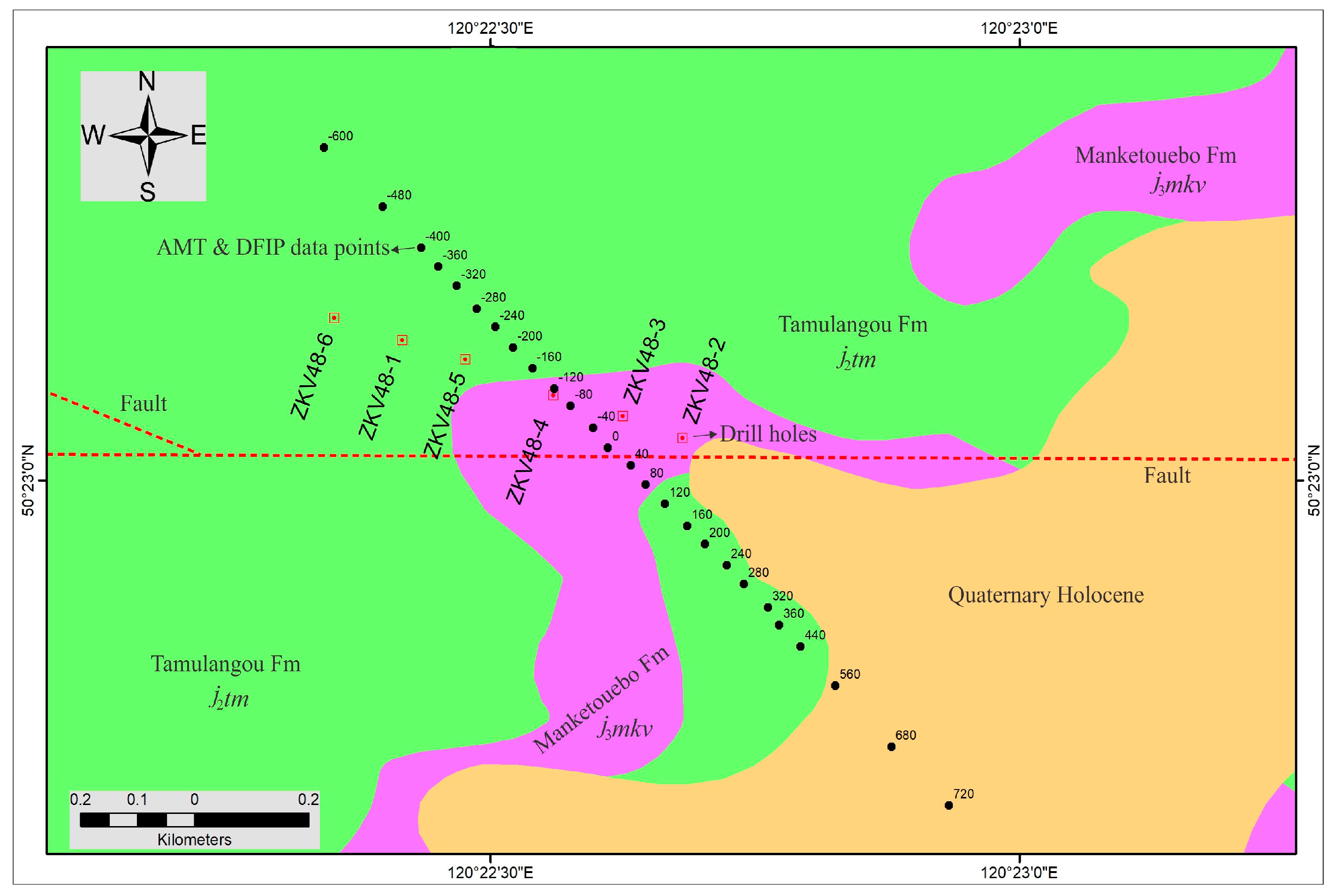
2. Regional Geology
3. Ore Deposit Geology
Mineralization and Alteration
4. Methodology, Data Acquisition, and Data Analysis
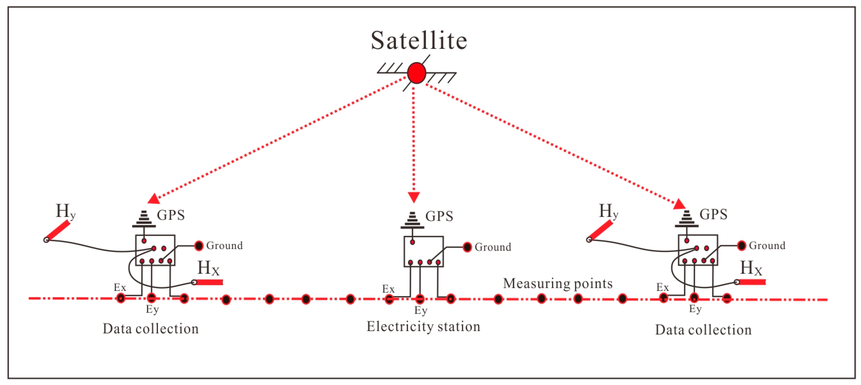
4.1. Audio Magnetotelluric (AMT) Method
4.2. Dual Frequency Induced Polarization Method
4.3. Data Acquisition
4.4. Data Analysis
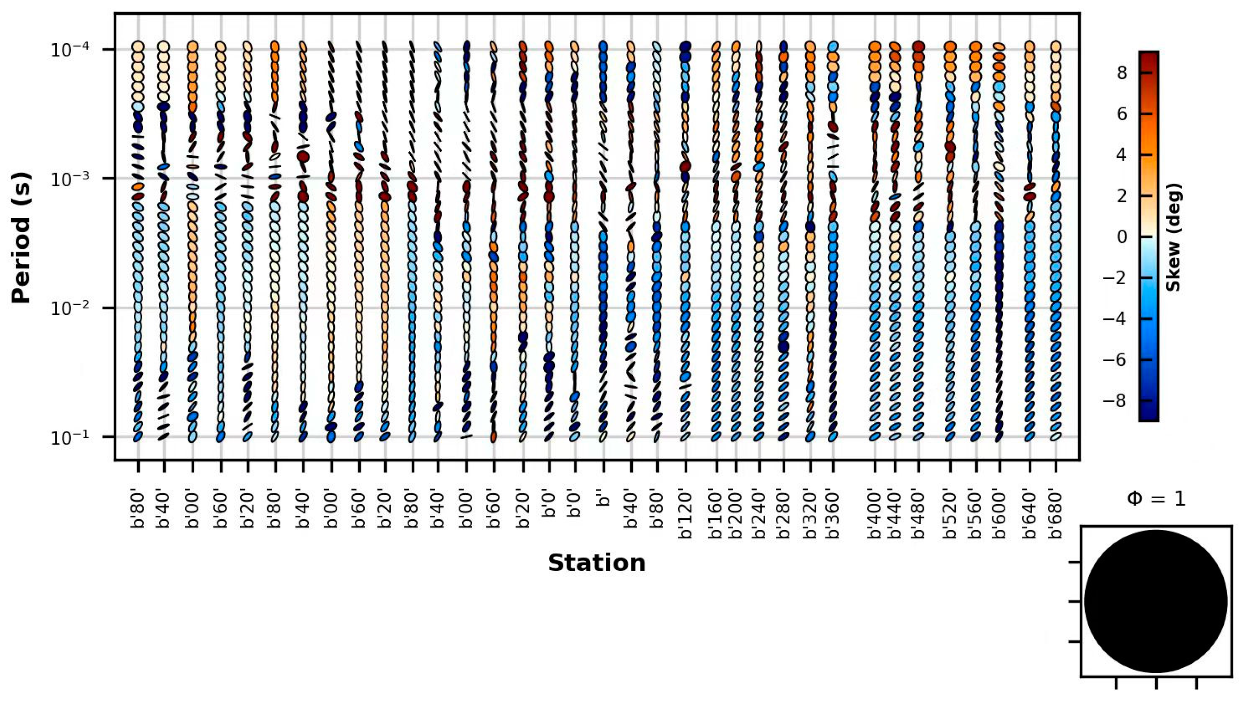
4.4.1. Dimensionality Analysis
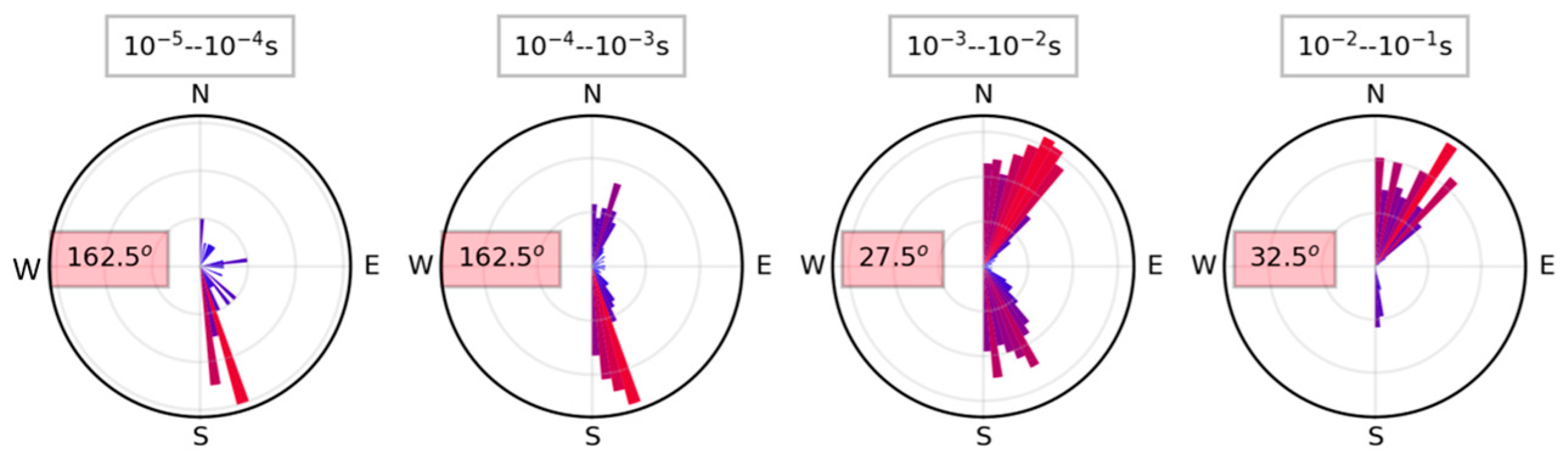
4.4.2. Geoelectric Strike Estimation
5. Inversion
5.1. AMT Data
5.2. DFIP Data
5.3. Joint Inversion Data
5.4. Inversion Results
5.4.1. AMT Result
5.4.2. DFIP Result
5.4.3. Joint Inversion Result
6. Discussion
7. Conclusions
Author Contributions
Funding
Data Availability Statement
Acknowledgments
Conflicts of Interest
References
- Gonzalez-Alvarez, I.; Goncalves, M.; Carranza, E.J.M. Introduction to the special issue challenges for mineral exploration in the 21st century: Targeting mineral deposits under cover. Ore Geol. Rev. 2020, 126, 103785. [Google Scholar] [CrossRef]
- Dan Wood, A.O.; Hedenquist, J. Mineral exploration: Discovering and defining ore deposits. SEG Newsl. 2019, 116, 1–22. [Google Scholar]
- Arnd, L.; Fo, Í.; Jeffrey, W.; Kesler, S.E.; Iel, G. D Future Global Mineral Resources. Geochem. Perspect. 2017, 6, 1. [Google Scholar] [CrossRef]
- Okada, K. Breakthrough technologies for mineral exploration. Miner. Econ. 2022, 35, 429–454. [Google Scholar] [CrossRef]
- Jiang, W.; Duan, J.; Doublier, M.; Clark, A.; Schofield, A.; Brodie, R.C.; Goodwin, J. Application of multiscale magnetotelluric data to mineral exploration: An example from the east Tennant region, Northern Australia. Geophys. J. Int. 2022, 229, 1628–1645. [Google Scholar] [CrossRef] [PubMed]
- Gan, J.; Li, H.; He, Z.; Gan, Y.; Mu, J.; Liu, H.; Wang, L. Application and significance of geological, geochemical, and geophysical methods in the Nanpo gold field in Laos. Minerals 2022, 12, 96. [Google Scholar] [CrossRef]
- McMillan, M.S.; Oldenburg, D.W. Cooperative constrained inversion of multiple electromagnetic data sets. Geophysics 2014, 79, B173–B185. [Google Scholar] [CrossRef]
- Bagchi, A.; Singh, R.K.; Sinharay, R.K. 3D Phase tensor inversion and Joint inversion using impedance and phase tensor components aiming better subsurface mapping and interpretation in Dhanjori basin, Singhbhum craton, eastern India. J. Appl. Geophys. 2022, 202, 104646. [Google Scholar] [CrossRef]
- Chen, R.; He, M.; Chang, F.; Zeng, P.; Zhao, X. Large-scale 3-D inversion of AMT data with application to mineral exploration. In Proceedings of the 23rd Electromagnetic Induction Workshop—EMIW 2016, Chiang Mai, Thailand, 20 August 2016; pp. 14–21. [Google Scholar]
- Ullah, F.; Zhou, X.; Chen, R.; Yang, L.; Yao, H.; Hu, H.; Chen, S.; Wang, Q. Cu–Polymetallic Deposit Exploration under Thick Cover in Gucheng–Yaxi Area Using Audio-Magnetotelluric and Spread-Spectrum-Induced Polarization. Minerals 2024, 14, 846. [Google Scholar] [CrossRef]
- Pitiya, R.; Lu, M.; Chen, R.; Nong, G.; Chen, S.; Yao, H.; Shen, R.; Jiang, E. Audio Magnetotellurics Study of the Geoelectric Structure across the Zhugongtang Giant Lead–Zinc Deposit, NW Guizhou Province, China. Minerals 2022, 12, 1552. [Google Scholar] [CrossRef]
- Kouabena, K.A.W. Enhancing prediction of deep-seated Cu-Mo porphyry deposit in Baohuashan: A comprehensive 2D inversion of AMT data. In Proceedings of the 26th EM Induction Workshop, Beppu, Japan, 7–13 September 2024. [Google Scholar]
- He, G.-L.; Wang, G.-J.; Zhou, C.; Yan, X.-L.; Li, H.-L. Application of Audio-frequency Magnetotelluric (AMT) in groundwater exploration: A case of the Nanmushui area in Zhanjiang. Prog. Geophys. 2019, 34, 304–309. [Google Scholar]
- Deshmukh, V.; Kumar, P.V.; Rao, P.S.; Kumar, A.; Singh, A. Audiomagnetotelluric (AMT) studies across Aravali-Tural-Rajawadi geothermal zones, western Maharastra, India. J. Appl. Geophys. 2022, 198, 104579. [Google Scholar] [CrossRef]
- Ishizu, K.; Ogawa, Y.; Mogi, T.; Yamaya, Y.; Uchida, T. Ability of the magnetotelluric method to image a deep conductor: Exploration of a supercritical geothermal system. Geothermics 2021, 96, 102205. [Google Scholar] [CrossRef]
- He, L.; Chen, L.; Dorji, X.X.; Zhao, X.; Chen, R.; Yao, H. Mapping the geothermal system using AMT and MT in the Mapamyum (QP) field, Lake Manasarovar, Southwestern Tibet. Energies 2016, 9, 855. [Google Scholar] [CrossRef]
- Wu, G.; Hu, X.; Huo, G.; Zhou, X. Geophysical exploration for geothermal resources: An application of MT and CSAMT in Jiangxia, Wuhan, China. J. Earth Sci. 2012, 23, 757–767. [Google Scholar] [CrossRef]
- Revil, A.; Vaudelet, P.; Su, Z.; Chen, R. Induced polarization as a tool to assess mineral deposits: A review. Minerals 2022, 12, 571. [Google Scholar] [CrossRef]
- Li, J. Application of the down-hole IP method to a general survey in the Jinya gold deposit. Geol. Explor. 2016, 52, 924–930. [Google Scholar]
- Ahmad, J.; Chen, R.; Ahmed, I.; Fahad, S.; Rahim, O.A.; Ullah, F.; Shah, S.A.; Li, R. Spread-spectrum induced polarization survey for Qiushuwan porphyry copper-molybdenum deposit in south of Henan Province, China. In Proceedings of the International Workshop on Gravity, Electrical & Magnetic Methods and Their Applications, Shenzhen, China, 19–22 May 2024; pp. 473–476. [Google Scholar]
- Ahmad, J.; Chen, R.; Ahmed, I.; Yaseen, M.; Shah, S.A.; Rahim, O.A.; Ullah, F.; Fahad, S.; Rui, L. Spread Spectrum Induced Polarization (SSIP) Survey for the Qiushuwan Copper–Molybdenum Deposits in Southern Henan Province, China. Minerals 2024, 14, 934. [Google Scholar] [CrossRef]
- Rahim, O.A.; Chen, R.; Liu, C.; El-Kaliouby, H.; Ahmed, I.; Ahmad, J.; Ullah, F.; Li, R.; Shah, S.A.; Fahad, S. Application of dual-frequency resistivity with forward and inverse pole-dipole array for groundwater exploration in Huarong County, Hunan, China. In Proceedings of the International Workshop on Gravity, Electrical & Magnetic Methods and Their Applications, Shenzhen, China, 19–22 May 2024; pp. 142–145. [Google Scholar]
- Ahmad, J. Comprehensive geophysical exploration of Shanshulin lead-zinc deposit in Laoyingshan town Guizhou, China. In Proceedings of the 26th EM Induction Workshop, Beppu, Japan, 7–13 September 2024. [Google Scholar]
- Kearey, P.; Brooks, M.; Hill, I. An Introduction to Geophysical Exploration; John Wiley & Sons: Hoboken, NJ, USA, 2002; Volume 4. [Google Scholar]
- Gallardo, L.A.; Meju, M.A. Joint two-dimensional DC resistivity and seismic travel time inversion with cross-gradients constraints. J. Geophys. Res. Solid Earth 2004, 109, B3. [Google Scholar] [CrossRef]
- Albouy, Y.; Andrieux, P.; Rakotondrasoa, G.; Ritz, M.; Descloitres, M.; Join, J.L.; Rasolomanana, E. Mapping coastal aquifers by joint inversion of DC and TEM soundings-three case histories. Groundwater 2001, 39, 87–97. [Google Scholar] [CrossRef]
- Vozoff, K.; Jupp, D. Joint inversion of geophysical data. Geophys. J. Int. 1975, 42, 977–991. [Google Scholar] [CrossRef]
- Haber, E.; Oldenburg, D. Joint inversion: A structural approach. Inverse Probl. 1997, 13, 63. [Google Scholar] [CrossRef]
- Linde, N.; Binley, A.; Tryggvason, A.; Pedersen, L.B.; Revil, A. Improved hydrogeophysical characterization using joint inversion of cross-hole electrical resistance and ground-penetrating radar traveltime data. In Water Resources Research; John Wiley & Sons: Hoboken, NJ, USA, 2006; Volume 42. [Google Scholar]
- Colombo, D.; De Stefano, M. Geophysical modeling via simultaneous joint inversion of seismic, gravity, and electromagnetic data: Application to prestack depth imaging. Lead. Edge 2007, 26, 326–331. [Google Scholar] [CrossRef]
- Wagner, D.; Koulakov, I.; Rabbel, W.; Luehr, B.-G.; Wittwer, A.; Kopp, H.; Bohm, M.; Asch, G.; Scientists, M. Joint inversion of active and passive seismic data in Central Java. Geophys. J. Int. 2007, 170, 923–932. [Google Scholar] [CrossRef]
- Sosa, A.; Velasco, A.A.; Velazquez, L.; Argaez, M.; Romero, R. Constrained optimization framework for joint inversion of geophysical data sets. Geophys. J. Int. 2013, 195, 1745–1762. [Google Scholar] [CrossRef]
- Moorkamp, M.; Jones, A.; Fishwick, S. Joint inversion of receiver functions, surface wave dispersion, and magnetotelluric data. J. Geophys. Res. Solid Earth 2010, 115, B4. [Google Scholar] [CrossRef]
- Zhdanov, M.S.; Jorgensen, M.; Cox, L. Advanced methods of joint inversion of multiphysics data for mineral exploration. Geosciences 2021, 11, 262. [Google Scholar] [CrossRef]
- Chen, B.; Jahn, B.-M.; Wilde, S.; Xu, B. Two contrasting Paleozoic magmatic belts in northern Inner Mongolia, China: Petrogenesis and tectonic implications. Tectonophysics 2000, 328, 157–182. [Google Scholar] [CrossRef]
- Xiao, W.; Windley, B.F.; Allen, M.B.; Han, C. Paleozoic multiple accretionary and collisional tectonics of the Chinese Tianshan orogenic collage. Gondwana Res. 2013, 23, 1316–1341. [Google Scholar] [CrossRef]
- Liang, H.-D.; Gao, R.; Hou, H.-S.; Liu, G.-X.; Han, J.-T.; Han, S. Lithospheric electrical structure of the Great Xing’an Range. J. Asian Earth Sci. 2015, 113, 501–507. [Google Scholar] [CrossRef]
- Chen, Z.; Zhang, L.; Wan, B.; Wu, H.; Cleven, N. Geochronology and geochemistry of the Wunugetushan porphyry Cu–Mo deposit in NE China, and their geological significance. Ore Geol. Rev. 2011, 43, 92–105. [Google Scholar] [CrossRef]
- Xiao, W.; Windley, B.F.; Hao, J.; Zhai, M. Accretion leading to collision and the Permian Solonker suture, Inner Mongolia, China: Termination of the central Asian orogenic belt. In Tectonics; John Wiley & Sons: Hoboken, NJ, USA, 2003; Volume 22. [Google Scholar]
- Wu, F.-Y.; Sun, D.-Y.; Ge, W.-C.; Zhang, Y.-B.; Grant, M.L.; Wilde, S.A.; Jahn, B.-M. Geochronology of the Phanerozoic granitoids in northeastern China. J. Asian Earth Sci. 2011, 41, 1–30. [Google Scholar] [CrossRef]
- Tang, J.; Xu, W.-L.; Wang, F.; Zhao, S.; Wang, W. Early Mesozoic southward subduction history of the Mongol–Okhotsk oceanic plate: Evidence from geochronology and geochemistry of Early Mesozoic intrusive rocks in the Erguna Massif, NE China. Gondwana Res. 2016, 31, 218–240. [Google Scholar] [CrossRef]
- Ouyang, H.-G.; Mao, J.-W.; Santosh, M.; Zhou, J.; Zhou, Z.-H.; Wu, Y.; Hou, L. Geodynamic setting of Mesozoic magmatism in NE China and surrounding regions: Perspectives from spatio-temporal distribution patterns of ore deposits. J. Asian Earth Sci. 2013, 78, 222–236. [Google Scholar] [CrossRef]
- Porter, T.M. The geology, structure and mineralisation of the Oyu Tolgoi porphyry copper-gold-molybdenum deposits, Mongolia: A review. Geosci. Front. 2016, 7, 375–407. [Google Scholar] [CrossRef]
- Ge, W.; Wu, F.; Zhou, C.; Zhang, J. Porphyry Cu-Mo deposits in the eastern Xing’an-Mongolian Orogenic Belt: Mineralization ages and their geodynamic implications. Chin. Sci. Bull. 2007, 52, 3416–3427. [Google Scholar] [CrossRef]
- Ge, W.-C.; Chen, J.-S.; Yang, H.; Zhao, G.-C.; Zhang, Y.-L.; Tian, D.-X. Tectonic implications of new zircon U–Pb ages for the Xinghuadukou Complex, Erguna Massif, northern Great Xing’an Range, NE China. J. Asian Earth Sci. 2015, 106, 169–185. [Google Scholar] [CrossRef]
- Xie, W.; Wen, S.; Zhang, G.; Tang, T. Geochronology, Fluid Inclusions and Isotopic Characteristics of the Dongjun Pb-Zn-Ag Deposit, Inner Mongolia, NE China. Acta Geol. Sin.-Engl. Ed. 2021, 95, 1611–1633. [Google Scholar] [CrossRef]
- Liu, J.; Mao, J.; Wu, G.; Wang, F.; Luo, D.; Hu, Y. Zircon U–Pb and molybdenite Re–Os dating of the Chalukou porphyry Mo deposit in the northern Great Xing’an Range, China and its geological significance. J. Asian Earth Sci. 2014, 79, 696–709. [Google Scholar] [CrossRef]
- Zhou, J.-B.; Wang, B.; Wilde, S.A.; Zhao, G.-C.; Cao, J.-L.; Zheng, C.-Q.; Zeng, W.-S. Geochemistry and U–Pb zircon dating of the Toudaoqiao blueschists in the Great Xing’an Range, northeast China, and tectonic implications. J. Asian Earth Sci. 2015, 97, 197–210. [Google Scholar] [CrossRef]
- Feng, Z.; Jia, J.; Liu, Y.; Wen, Q.; Li, W.; Liu, B.; Xing, D.; Zhang, L. Geochronology and geochemistry of the Carboniferous magmatism in the northern Great Xing’an Range, NE China: Constraints on the timing of amalgamation of Xing’an and Songnen blocks. J. Asian Earth Sci. 2015, 113, 411–426. [Google Scholar] [CrossRef]
- Duan, T.; Wen, S.; Zhou, P.; Zhu, E.; Cui, X.; Sun, J.; Zhao, T.; Wei, C. Wall Rock Alteration Characteristics and Mass Balance Calculation of Dongjun Pb-Zn-Ag Deposit in Inner Mongolia. J. Cent. South Univ. (Sci. Technol.) 2018, 49, 1991–2002. [Google Scholar]
- Liu, H.; Yang, X.; Yu, C.; Ye, J.; Liu, J.; Zeng, Q.; Shi, K. A case study in finding concealed ores by using geophysical exploration methods in combination of VLF-EM, EH4 and CSAMT. Prog. Geophys. 2004, 19, 276–285. [Google Scholar]
- Tikhonov, A. On determining electrical characteristics of the deep layers of the Earth’s crust. Dokl. Acad. Nauk. SSSR 1950, 73, 295–297. [Google Scholar]
- Cagniard, L. Basic theory of the magneto-telluric method of geophysical prospecting. Geophysics 1953, 18, 605–635. [Google Scholar] [CrossRef]
- Cantwell, T. Detection and Analysis of Low Frequency Magnetotelluric Signals. Ph.D. Thesis, Massachusetts Institute of Technology, Cambridge, MA, USA, 1960. [Google Scholar]
- Cantwell, T.; Madden, T. Preliminary report on crustal magnetotelluric measurements. J. Geophys. Res. 1960, 65, 4202–4205. [Google Scholar] [CrossRef]
- Vozoff, K. The magnetotelluric method in the exploration of sedimentary basins. Geophysics 1972, 37, 98–141. [Google Scholar] [CrossRef]
- Singh, R.K.; Maurya, V.P.; Singh, S. Imaging regional geology and Au–sulphide mineralization over Dhanjori greenstone belt: Implications from 3-D inversion of audio magnetotelluric data and petrophysical characterization. Ore Geol. Rev. 2019, 106, 369–386. [Google Scholar] [CrossRef]
- Ahmed, I.; Liu, H.; Chen, R.; Ahmad, J.; Shah, S.A.; Fahad, S.; Rahim, O.A.; Ullah, F.; Rui, L. Geothermal Resource Exploration in Reshi Town by Integrated Geophysical Methods. Energies 2024, 17, 856. [Google Scholar] [CrossRef]
- Tezkan, B. Radiomagnetotellurics. In Groundwater Geophysics: A Tool for Hydrogeology; Springer: Berlin/Heidelberg, Germany, 2009; pp. 295–317. [Google Scholar]
- Kalscheuer, T.; Juhojuntti, N.; Vaittinen, K. Two-dimensional magnetotelluric modelling of ore deposits: Improvements in model constraints by inclusion of borehole measurements. Surv. Geophys. 2018, 39, 467–507. [Google Scholar] [CrossRef]
- Chave, A.D.; Jones, A.G. The Magnetotelluric Method: Theory and Practice; Cambridge University Press: New York, NY, USA, 2012. [Google Scholar]
- Nabighian, M.N. Electromagnetic Methods in Applied Geophysics: Voume 1, Theory; Society of Exploration Geophysicists: Houston, TX, USA, 1988. [Google Scholar]
- Lindsay, M.; Spratt, J.; Occhipinti, S.; Aitken, A.; Dentith, M.; Hollis, J.; Tyler, I. Identifying mineral prospectivity using 3D magnetotelluric, potential field and geological data in the east Kimberley, Australia. Geol. Soc. Lond. Spec. Publ. 2018, 453, 247–268. [Google Scholar] [CrossRef]
- Li, F.; Zeng, Q.; Zhu, R.; Chu, S.; Xie, W.; Zhang, B.; Zhang, X. Application of the AMT Method to Gold Deposits: A Case Study in the Qinling Metallogenic Belt of North China Craton. Minerals 2021, 11, 1200. [Google Scholar] [CrossRef]
- Liu, W. Application of Dual Frequency IP Method in Southern Peru Copper Deposit Exploration. Adv. Mater. Res. 2012, 529, 311–317. [Google Scholar]
- He, J. Dual Frequency Induced Polarization Method; Higher Education Press: Beijing, China, 2006. [Google Scholar]
- Krieger, L.; Peacock, J.; Thiel, S.; Inverarity, K.; Robertson, K. MTpy: A Python Toolbox for Magnetotellurics. Comput. Geosci. 2014, 72, 167–175. [Google Scholar] [CrossRef]
- Booker, J.R. The magnetotelluric phase tensor: A critical review. Surv. Geophys. 2014, 35, 7–40. [Google Scholar] [CrossRef]
- Ren, W.; Ren, Z.; Xue, G.; Chen, W.; Zhao, P.; Liu, J. Three-dimensional audio magnetotelluric imaging of the Yangyi geothermal field in Tibet, China. J. Appl. Geophys. 2023, 211, 104966. [Google Scholar] [CrossRef]
- Weaver, J.T.; Agarwal, A.K.; Lilley, F. Characterization of the magnetotelluric tensor in terms of its invariants. Geophys. J. Int. 2000, 141, 321–336. [Google Scholar] [CrossRef]
- ZOND. ZondMT2D. 2001–2023. Available online: http://zond-geo.com/english/zond-software/electromagnetic-sounding/zondmt2d/ (accessed on 4 December 2023).
- ZOND. ZondRes2d. 2001–2023. Available online: http://zond-geo.com/english/zond-software/ert-and-ves/zondres2d/ (accessed on 4 December 2023).
- Gallardo, L.A.; Meju, M.A. Joint two-dimensional cross-gradient imaging of magnetotelluric and seismic traveltime data for structural and lithological classification. Geophys. J. Int. 2007, 169, 1261–1272. [Google Scholar] [CrossRef]
- Unsworth, M.; Egbert, G.; Booker, J. High-resolution electromagnetic imaging of the San Andreas fault in Central California. J. Geophys. Res. 1999, 104, 1131–1150. [Google Scholar] [CrossRef]


| Rock Ore Specimen | Resistivity Range ρ (Ω·m) | PFE (%) |
|---|---|---|
| Basalt | 1000~2000 | 0.7%~1.5% |
| Rhyolite | 1500~2800 | 0.5%~1.2% |
| Breccia | 2000~3000 | 0.3%~1.0% |
| Pb-Zn Ore | 500~1000 | ~15.0% |
Disclaimer/Publisher’s Note: The statements, opinions and data contained in all publications are solely those of the individual author(s) and contributor(s) and not of MDPI and/or the editor(s). MDPI and/or the editor(s) disclaim responsibility for any injury to people or property resulting from any ideas, methods, instructions or products referred to in the content. |
© 2025 by the authors. Licensee MDPI, Basel, Switzerland. This article is an open access article distributed under the terms and conditions of the Creative Commons Attribution (CC BY) license (https://creativecommons.org/licenses/by/4.0/).
Share and Cite
Fahad, S.; Liu, C.; Chen, R.; Ahmad, J.; Yaseen, M.; Shah, S.A.; Ullah, F.; Ahmed, I.; Rahim, O.A.; Li, R.; et al. Joint Inversion of Audio-Magnetotelluric and Dual-Frequency Induced Polarization Methods for the Exploration of Pb-Zn Ore Body and Alteration Zone in Inner Mongolia, China. Minerals 2025, 15, 287. https://doi.org/10.3390/min15030287
Fahad S, Liu C, Chen R, Ahmad J, Yaseen M, Shah SA, Ullah F, Ahmed I, Rahim OA, Li R, et al. Joint Inversion of Audio-Magnetotelluric and Dual-Frequency Induced Polarization Methods for the Exploration of Pb-Zn Ore Body and Alteration Zone in Inner Mongolia, China. Minerals. 2025; 15(3):287. https://doi.org/10.3390/min15030287
Chicago/Turabian StyleFahad, Shah, Chunming Liu, Rujun Chen, Jawad Ahmad, Muhammad Yaseen, Shahid Ali Shah, Farid Ullah, Ijaz Ahmed, Osama Abdul Rahim, Rui Li, and et al. 2025. "Joint Inversion of Audio-Magnetotelluric and Dual-Frequency Induced Polarization Methods for the Exploration of Pb-Zn Ore Body and Alteration Zone in Inner Mongolia, China" Minerals 15, no. 3: 287. https://doi.org/10.3390/min15030287
APA StyleFahad, S., Liu, C., Chen, R., Ahmad, J., Yaseen, M., Shah, S. A., Ullah, F., Ahmed, I., Rahim, O. A., Li, R., Mohamed, A. T., & El-Kaliouby, H. (2025). Joint Inversion of Audio-Magnetotelluric and Dual-Frequency Induced Polarization Methods for the Exploration of Pb-Zn Ore Body and Alteration Zone in Inner Mongolia, China. Minerals, 15(3), 287. https://doi.org/10.3390/min15030287