Article

Machine Learning-Based Mineral Quantification from Lower Cambrian Shale in the Sichuan Basin: Implications for Reservoir Quality

1
College of Geosciences, China University of Petroleum-Beijing, Beijing 102249, China
2
State Key Laboratory of Petroleum Resources and Engineering, China University of Petroleum-Beijing, Beijing 102249, China
3
Sinopec Petroleum Exploration & Production Research Institute, Beijing 100083, China
4
College of Energy, Chengdu University of Technology, Chengdu 610059, China
5
State Key Laboratory of Oil and Gas Reservoir Geology and Exploitation, Chengdu University of Technology, Chengdu 610059, China
6
Institute of Sedimentary Geology, Chengdu University of Technology, Chengdu 610059, China
*
Author to whom correspondence should be addressed.
Minerals 2025, 15(3), 286; https://doi.org/10.3390/min15030286
Submission received: 4 February 2025 / Revised: 26 February 2025 / Accepted: 3 March 2025 / Published: 12 March 2025

Abstract

:
In this study, cores from Well S1 in the Sichuan Basin were investigated to quantify mineral composition. A neural network analysis was employed to apply machine learning to X-ray fluorescence (XRF) datasets for predicting the mineralogical characteristics of Well S1. A total of 77 sample points were divided into training, validation, and test sets at a ratio of 6:2:2. After training and fine-tuning the model using the training and validation sets, the performance of the neural network model was evaluated with the test set. The best result was achieved for calcite prediction, reaching an R-squared (R2) value of 95%. Predictions for the seven minerals, except quartz, all exhibited R2 values of 80% or higher. Quantitative laboratory-measured X-ray diffraction (XRD) mineralogy was used for training to develop a high-resolution semi-quantitative model, and the resulting mineralogical model shows promising potential. The modeled mineralogy represents continuous relative abundance, which provides more meaningful insights compared to discrete single-point XRD measurements. The significance of this research lies in its ability to utilize relatively inexpensive and non-destructive XRF logging analysis, requiring minimal sample preparation, to construct high-resolution mineral abundance profiles. With modern technological advancements, operators can adopt the proposed method to build semi-quantitative mineralogical models for evaluating potential lateral drilling intervals and designing completion strategies accordingly.

1. Introduction

The characterization of organic-rich fine-grained rocks increasingly relies on handheld X-ray fluorescence (XRF) instruments, particularly for lithologies with limited visual differentiation potential, such as dark-colored mudstones [1,2]. These fine-grained lithologies present inherent challenges: their homogeneous texture obscures fabric details in core samples, while subtle geochemical variations often remain undetectable through conventional macroscopic analysis [3]. Modern handheld XRF technology addresses these limitations by capturing approximately 30 elemental signatures, enabling rapid identification of compositional trends that would otherwise require labor-intensive laboratory assays [4,5].
XRF measurements are cost- and time-efficient, requiring minimal sample preparation. The primary objective of this study is to develop a novel methodology for utilizing these elemental data to enable in-depth reservoir characterization and hydraulic fracturing modeling. In the proposed approach, seven major elements (Al, Ca, Fe, K, Mg, S, and Si) are employed to calculate the relative abundances of carbonate, quartz, feldspar, pyrite, and clay minerals, which constitute the dominant components of the rock matrix. The XRF elemental data were then calibrated against quantitative X-ray diffraction (XRD) measurements. We adopted artificial neural networks (ANNs) from the field of deep learning, adjusting model parameters such as the number of hidden layers and neurons per layer based on the training and validation sets to optimize the model’s ability to accurately predict the percentage content of each mineral in the test set. Machine learning (ML) and artificial intelligence (AI) have demonstrated significant potential in geological applications [6]. Examples include lithology identification and stratigraphic division using well-log data [7,8,9], the generation of high-resolution surface geological maps and mineral mapping through remote sensing techniques [10,11,12], and mineral composition analysis via X-ray diffraction (XRD) spectroscopy [13,14,15]. Despite these advancements, deriving continuous mineralogical compositions from X-ray fluorescence (XRF) elemental data remains challenging due to inherent limitations in data resolution and interpretive complexity [16,17]. This study specifically addresses two critical gaps in unconventional resource development: (1) the operational need for rapid mineralogical profiling during wellsite decision-making and (2) the economic imperative to reduce reliance on specialized laboratory analyses. By integrating ANN-based interpretation of XRF measurements with established XRD benchmarks, we establish a workflow that transforms elemental abundance data into actionable mineralogical intelligence. The developed methodology enables the generation of continuous mineral profiles at resolutions exceeding conventional laboratory sampling intervals (typically 30–100 cm) while maintaining 70%–80% cost reduction compared to traditional XRD-based approaches. Within the broader context of energy transition technologies, this advancement supports more sustainable exploitation of unconventional reservoirs through precision targeting of lateral sections and minimization of unnecessary hydraulic fracturing stages. Furthermore, the machine learning framework demonstrates how legacy core datasets can be revitalized through digital transformation, creating new value from historical geological archives that were previously underutilized due to analytical cost constraints.

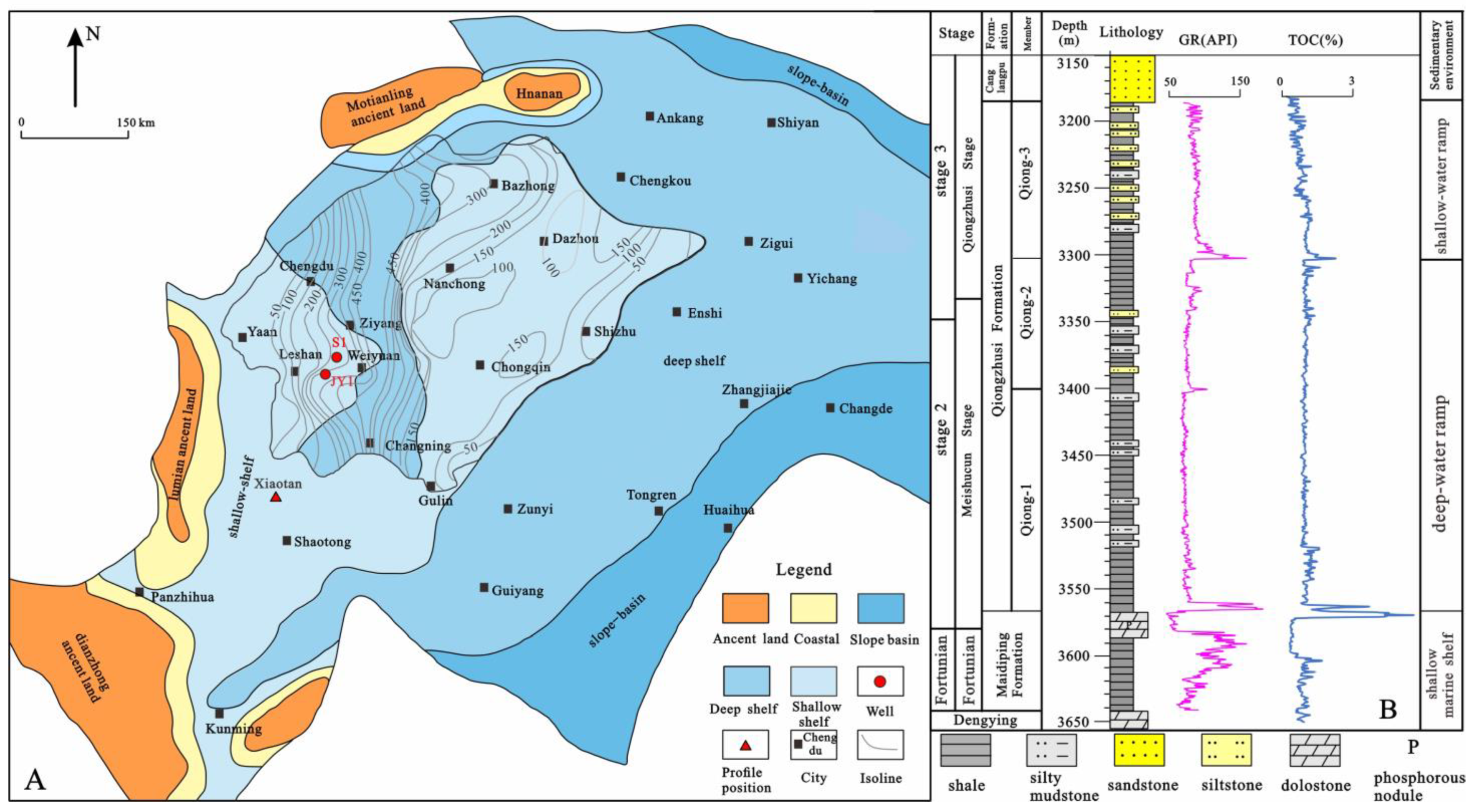
2. Geological Background

The late Neoproterozoic to early Cambrian tectonic evolution of the Yangtze Block was governed by the interplay between Rodinia supercontinent breakup and the Khingan rift system [18]. These processes triggered the fragmentation of the “Ancient China Craton”, generating north–south trending extensional troughs (e.g., Mianyang-Changning graben) and oceanic basins (e.g., Qinling-Tianshan) along reactivated Proterozoic sutures [19] (Figure 1A). Inherited Sinian deep-water depocenters in the Chengkou-E’xi transitional zone fostered a distinctive “shelf-trough-shelf” architecture [20], with debate persisting regarding the timing of rift initiation and sedimentary fill cyclicity [21]. Nevertheless, consensus holds that extensional tectonism spatially constrained Qiongzhusi Formation depocenters and hydrocarbon kitchens, while global eustatic rises during the Cambrian Explosion promoted widespread black shale deposition across the upper Yangtze Platform—a prerequisite for shale gas endowment [22,23,24].
Stratigraphic variability across the shelf trough system exerted first-order controls on shale depositional architecture, reservoir quality, and gas retention mechanisms. Isopach maps of the Lower Cambrian succession (Maidiping, Qiongzhusi, and Canglangpu Formations) reveal asymmetric trough geometry [25,26] involving maximum subsidence at northern and southern terminations versus central shallowing, with a gently dipping western flank contrasting the steep eastern margin bounded by syn-depositional faults. This structural grain-governed facies distribution involves the Leshan–Jingyan region (western trough slope), which is dominated by shallow-water ramp silty shales with low total organic carbon content (TOC average 0.41%), thicknesses of 320–380 m, and burial depths of 3200–4000 m. The Ziyang intra-trough domain is characterized by organic-rich deep-water ramp silty shales (TOC > 1%), thicknesses of 450–600 m, and burial depths of 4500–5000 m (Figure 1A).
The Qiongzhusi Formation comprises three upward-coarsening members (Qiong-1 to Qiong-3) (Figure 1B), each initiating with black organic-rich silty shales that grade into low-TOC muddy siltstones [27,28]. Stratigraphic completeness decreases troughward: Ziyang exhibits full succession preservation, whereas marginal Jingyan lacks upper intervals. Regionally, the unit transitions from phosphorite-bearing dolostones (underlying Maidiping Formation) to argillaceous siltstones (overlying Canglangpu Formation), recording progressive shallowing from Cambrian Stage 3 to Stage 4 [29].

3. Materials and Methods

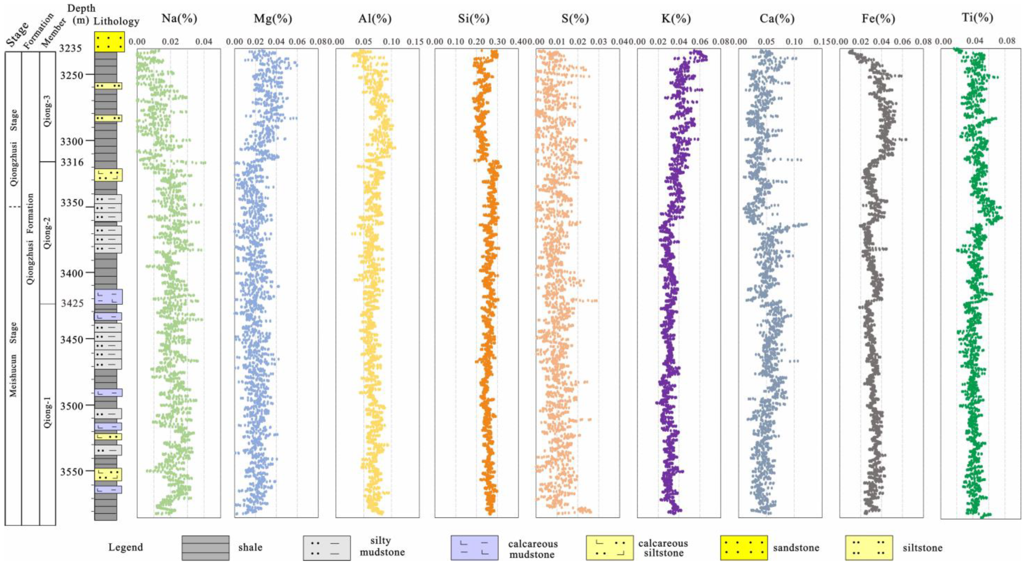
3.1. Geochemical Testing

Well S1, targeting the Qiongzhusi Formation in the Sichuan Basin, was selected to establish high-resolution geochemical composition models, with a focus on mineralogical reconstruction. Continuous core sampling spanning the 3300–3585 m interval was conducted at 20 cm resolution. Core surfaces were cleaned with ethanol and dried at 60 °C for 24 h prior to analysis to remove contaminants. Major element profiling utilized a Bruker AXS Tracer III-V handheld energy-dispersive XRF analyzer, operating at 15 kV excitation voltage, 0.15 mA current, and 60 s integration time per measurement (3 readings averaged per sample). Instrument calibration was verified daily using Montana soil and in-house shale reference materials, with analytical precision being confirmed through triplicate measurements. Following spectral calibration protocols outlined by Rowe et al. [30], 1339 discrete geochemical datasets were acquired along the borehole trajectory, constituting one of the densest XRF-derived geochemical inventories for Cambrian organic-rich shales in the basin (Figure 2).
Considering the lithology, depth, and major element characteristics of our samples, we selected 77 samples that cover as many of the existing mineralogical types as possible. Sample selection followed a stratified random sampling approach to ensure representation of all lithofacies types identified in preliminary core descriptions. Quantitative mineralogical validation was performed on 77 representative powdered samples through X-ray diffraction (XRD) analysis at the State Key Laboratory of Shale Oil and Gas Enrichment Mechanisms and Efficient Development (SINOPEC). Preparation involved dry grinding to <75 μm (200 mesh) using agate mortars to minimize iron contamination. Full-phase mineral quantification was achieved using a Bruker D8 Advance X-ray diffractometer, adhering to the Chinese petroleum industry standard SY/T 6210–1996 for mineral analysis. Each sample was analyzed in triplicate, with final mineral percentages calculated as the mean of three measurements (standard deviation < 2 wt.%). XRD patterns were acquired over a 2θ range of 5–70° with 0.02° step resolution, enabling precise identification of quartz, carbonates, and authigenic clay species (Table 1).

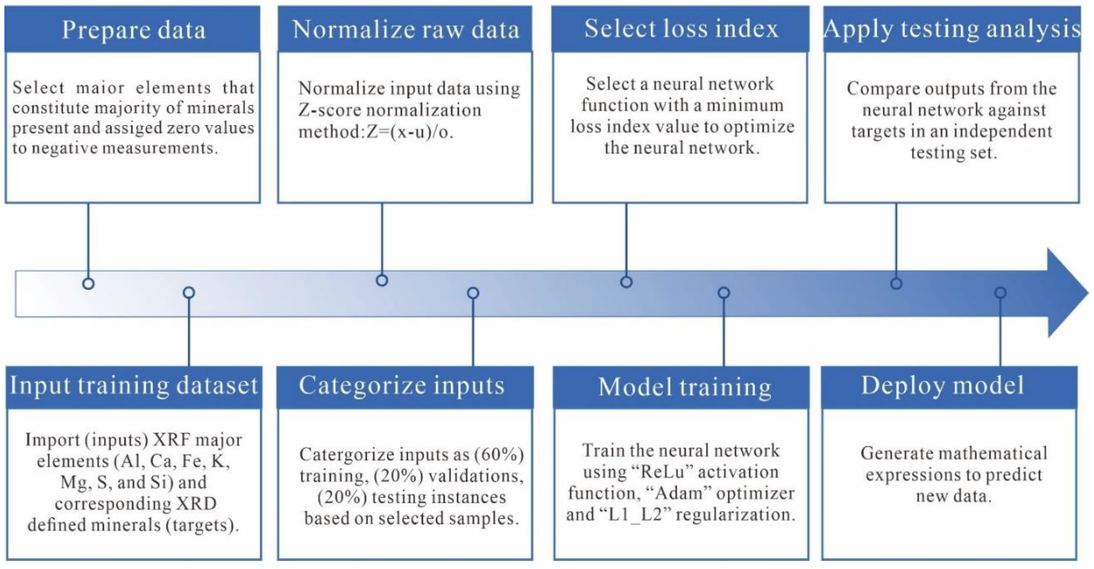
3.2. Methodology for Mineralogical Quantification

3.2.1. Data Preparation

The mineralogical quantification process followed a proposed workflow (Figure 3). The first step involved preparing the data for input into the software, with a thorough check for any missing values. Negative measurements were zero values, as negative concentrations are not physically meaningful. Such negative values can arise from various factors, including instrument detection limits and the duration of analysis, since elements at low concentrations require extended detection times [31]. In XRF analysis, the instrument provides a detection limit, representing the minimum element concentration that can be reliably measured. If the actual concentration of certain elements is below this detection limit, the XRF instrument may report a value below a specified threshold (e.g., <0.1%). For such values, we apply the following approach: if the value is >0.05%, we round it to 0.1%; if it is <0.05%, we assign it a value of 0. For values in the range of 0.1% to 100%, the measured data are typically used as is. For values exceeding the maximum detection limit (e.g., >100%), remeasurement of the sample and appropriate dilution methods may be necessary to ensure the data falls within the instrument’s measurable range. The XRD analysis revealed that the predominant minerals in the samples are quartz, K-feldspar, plagioclase, calcite, dolomite, pyrite, and clay minerals (Table S1). Figure 4 presents pie charts illustrating the mineral composition and the major elements (Al, Ca, Fe, K, Mg, Na, S, and Si) derived from XRF analysis. The elemental ratios shown in Figure 4 were calculated based on a generic chemical formula, with trace element substitutions being excluded for simplicity.

3.2.2. Input Training Dataset

Seventy-seven XRD analyses and corresponding XRF major elements were used to train, validate, and test the artificial neural network model we designed. To ensure statistical robustness, the dataset partitioning (60% training, 20% validation, 20% test) was repeated five times with random shuffling, and the results were averaged to minimize sampling bias [32]. Input variables included seven XRF-derived elements (Al, Ca, Fe, K, Mg, S, Si), while target outputs corresponded to six XRD-quantified minerals: calcite, dolomite, quartz, feldspar, pyrite, and clay minerals.

3.2.3. Normalizing Raw Data

Comprising major elements derived from an XRF analysis, underwent standardization to mitigate bias toward variables with larger magnitudes [33,34]. Z-score normalization was applied to rescale the input data to a mean of zero and a standard deviation of one. The Z-score represents the distance between an input value and the population mean in units of standard deviation [33]. For instance, calcium (Ca) normalization can be expressed as
Z = X μ σ
C a = C a 0.04 0.02
where X is the raw value, μ is the mean value, and σ is the standard deviation.

3.2.4. Categorizing Inputs

The dataset was partitioned into three subsets: (1) a training set (60%), (2) a validation set (20%), and (3) a test set (20%). This partitioning strategy is widely recommended, as it allocates most data for model optimization while retaining sufficient samples for unbiased evaluation [35]. The training subset was used to develop the predictive model, whereas the validation subset served to assess network generalizability, fine-tune hyperparameters, and halt training before overfitting occurred. The independent test subset evaluated the final model’s robustness [35]. In this study, the training, validation, and test subsets comprised 46, 16, and 15 samples, respectively.
Table 1 summarizes all 77 paired XRF-XRD samples. Input variables included seven XRF-derived elements (Al, Ca, Fe, K, Mg, S, Si), while target outputs corresponded to six XRD-quantified minerals: calcite, dolomite, quartz, feldspar, pyrite, and clay minerals. Figure 4 shows pie charts for these minerals and the major elements (from analysis) that compose the minerals. This figure is based on a generic chemical formula and, for simplicity, trace element substitutions were not considered (Figure 4). Due to analytical constraints in resolving individual clay species (e.g., illite vs. kaolinite), all clay minerals were grouped into a single category. Each mineral was modeled independently, as this approach yielded superior results compared to joint multi-mineral prediction. Input variable selection for each target mineral was governed by two criteria: (1) covariance between input and target and (2) minimization of the loss index (discussed in Section 3.3). Notably, training, validation, and test configurations varied across mineral models, as fixed partitioning resulted in elevated loss indices and suboptimal performance.

3.3. Model Tuning and Performance Evaluation

3.3.1. Loss Index Selection

Neural networks optimize by minimizing the loss function, which is a metric quantifying the cost of prediction errors [36]. In point estimation theory, the loss function quantifies the loss associated with parameter estimation errors. The expected loss (statistical risk) is commonly used to compare estimators, with lower expected loss indicating superior performance [37]. This study employed the Huber loss function, which combines the advantages of the mean absolute error (MAE) and mean squared error (MSE). While the MAE maintains constant gradients during training (risking convergence failure near minima), the MSE exhibits gradient decay near minima but amplifies outlier sensitivity. The Huber function mitigates both limitations, offering robustness against outliers while preserving stable convergence [38]. Training utilized the Rectified Linear Unit (ReLU) activation function and Adam optimizer [39] with L1 and L2 regularization to prevent overfitting [40]. This configuration achieved the lowest final training and validation losses. In addition, we incorporated strategies such as dropout and Early Stopping to prevent overfitting of the neural network model. For detailed algorithm comparisons, refer to [35]. Error minimization required the meticulous tuning of network architecture, including the number of hidden layers and neurons per layer. Figure 5 illustrates two representative architectures for calcite prediction. Both models share identical inputs but differ in hidden layer complexity. Increasing neurons enhances model capacity, potentially reducing errors at the cost of computational load. Optimal performance balances low training/validation losses with high test-set coefficient of determination (R2) (Figure 5). Example 1 in Figure 5 demonstrates superior performance (lower loss, higher R2, fewer iterations) despite simpler architecture. Activation functions, visualized as connecting lines between nodes, transform neuron outputs [41]. The Adam optimizer was selected based on empirical superiority in our simulations, aligning with findings by [41]. The ReLU served as an activation function to enable nonlinear transformations.

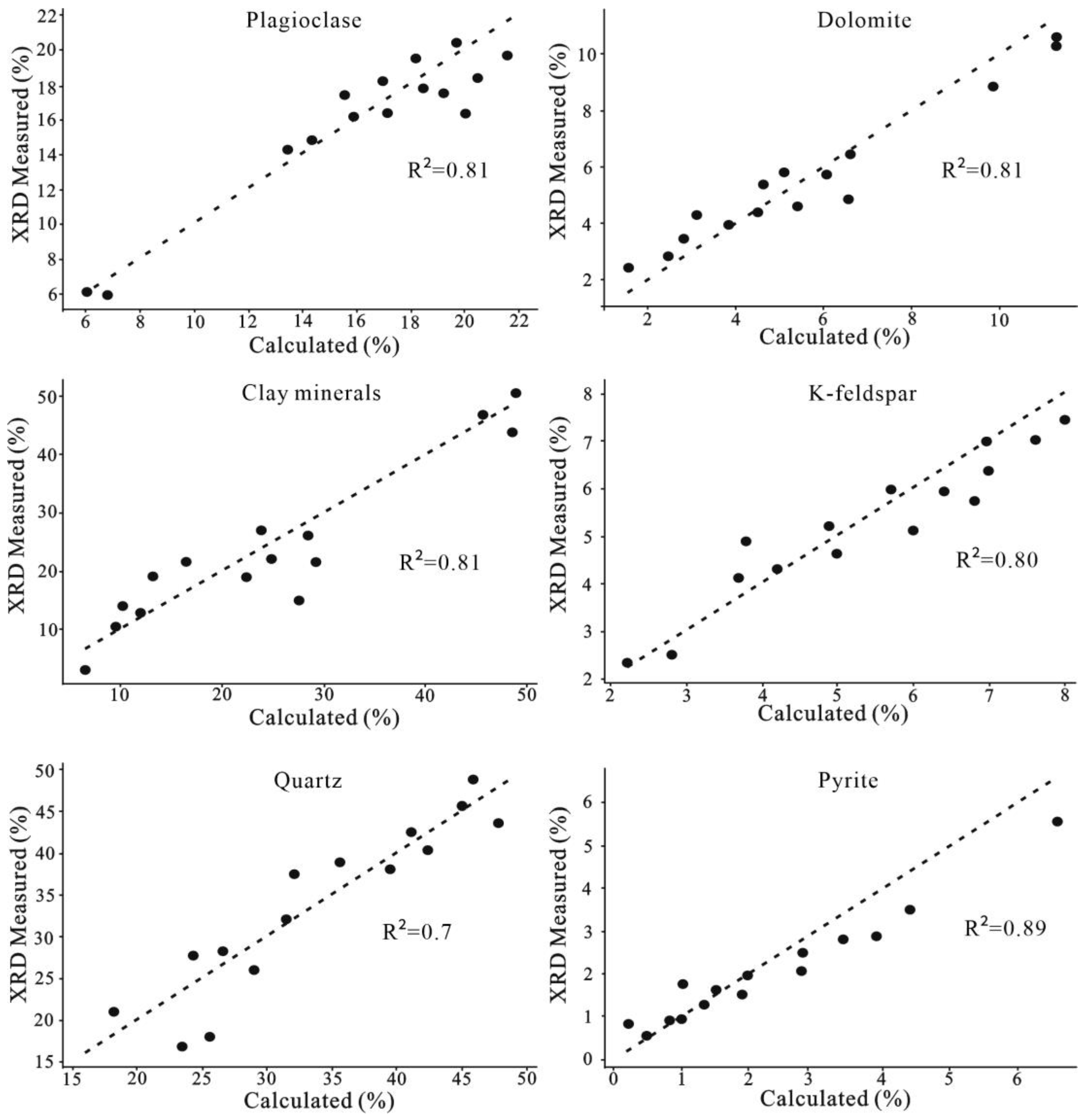
3.3.2. Performance Evaluation

The model iteratively trains on the training and validation subsets to identify the optimal model representation. Independent test instances, excluded from training, are then used to evaluate model generalizability by comparing neural network outputs (predicted mineralogy) against ground-truth XRD measurements. This comparative analysis is performed by plotting predicted versus measured mineral abundances, with model fidelity being assessed via the best-fit line slope (ideally 1.0) and the coefficient of determination (R2), which quantifies variance explained (Figure 6).
In the final phase, the validated model is deployed across the entire XRF dataset to predict mineral percentages at 20 cm resolution. By importing XRF geochemical profiles into the ANN model, high-resolution mineral logs for Well S1 are generated, enabling spatially continuous characterization of carbonate, quartz, and clay distributions (Figure 7 and Figure 8).

4. Results

4.1. Mineralogical Quantification

The training results of the mineralogical quantification in this study highlight the final training and validation loss values for each target (mineral) (Table 2). Both training and validation loss values significantly decreased with the increase in model iterations, which is the goal for a better model. To optimize the neural network model’s performance, we fine-tuned the model parameters for each mineral percentage prediction and selected the parameters that minimized the loss on both the training and validation sets. Figure 6 shows the linear regression analysis between the test instances (actual XRD results) and the neural network’s XRD outputs with the calcite model results referenced in Figure 5. From the model results, we observe that the R2 values for most mineral predictions are above 80%, with calcite and pyrite showing higher R2 values of 0.93 and 0.89, respectively. The R2 values for plagioclase, dolomite, and clay minerals are all 0.81. K-feldspar has an R2 of 0.80, while the prediction for quartz is the poorest, with an R2 of only 0.7. The dashed line in Figure 6 represents the line with a slope of 1 (y = x). The closer the points are to this line, the closer the predicted values are to the actual measured values, thus yielding a higher R2.

4.2. Geological Validation

Figure 7 and Figure 8 visually present the neural network-derived mineral composition profiles for Well S1, showing strong concordance between predicted mineral abundances (solid curves) and laboratory-validated XRD measurements (deep blue circles). The decision to partition results into two vertically consecutive plots stems from the high-density nature of the 77-sample dataset within the 285 m Qiongzhusi Shale interval. Figure 7 focuses on the upper 125 m, while Figure 8 details the lower 160 m, both maintaining identical vertical scaling (0.2 m resolution). This visualization strategy achieves dual objectives: (1) it prevents excessive data compression that would obscure critical mineralogical transitions across centimeter-scale laminae; (2) it enables clear discrimination of cyclical patterns in clay mineral content that correlate with gamma ray signatures.

5. Discussion

5.1. Technical Advantages

Our mineralogical estimation methodology demonstrates three key advantages. First, it generates high-resolution mineral logging (20 cm interval continuous profiles) with well-calibrated relative abundances, enabling precise identification of subtle mineralogical variations across centimeter-scale stratigraphic layers. Second, it integrates cost-effective XRF elemental data with targeted XRD point measurements that reduce reliance on expensive and labor-intensive XRD analyses—this dual-data synergy not only lowers operational costs but also enhances the interpretative power by leveraging XRF’s non-destructive and rapid sampling capabilities. Third, it preserves core integrity through non-destructive surface XRF sampling, creating opportunities for multidisciplinary analyses (e.g., geochemical, isotopic, or microbiological studies) that require intact core materials. Collectively, these advantages position our methodology as a versatile tool for high-precision mineral quantification in both exploration and production settings.

5.2. Current Limitations

While our methodology demonstrates notable advantages, it is important to acknowledge certain limitations and challenges. A minor limitation stems from the reliance on a relatively small XRD calibration dataset (n = 77), which could theoretically affect generalizability. However, this is partially mitigated by two key factors: first, deep-water depositional systems exhibit limited mineralogical variability due to diagenetic pathways, reducing the need for extensive sampling; second, we employed a multi-criteria sampling strategy that prioritized lithology, core descriptions, and elemental signatures to ensure representative coverage of mineral endmembers. Another technical consideration involves spatial discrepancies between XRF (core surface) and XRD (core interior) sampling, with samples collected from adjacent bedding planes (<20 cm apart). Despite potential minor compositional heterogeneities, their impact on model accuracy remains negligible given the lithological homogeneity within the Qiongzhusi Shale interval and the strong elemental–mineral correlations that dominate the training data.
Notably, quartz prediction exhibits the poorest performance (R2 = 0.7), primarily due to Si element interference—a challenge inherent in organic-rich shale systems where Si is shared among quartz, feldspars, and clay minerals. This interference is amplified by complex diagenetic interactions that complicate the isolation of quartz signals. To address these limitations and enhance methodological robustness, we propose three optimization strategies: (1) expanding the XRD dataset through multi-well collaborations to improve generalizability; (2) incorporating elemental ratios (e.g., Fe/Mg in clays) to strengthen mineral discriminability; and (3) applying transfer learning techniques to adapt the model to diverse depositional systems. Collectively, this methodology holds significant promise for high-resolution mineral mapping in unconventional reservoirs, non-destructive core analysis in offshore drilling operations, and paleoceanographic reconstruction via continuous mineral logs that distinguish detrital from authigenic mineral contributions.
XRF-derived major elements have proven valuable for characterizing sediment provenance (detrital vs. authigenic) and geological settings [42,43,44]. However, applications of XRF data to derive continuous mineralogical profiles remain sparse [45,46]. While this study focuses on the Qiongzhusi Formation and correlative units in the Sichuan Basin, it represents a critical advancement in quantifying mineralogical complexity within organic-rich shales. The open-source provision of input (XRF) and output (XRD) datasets (Table 2) establishes a foundational repository for future model refinement. Researchers are encouraged to augment this repository with additional calibrated data from other Qiongzhusi Formation wells, thereby enhancing predictive accuracy through expanded training populations.

6. Conclusions

(1)
Advancement in Mineralogical Analysis: This study marks a significant step forward in understanding the mineralogical composition of the Qiongzhusi Formation within the Sichuan Basin, utilizing neural network analysis to develop a machine learning-driven model for shale mineralogy.
(2)
Semi-Quantitative Methodology: The developed methodology offers a semi-quantitative approach to resolving complex mineral systems in the Qiongzhusi shales, providing continuous relative abundance profiles that add substantial interpretive value over discrete XRD measurements.
(3)
Framework for Data Integration: An initial framework has been established for integrating publicly available datasets with regional Lower Cambrian stratigraphic records, facilitating more comprehensive analyses and interpretations.
(4)
Operational Applications: The proposed semi-quantitative mineralogical approach enables operators to create predictive models during drilling operations by performing XRF analyses on core samples or drill cuttings, offering real-time mineralogical insights.

Supplementary Materials

The following supporting information can be downloaded at: https://www.mdpi.com/article/10.3390/min15030286/s1, Table S1: Major Element Composition by XRF Analysis.

Author Contributions

Conceptualization, X.Y. and Y.L.; investigation, T.H. and T.C.; software, T.H.; validation, X.Y.; formal analysis, Y.L. and S.L.; resources, X.Y.; data curation, T.H.; writing—original draft preparation, X.Y.; writing—review and editing, C.L.; visualization, S.J.; supervision, C.L.; project administration, S.L. and S.J.; funding acquisition, S.L. All authors have read and agreed to the published version of the manuscript.

Funding

This research was funded by the National Nature Science Foundation of China (42472180), Foundation of Key Laboratory of Deep-time Geography and Environment Reconstruction and Applications of Ministry of Natural Resources (DGERA20211102).

Data Availability Statement

Data are contained within the article.

Acknowledgments

Thanks for the great effort by the editors and reviewers.

Conflicts of Interest

Xin Ye is an employee of Sinopec Petroleum Exploration & Production Research Institute. The paper reflects the views of the scientists and not the company.

References

  1. Ryan, J.G.; Shervais, J.W.; Li, Y.; Reagan, M.K.; Li, H.Y.; Heaton, D.; Godard, M.; Kirchenbaur, M.; Whattam, S.A.; Pearce, J.A.; et al. The IODP Expedition 352 Scientific Team. Application of a handheld X-ray fluorescence spectrometer for real-time, high-density quantitative analysis of drilled igneous rocks and sediments during IODP Expedition 352. Chem. Geol. 2017, 451, 55–66. [Google Scholar] [CrossRef]
  2. Peng, J.; Larson, T.E. A Novel Integrated Approach for chemofacies characterization of organic-Rich mudrocks. AAPG Bull. 2022, 106, 437–460. [Google Scholar] [CrossRef]
  3. Pszonka, J.; Götze, J. Quantitative estimate of interstitial clays in sandstones using Nomarski differential interference contrast (DIC) microscopy and image analysis. J. Pet. Sci. Eng. 2018, 161, 582–589. [Google Scholar] [CrossRef]
  4. Gebregiorgis, D.; Giosan, L.; Hathorne, E.C.; Anand, P.; Nilsson-Kerr, K.; Plass, A.; Lückge, A.; Clemens, S.C.; Frank, M. What Can We Learn From X-Ray Fluorescence Core Scanning Data? A Paleomonsoon Case Study. Geochem. Geophys. Geosyst. 2020, 21, e2019GC008414. [Google Scholar] [CrossRef]
  5. Cao, H.Y.; Wang, H.; Zhao, R. The Application of the Handheld Energy-Dispersive X-Ray Fluorescence (ED-XRF) in the Cyclostratigraphy Research—A Case Study from the Xiagon Formation of the Lower Cretaceous in the Qingxi Sag, Jiuquan Basin. Earth Sci. 2017, 42, 2299–2311. [Google Scholar] [CrossRef]
  6. Pszonka, J.; Godlewski, P.; Fheed, A.; Dwornik, M.; Schulz, B.; Wendorff, M. Identificationand quantification of intergranular volume using SEM automated mineralogy. Mar. Pet. Geol. 2024, 162, 106708. [Google Scholar] [CrossRef]
  7. Jiang, C.; Zhang, D.; Chen, S. Lithology Identification from Well-Log Curves via Neural Networks with Additional Geologic Constraint. Geophysics 2021, 86, IMS85–IM100. [Google Scholar] [CrossRef]
  8. Zhang, J.; He, Y.; Zhang, Y.; Li, W.; Zhang, J. Well-Logging-Based Lithology Classification Using Machine Learning Methods for High-Quality Reservoir Identification: A Case Study of Baikouquan Formation in Mahu Area of Junggar Basin, NW China. Energies 2022, 15, 3675. [Google Scholar] [CrossRef]
  9. Rohit; Manda, S.R.; Raj, A.; Dheeraj, A.; Rawat, G.S.; Choudhury, T. Identification of Lithology from Well Log Data Using Machine Learning. EAI Endorsed Trans. Internet Things 2024, 10, 104605. [Google Scholar] [CrossRef]
  10. van der Meer, F.D.; van der Werff, H.M.A.; van Ruitenbeek, F.J.A.; Hecker, C.A.; Bakker, W.H.; Noomen, M.F.; van der Meijde, M.; Carranza, E.J.M.; de Smeth, J.B.; Woldai, T. Multi- and Hyperspectral Geologic Remote Sensing: A Review. Int. J. Appl. Earth Obs. Geoinf. 2012, 14, 112–128. [Google Scholar] [CrossRef]
  11. Harvey, A.; Fotopoulos, G. Geological Mapping Using Machine Learning Algorithms. Int. Arch. Photogramm. Remote Sens. Spat. Inf. Sci. 2016, 41, 423–430. [Google Scholar] [CrossRef]
  12. Honarmand, M.; Shahriari, H.; Zadeh, M.H.; Ghorbani, A. Enhancing Zn-bearing gossans from GeoEye-1 and Landsat 8 OLI data for non-sulphide Zn deposit exploration. Egypt. J. Remote Sens. Space Sci. 2024, 27, 93–107. [Google Scholar] [CrossRef]
  13. Sabins, F.F. Remote Sensing for Mineral Exploration. Ore Geol. Rev. 1999, 14, 157–183. [Google Scholar] [CrossRef]
  14. Ali, A.; Chiang, Y.W.; Santos, R.M. X-Ray Diffraction Techniques for Mineral Characterization: A Review for Engineers of the Fundamentals, Applications, and Research Directions. Minerals 2022, 12, 312. [Google Scholar] [CrossRef]
  15. Burkett, D.A.; Graham, I.T.; Ward, C.R. The Application of Portable X-Ray Diffraction to Quantitative Mineralogical Analysis of Hydrothermal Systems. Can. Mineral. 2015, 53, 429–454. [Google Scholar] [CrossRef]
  16. Alnahwi, A.; Loucks, R.G. Mineralogical Composition and Total Organic Carbon Quantification Using X-Ray Fluorescence Data from the Upper Cretaceous Eagle Ford Group in Southern Texas. AAPG Bull. 2019, 103, 2891–2907. [Google Scholar] [CrossRef]
  17. Chan, S.A.; Hassan, A.M.; Usman, M.; Humphrey, J.D.; Alzayer, Y.; Duque, F. Total Organic Carbon (TOC) Quantification Using Artificial Neural Networks: Improved Prediction by Leveraging XRF Data. J. Pet. Sci. Eng. 2022, 208 Pt E, 109302. [Google Scholar] [CrossRef]
  18. Li, Z.X. Tectonic history of the major East Asian lithospheric blocks since the Mid-Proterozoic—A synthesis. In Mantle Dynamics and Plate Interactions in East Asia; Flower, M.F.J., Chung, S.L., Lo, C.H., Eds.; American Geophysical Union: Washington, DC, USA, 1998; pp. 221–243. [Google Scholar] [CrossRef]
  19. Li, W.; Zhang, J.; Li, H.; Wang, X.; Zou, Q.; Jiang, H.; Fu, X.; Wang, P.; Xu, Z.; Ma, L. Distribution characteristics of intracratonic rift and its exploration significance in western Hubei and eastern Chongqing area. Nat. Gas Geosci. 2020, 31, 675–685. [Google Scholar] [CrossRef]
  20. Liu, S.; Sun, W.; Luo, Z.; Song, J.; Zhong, Y.; Tian, Y.; Peng, H. Xingkai taphrogenesis and petroleum exploration in the Lower Assemblage of Sichuan Basin. J. Chengdu Univ. Technol. (Sci. Technol. Ed.) 2013, 40, 511–520. [Google Scholar] [CrossRef]
  21. Liu, S.; Wang, Y.; Sun, W.; Zhong, Y.; Hong, H.; Deng, B.; Xia, M.; Song, J.; Ying, C.; Wu, J. Control of Intracratonic Sags on the Hydrocarbon Accumulations in the Marine Strata Across the Sichuan Basin, China. J. Chengdu Univ. Technol. (Sci. Technol. Ed.) 2016, 43, 1–23. [Google Scholar] [CrossRef]
  22. Li, D.; Ling, H.; Shields-Zhou, G.; Chen, X.; Cremonese, L.; Och, L.; Thirlwall, M.; Manning, C. Carbon and strontium isotope evolution of seawater across the Ediacaran–Cambrian transition: Evidence from the Xiaotan section, NE Yunnan, South China. Precambrian Res. 2013, 225, 128–147. [Google Scholar] [CrossRef]
  23. Zou, C.; Dong, D.; Wang, Y.; Li, X.; Huang, J.; Wang, S.; Guan, Q.; Zhang, C.; Wang, H.; Liu, H.; et al. Shale gas in China: Characteristics, challenges and prospects (I). Pet. Explor. Dev. 2015, 42, 753–767. [Google Scholar] [CrossRef]
  24. Zhao, J.; Jin, Z.; Lin, C.; Liu, G.; Liu, K.; Liu, Z.; Zhang, Y. Sedimentary Environment of the Lower Cambrian Qiongzhusi Formation Shale in the Upper Yangtze Region. Oil Gas Geol. 2019, 40, 701–715. [Google Scholar] [CrossRef]
  25. Wu, D.; Deng, H.; Xiong, L.; Cao, K.; Dong, X.; Zhao, Y.; Wei, L.; Wang, T.; Ma, R. Sequence filling and evolutionary model of the Lower Cambrian Maidiping Formation and Qiongzhusi Formation in the Sichuan Basin and its surrounding areas. Pet. Explor. Dev. 2023, 42, 753–767. [Google Scholar] [CrossRef]
  26. Xiong, L.; Deng, H.; Wu, D.; Wei, L.; Wang, T.; Zhou, H.; Cao, K.; Jie, X.; Ma, R.; Zhong, Y. Characteristics and influencing factors of fine-grained sedimentation in the Qiongzhusi Formation of the Lower Cambrian in the Sichuan Basin and its surrounding areas. Pet. Exp. Geol. 2023, 45, 857–871. [Google Scholar] [CrossRef]
  27. Yuan, Y.; Li, Y.; Fan, T.; Du, W.; Chen, G.; Zhang, T.; Kuang, M.; Liu, W. High-precision sequence stratigraphic characteristics and filling evolution model of fine-grained sedimentary rocks of the Lower Cambrian in the southwestern Sichuan region. Geosci. Front. 2023, 14, 162–180. [Google Scholar] [CrossRef]
  28. Luo, J.; Zhu, H.; Liang, X.; Liang, X.; Zhang, J.; Zhang, T.; Min, H.; Zhang, X.; Zou, C.; Li, J. Lithofacies paleogeography and distribution of high-quality shale of the Cambrian Qiongzhusi Formation in the Dianqianbei Depression. Acta Sedimentol. Sin. 2023, 41, 1257–1270. [Google Scholar] [CrossRef]
  29. He, X.; Liang, F.; Li, H.; Zheng, M.; Zhao, Q.; Liu, Y.; Liu, W. Breakthrough and enrichment mode of marine shale gas in the Lower Cambrian Qiongzhusi Formation in high-yield wells in Sichuan Basin. China Pet. Explor. 2024, 29, 142–155. [Google Scholar] [CrossRef]
  30. Rowe, H.; Hughes, N.; Robinson, K. The quantification and application of handheld energy-dispersive x-ray fluorescence (ED-XRF) in mudrock chemostratigraphy and geochemistry. Chem. Geol. 2012, 324-325, 122–131. [Google Scholar] [CrossRef]
  31. Adams, C.; Brand, C.; Dentith, M.; Fiorentini, M.; Caruso, S.; Mehta, M. The use of pXRF for light element geochemical analysis: A review of hardware design limitations and an empirical investigation of air, vacuum, helium flush and detector window technologies. Geochem. Explor. Environ. Anal. 2020, 20, 366–380. [Google Scholar] [CrossRef]
  32. Refaeilzadeh, P.; Tang, L.; Liu, H. Cross-Validation. Encycl. Database Syst. 2009, 1, 532–538. [Google Scholar] [CrossRef]
  33. Nawi, N.M.; Atomi, W.H.; Rehman, M.Z. The effect of data pre-processing on optimized training of artificial neural networks. Procedia Technol. 2013, 11, 32–39. [Google Scholar] [CrossRef]
  34. Meyer, F.O.; Price, R.C.; Al-Ghamdi, I.A.; Al-Goba, I.M.; Al-Raimi, S.M.; Cole, J.C. Sequential stratigraphy of outcropping strata equivalent to Arab-D reservoir, Wadi Nisah, Saudi Arabia. GeoArabia 1996, 1, 435–456. [Google Scholar] [CrossRef]
  35. Nguyen, G.H.; Bouzerdoum, A.; Phung, S.L. Learning pattern classification tasks with imbalanced data sets. Pattern Recognit. 2009, 10, 1322–1328. [Google Scholar]
  36. Zhao, H.; Gallo, O.; Frosio, I.; Kautz, J. Loss functions for image restoration with neural networks. IEEE Trans. Comput. Imaging 2016, 3, 47–57. [Google Scholar] [CrossRef]
  37. Prokudin, S.; Gehler, P.; Nowozin, S. Deep directional statistics: Pose estimation with uncertainty quantification. In Proceedings of the European Conference on Computer Vision (ECCV), Munich, Germany, 8–14 September 2018; pp. 534–551. [Google Scholar] [CrossRef]
  38. Xie, J.; Liu, S.; Chen, J.; Jia, J. Huber loss based distributed robust learning algorithm for random vector functional-link network. Artif. Intell. Rev. 2023, 56, 8197–8218. [Google Scholar] [CrossRef]
  39. Schmidt-Hieber, J. Nonparametric regression using deep neural networks with ReLU activation function. Ann. Stat. 2020, 48, 1875–1897. [Google Scholar] [CrossRef]
  40. Ying, X. An overview of overfitting and its solutions. J. Phys. Conf. Ser. 2019, 1168, 022022. [Google Scholar] [CrossRef]
  41. Szandała, T. Review and comparison of commonly used activation functions for deep neural networks. In Bio-Inspired Neurocomputing; Springer: Berlin/Heidelberg, Germany, 2021; pp. 203–224. [Google Scholar] [CrossRef]
  42. Rimmer, S.M. Geochemical paleoredox indicators in Devonian–Mississippian black shales, central Appalachian Basin (USA). Chem. Geol. 2004, 206, 373–391. [Google Scholar] [CrossRef]
  43. Pearce, C.R.; Cohen, A.S.; Coe, A.L.; Burton, K.W. Molybdenum isotope evidence for global ocean anoxia coupled with perturbations to the carbon cycle during the Early Jurassic. Geology 2008, 36, 231–234. [Google Scholar] [CrossRef]
  44. Mark, S.Z.; Abbott, M.B.; Rodbell, D.T.; Moy, C.M. XRF analysis of Laguna Pallcacocha sediments yields new insights into Holocene El Niño development. Earth Planet. Sci. Lett. 2022, 593, 117657. [Google Scholar] [CrossRef]
  45. Ross, P.S.; Bourke, A.; Fresia, B. Improving lithological discrimination in exploration drill-cores using portable X-ray fluorescence measurements: (1) testing three Olympus Innov-X analysers on unprepared cores. Geochem. Explor. Environ. Anal. 2014, 14, 171–185. [Google Scholar] [CrossRef]
  46. Löwemark, L.; Chen, H.F.; Yang, T.N.; Kylander, M.; Yu, E.; Hsu, Y.; Lee, T.; Song, S.; Jarvis, S. Normalizing XRF-scanner data: A cautionary note on the interpretation of high-resolution records from organic-rich lakes. J. Asian Earth Sci. 2011, 40, 1250–1256. [Google Scholar] [CrossRef]
Figure 1. (A) Tectonic–sedimentary framework of the Qiongzhusi Formation in Lower Cambrian during the depositional period; (B) composite stratigraphic column of the Qiongzhusi Formation shale from Well JY1.
Minerals 15 00286 g001
Figure 2. Major element content include Al, Ca, Fe, K, Mg, S and Si derived from an XRF analysis of the Well S1 core.
Minerals 15 00286 g002
Figure 3. A proposed workflow showing the steps followed in this study to quantify the mineralogy. Note that the mineralogy modeling uses the x-ray fluorescence elements Al, Ca, Fe, K, Mg, S and Si. During model training, we employ the Rectified Linear Unit (ReLU) activation function and the Adam optimizer, alongside L1 and L2 regularization, to prevent overfitting.
Minerals 15 00286 g003
Figure 4. Pie charts of dominant, existing minerals showing the XRF major elements that compose them, according to generic chemical formulas.
Minerals 15 00286 g004
Figure 5. Two examples of artificial neural network architecture for calcite are presented. Any neural network architecture must include input, output, and hidden layers. Neurons are connected to the input and output through activation functions, with the ReLU activation function being used in this study. Compared to Example 2, Example 1 demonstrates better fitting and overall final loss. Example 2 is more prone to overfitting, resulting in poorer performance on the test set. Minimizing the error requires fine-tuning the network’s structural parameters, such as the number of hidden layers and neurons in each layer. R2 represents the coefficient of determination; XRD stands for X-ray diffraction.
Minerals 15 00286 g005
Figure 6. The linear correlation plots between the predicted and measured values (XRD) for the other six mineral percentages in the test set. The closer the coefficient of determination (R2) is to 1, the better the model performance. The prediction results for quartz are the least accurate, with a coefficient of determination (R2) of 0.7.
Minerals 15 00286 g006
Figure 7. Calculated mineralogical abundance of core samples from Well S1, with a depth range of 3300–3425 m. Results for the Qiong-2 and Qiong-3 Member are presented, with deep blue circles indicating laboratory X-ray diffraction measurements. All trajectories are plotted to show the fit with the derived model.
Minerals 15 00286 g007
Figure 8. Calculated mineralogical abundance of core samples from Well S1, with a depth range of 3425–3585 m. Results for the Qiong-1 Member are presented, with deep blue circles representing laboratory X-ray diffraction measurements. All trajectories are plotted to show the fit with the derived model.
Minerals 15 00286 g008
Table 1. XRF data used for model input and XRD data used for output.
Input: XRF Elemental Data, %Targets: XRD Mineralogical Data, %
Depth
(m)
FeAlCaMgSSiKQuartzK-FeldsparPlagioclaseCalciteDolomitePyriteClay Minerals
Qiong-33314.794.18.91.83.81.722.64.32825.42.311.32.448.6
3315.824.18.12.44.11.322.63.928.92.26.14.411.31.645.5
3317.653.76.29.42.21.320.4429.62.56.42.17.53.348.6
3317.993.65.7112.11.619.23.8312.46.82.17.44.346
3319.153.26.91.51.81.829.73.540.93.912.92.07.21.831.3
3320.293.78.12.50.02.029.43.842.95.112.82.76.71.528.3
3322.192.86.02.72.40.628.92.943.04.1142.56.01.229.2
3325.272.57.04.42.61.425.54.046.93.812.64.48.81.522
3328.812.48.32.61.31.428.23.645.14.214.836.61.025.3
3330.422.67.43.32.10.927.13.443.63.914.72.94.61.928.4
3332.203.07.02.41.40.629.63.546.54.213.81.95.60.927.1
3333.103.17.54.00.80.827.83.350.04.316.73.05.41.918.7
3339.212.76.65.20.80.628.03.237.96.619.03.05.81.026.7
3342.322.95.35.32.11.227.03.343.97.218.33.23.82.321.3
3345.573.46.93.41.91.127.13.845.47.115.96.64.40.819.8
3347.383.66.93.60.51.728.73.540.45.718.72.76.40.925.2
3348.6145.94.42.21.626.13.9324.619.913.83.41.524.8
3350.153.15.84.41.70.128.13.538.64.721.65.14.23.422.4
3351.903.47.32.82.61.626.43.132.36.61710.73.91.528
3353.873.76.23.60.8029.23.642.55.6191.74.80.226.2
3355.103.47.81.12.80.727.33.152.15.518.12.930.318.1
3356.123.46.32.52.30.428.22.947.26.416.51.34.20.424
3356.783.87.42.71.71.427.43.247.76.518.81.63.30.321.8
3358.3247.41.82.31.427.32.850.55.515.72.52.70.422.7
3360.874.14.92.42.71.328.83.646.85.517.323.10.524.8
3361.703.65.92.71.90.528.93.546.95.718.22.12.63.521
3363.123.44.82.63.5028.23.546.15.517.22.53.70.624.4
3367.8224.110.12.20.923.83.143.7724.79.920.712
3370.552.65.78.71.50.923.92.647.26.823.92.61.90.617
3371.352.85.46.60.91.327.52.645.7819.54.31.50.320.7
3379.782.86.34.51.61.127.72.648.64.520.76.55.60.513.6
3381.213.164.41.80.927.52.844.55.417.63.84.65.318.8
3382.582.55.95.62.20.626.42.5415.920.13.35.22.322.2
3393.462.66.46.81.50.925.4346.75.920.94.33.11.118
3394.253.355.12.20.627.4347.66.821.75.23.60.914.2
3395.703.16.73.62.21.2272.9455.917.83.63.91.222.6
3398.222.767.52.90.1232.741.16.518.88.53.41.120.6
3399.233.37.15.51.70.125340.25.621.45.82.8123.2
3400.9937.56.23.10.821.7342.36.121.57.33.31.917.6
3401.883.15.85.32.90.925.13.344.47.220.57.92.71.116.2
3402.353.35.45.13.41.424.72.946.75.419.75.72.91.817.8
3404.523.45.34.72.6026.73.643.44.317.86.22.72.722.9
3412.4646.660.9225.62.540.33.716.29.53.81.325.2
3413.323.463.24.10.525.33.135.46.81722.44113.4
3416.2247.31.71.81.228.23.348.96.320.14.92.91.515.4
3419.313.464.22.60.626.43.143.54.621.743.31.821.1
3424.333.27.51.61.82.828.83.141.15.919.93.732.723.7
Qiong-23425.522.55.97.41.50.525.32.833.95.620.21.83.72.232.6
3434.483.25.25.31.51.427.83425.119.96.55.81.319.4
3444.112.95.56.20.90.827.83.236.25.717.421.33.21.314.9
3464.4234.97.22.90.324.13.240.84.316.611.43.5122.4
3471.713.35.34.63.30.825.73.140.64.617.35.35.80.925.5
3475.163.47.46.21.20.624.53.432.4420.521.15.6115.4
3481.992.97.26.61.21.124.82.741.44.917.25.15.41.424.6
3485.4537.970.72.224.2342.44.120.65.84.81.520.8
3489.763.36.76.21.2125.53.335.14.118.519.13.90.818.5
3490.9737.56.51.71.723.62.744.23.518.54.65.12.221.9
3498.733.66.62.12.51.927.92.438.94.2165.44.22.129.2
3502.0936.46.82.70.823.1335.73.818.93.55.22.430.5
3507.273.16.54.62.80.425.32.648.23.921.14.64.52.215.5
3509.253.76.34.63.21.224.42.9344.420.12.93.81.633.2
3511.323.97.12.90.91.128.83.548.14.4194.63.41.519
3513.513.88.12.61.7126.93.736.33.417.111.13.11.927.1
3518.493.38.75.50.81.124.63.135.53.817.62.24.52.134.3
3520.653.48.15.21.70.624.13.439.34.319.93.34.31.227.7
3523.323.56.65.91.20.525.73.339.86.221.22.942.823.1
3530.653.55.74.12.10.927.52.843.65.321.34.73.42.119.6
3533.123.39.43.22.51.623.53.640.34.317.53.752.426.8
3534.323.37.14.81.91.425.33.339.93.615.14.46.22.828
3537.993.58.33.71.71.325.63.530.23.721.615.341.923.3
3539.993.75.94.821.126.53.1373.717.3462.929.1
3544.623.26.44.62.71.425.5334.53.515.25.34.84.432.3
3552.823.865.31.80.1264343.416.510.15.51.229.3
3557.283.16.25.42.80.724.8335.34.216.61.94.52.834.7
3558.653.475.72.61.223.42.738.34.616.74.44.6427.4
3564.123.46.23.53.10.9262.4444.621.77.16.50.215.9
3572.493.28.14.31.90.525.13.543.64.417.77.35.7417.3
Mean-3.36.64.62126.13.241.24.917.75.74.61.724.2
Standard deviation-0.41.120.80.62.20.45.61.33.74.61.81.17.6
Table 2. Initial and final loss values for the training and validation sets, along with the R2 values for the test set.
Regression Analysis StatisticsCalcitePlagioclaseDolomiteClay MineralsK-FeldsparQuartzPyrite
Intial training loss3.9717.409.5621.784.3339.771.26
Final training loss0.551.661.942.260.442.890.12
Intial validation loss3.5817.339.4220.704.6438.780.94
Final validation loss0.401.063.071.930.312.330.12
Coefficient of determination (test set)0.950.810.810.810.800.700.89
Disclaimer/Publisher’s Note: The statements, opinions and data contained in all publications are solely those of the individual author(s) and contributor(s) and not of MDPI and/or the editor(s). MDPI and/or the editor(s) disclaim responsibility for any injury to people or property resulting from any ideas, methods, instructions or products referred to in the content.

