
Prediction of Mine Waste Rock Drainage Quantity Using a Machine Learning Model with Physical Constraints


Abstract
1. Introduction
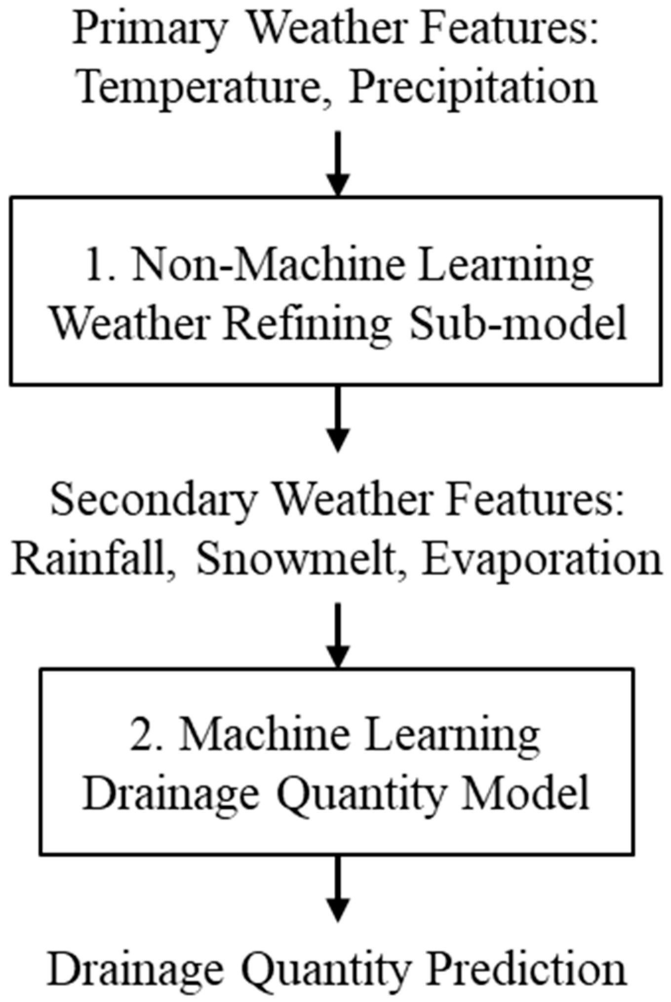
2. Methodology
2.1. Weather Refining Sub-Model
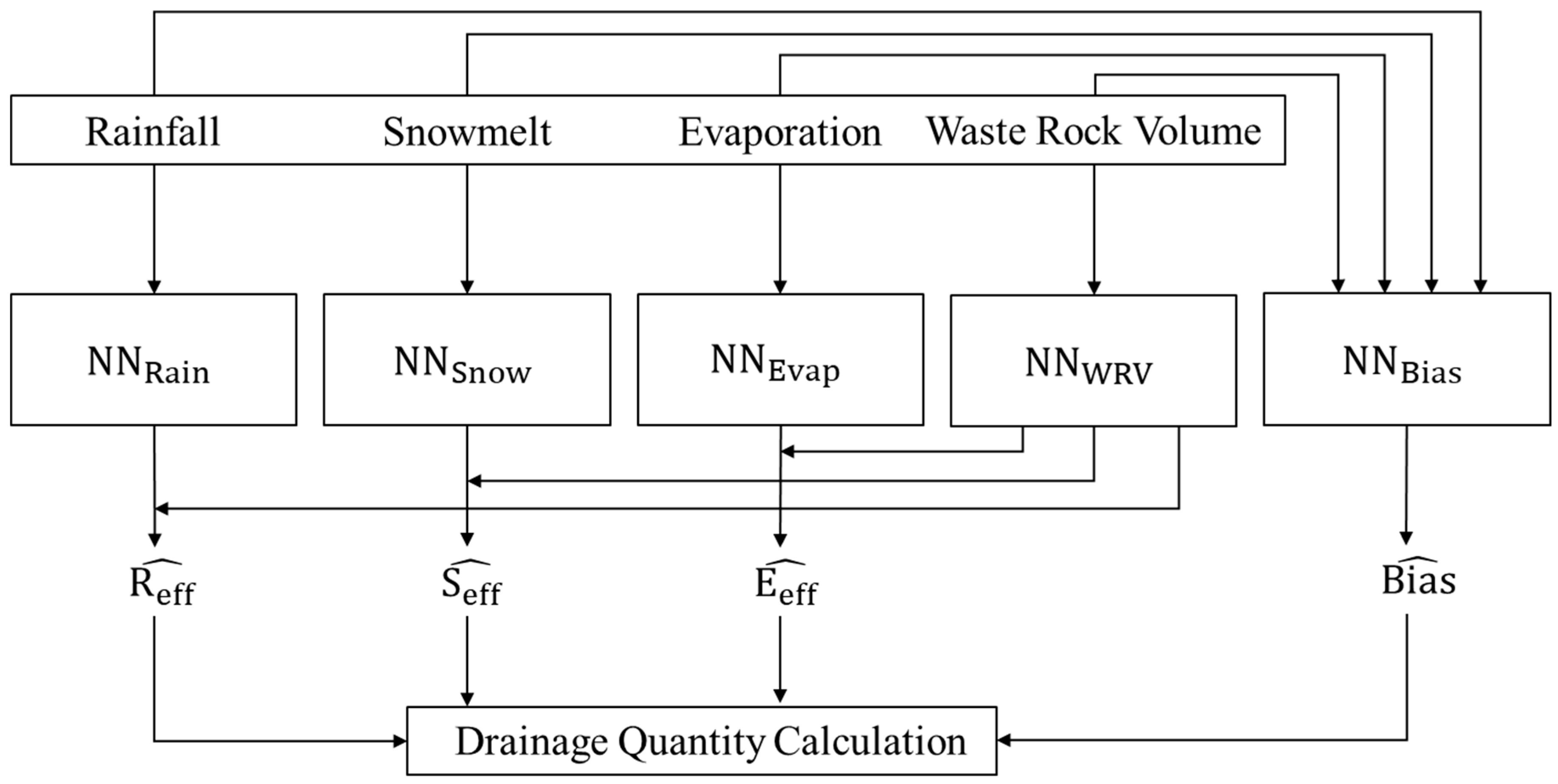
2.2. Machine Learning Drainage Quantity Model
2.2.1. Conceptual Model
2.2.2. Neural Network Architecture Design
2.2.3. Loss Function Design
2.2.4. Model Tuning
3. Results and Discussion
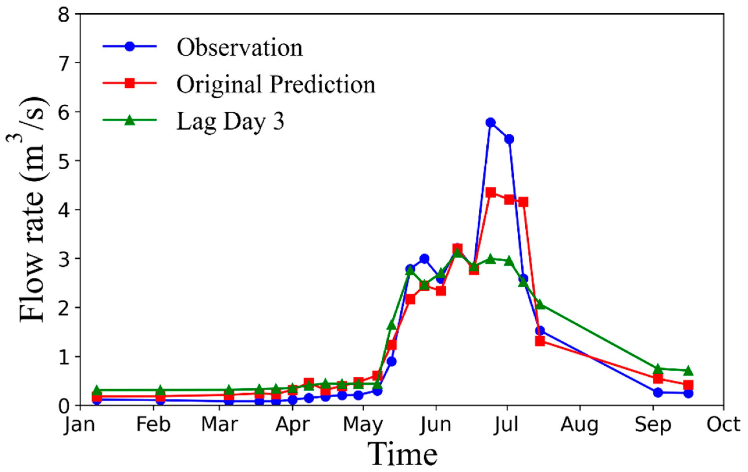
3.1. Model Training and Testing
3.2. Sensitivity Tests
3.3. Verification of the Non-Negative Correlations by Monotonicity Test
3.4. The Impact of Current Weather Conditions on Future Drainage Quantities
4. Conclusions
Author Contributions
Funding
Data Availability Statement
Conflicts of Interest
References
- Wolkersdorfer, C.; Nordstrom, D.K.; Beckie, R.D.; Cicerone, D.S.; Elliot, T.; Edraki, M.; Valente, T.; França, S.C.A.; Kumar, P.; Lucero, R.A.O.; et al. Guidance for the integrated use of hydrological, geochemical, and isotopic tools in mining operations. Mine Water Environ. 2020, 39, 204–228. [Google Scholar] [CrossRef]
- Tremblay, G.A.; Hogan, C.M. (Eds.) Mine Environment Neutral Drainage (MEND) Manual 5.4.2d: Prevention and Control; Canada Centre for Mineral and Energy Technology: Ottawa, ON, Canada, 2001; Available online: http://mend-nedem.org/wp-content/uploads/5-4-2dVolume4_PreventionControlL.pdf (accessed on 17 August 2023).
- Lefebvre, R.; Hockley, D.; Smolensky, J.; Geélinas, P. Multiphase Transfer Processes in Waste Rock Piles Producing Acid Mine Drainage: 1: Conceptual Model and System Characterization. J. Contam. Hydrol. 2001, 52, 137–164. [Google Scholar] [CrossRef]
- Nichol, C.F. Transient Flow and Transport in Unsaturated Heterogeneous Media: Field Experiments in Mine Waste Rock; The University of British Columbia: Vancouver, BC, Canada, 2002. [Google Scholar]
- Nichol, C.; Smith, L.; Beckie, R. Field-Scale Experiments of Unsaturated Flow and Solute Transport in a Heterogeneous Porous Medium. Water Resour. Res. 2005, 41, W05018. [Google Scholar] [CrossRef]
- Brusseau, M.L.; Rao, P.S.C. Modeling Solute Transport in Structured Soils: A Review. Geoderma 1990, 46, 169–192. [Google Scholar] [CrossRef]
- Flury, M.; Yates, M.V.; Jury, W.A. Numerical analysis of the effect of the lower boundary condition on solute transport in lysimeters. Soil Sci. Soc. Am. J. 1999, 63, 1493–1499. [Google Scholar] [CrossRef]
- Smith, L.; López, D.; Beckie, R. Hydrogeology of Waste Rock Dumps; Victoria, B.C., Ed.; British Columbia Ministry of Energy, Mines and Petroleum Resources: Cranbrook, BC, Canada; CANMET: Ottawa, ON, Canada, 1995. [Google Scholar]
- Gélinas, P.; Lefebvre, R.; Choquette, M. Monitoring of Acid Mine Drainage in a Waste Rock Dump. In Proceedings of the Secondary International Conference on Environmental Issue and Management of Waste in Energy and Mineral Production, Calgary, AB, Canada, 1–4 September 1992; Volume 6, pp. 747–757. [Google Scholar]
- Ramasamy, M.; Power, C.; Mkandawire, M. Numerical Prediction of the Long-term Evolution of Acid Mine Drainage at a Waste Rock Pile Site Remediated with an HDPE-lined Cover System. J. Contam. Hydrol. 2018, 216, 10–26. [Google Scholar] [CrossRef]
- King, M. Groundwater and contaminant transport modelling at the sydney tar ponds. In Proceedings of the 56th Annual Canadian Geotechnical Conference and 4th Joint IAH-CNC/CGS Groundwater Specialty Conference, Winnipeg, MB, Canada, 28 September–1 October 2003; pp. 10–26. [Google Scholar]
- Hendrickx, J.M.H.; Flury, M. Uniform and Preferential Flow Mechanisms in the Vadose Zone. In Conceptual Models of Flow and Transport in the Fractured Vadose Zone; The National Academies Press: Washington, DC, USA, 2001; pp. 149–187. [Google Scholar]
- Pedretti, D.; Mayer, K.U.; Beckie, R.D. Stochastic Multicomponent Reactive Transport Analysis of Low Quality Drainage Release from Waste Rock Piles: Controls of the Spatial Distribution of Acid Generating and Neutralizing Minerals. J. Contam. Hydrol. 2017, 201, 30–38. [Google Scholar] [CrossRef]
- Pedretti, D.; Vriens, B.; Skierszkan, E.K.; Baják, P.; Mayer, K.U.; Beckie, R.D. Evaluating Dual-Domain Models For Upscaling Multicomponent Reactive Transport in Mine Waste Rock. J. Contam. Hydrol. 2022, 244, 103931. [Google Scholar] [CrossRef]
- Pedretti, D.; Mayer, K.U.; Beckie, R.D. Controls of Uncertainty in Acid Rock Drainage Predictions from Waste Rock Piles Examined through Monte-Carlo Multicomponent Reactive Transport. Stoch. Environ. Res. Risk Assess. 2020, 34, 219–233. [Google Scholar] [CrossRef]
- Smith, L.; Beckie, R. Hydrologic and Geochemical Transport Processes in Mine Waste Rock. In Environmental Aspects of Mine Wastes; Mineralogical Association of Canada: Haywood County, NC, USA, 2003; Volume 31. [Google Scholar]
- Jiang, C.; Zhu, S.; Hu, H.; An, S.; Su, W.; Chen, X.; Li, C.; Zheng, L. Deep Learning Model Based on Big Data for Water Source Discrimination in an Underground Multiaquifer Coal Mine. Bull. Eng. Geol. Environ. 2022, 81, 26. [Google Scholar] [CrossRef]
- Ma, L.; Huang, C.; Liu, Z.S.; Morin, K.A.; Aziz, M.; Meints, C. Artificial Neural Network for Prediction of Full-scale Seepage Flow Rate at the Equity Silver Mine. Water. Air. Soil Pollut. 2020, 231, 179. [Google Scholar] [CrossRef]
- Zhang, C.; Ma, L.; Liu, W. A machine learning approach for prediction of the quantity of mine waste rock drainage in areas with spring freshet. Minerals 2023, 13, 376. [Google Scholar] [CrossRef]
- Karniadakis, G.E.; Kevrekidis, I.G.; Lu, L.; Perdikaris, P.; Wang, S.; Yang, L. Physics-Informed Machine Learning. Nat. Rev. Phys. 2021, 3, 422–440. [Google Scholar] [CrossRef]
- Tartakovsky, A.M.; Marrero, C.O.; Perdikaris, P.; Tartakovsky, G.D.; Barajas-Solano, D. Physics-informed deep neural networks for learning parameters and constitutive relationships in subsurface flow problems. Water Resour. Res. 2020, 56, e2019WR026731. [Google Scholar] [CrossRef]
- Huschke, R.E. Glossary of meteorology. Weatherwise 1960, 13, 69–86. [Google Scholar] [CrossRef]
- Kittel, C.; Kroemer, H.; Scott, H.L. Thermal Physics, 2nd ed. Am. J. Phys. 1998, 66, 164–167. [Google Scholar] [CrossRef]
- Laramie, R.L.; Schaake, J.C. Simulation of the Continuous Snowmelt Process; Cambridge Ralph, M., Ed.; Parsons Laboratory for Water Resources and Hydrodynamics, Massachusetts Institute of Technology: Cambridge, MA, USA, 1972; Available online: https://hdl.handle.net/1721.1/142971 (accessed on 3 July 2024).
- van der Knijff, J.M.; Younis, J.; de Roo, A.P.J. LISFLOOD: A GIS-Based Distributed Model for River Basin Scale Water Balance and Flood Simulation. Int J Geogr Inf Sci. 2010, 24, 189–212. [Google Scholar] [CrossRef]
- Allen, R.G.; Pereira, L.S.; Raes, D.; Smith, M. Crop Evapotranspiration—Guidelines for Computing Crop Water Requirements—FAO Irrigation and Drainage Paper 56; FAO: Rome, Italy, 1998; Available online: https://www.fao.org/4/x0490e/x0490e00.htm (accessed on 3 July 2024).
- Wang, T.; Hamann, A.; Spittlehouse, D.; Carroll, C. Locally Downscaled and Spatially Customizable Climate Data for Historical and Future Periods for North America. PLoS ONE 2016, 11, e0156720. [Google Scholar] [CrossRef] [PubMed]
- Ma, L.; Huang, C.; Liu, Z.S.; Morin, K.A.; Aziz, M.; Meints, C. The Correlation between Drainage Chemistry and Weather for Full-Scale Waste Rock Piles Based on Artificial Neural Network. J. Contam. Hydrol. 2021, 239, 103793. [Google Scholar] [CrossRef] [PubMed]
- Cho, K.; van Merriënboer, B.; Bahdanau, D.; Bengio, Y. On the Properties of Neural Machine Translation: Encoder–decoder Approaches. In Proceedings of the SSST 2014—8th Workshop on Syntax, Semantics and Structure in Statistical Translation, Doha, Qatar, 25 October 2014. [Google Scholar] [CrossRef]
- Bergstra, J.; Yamins, D.; Cox, D.D. Making a Science of Model Search: Hyperparameter Optimization in Hundreds of Dimensions for Vision Architectures. In Proceedings of the 30th International Conference on Machine Learning, ICML 2013, Atlanta, GA, USA, 16–21 June 2013. [Google Scholar]
- Kingma, D.P.; Ba, J.L. Adam: A Method for Stochastic Optimization. In Proceedings of the 3rd International Conference on Learning Representations, ICLR 2015—Conference Track Proceedings, San Diego, CA, USA, 7–9 May 2015. [Google Scholar]


| Units | Learning Rate | λp | λr | |
|---|---|---|---|---|
| Station 1 | 14 | 0.0005 | 1.5 | 1 |
| Station 2 | 32 | 0.0005 | 1.5 | 0.1 |
| Station 3 | 8 | 0.0005 | 1.5 | 0.1 |
| Distance (km) | Elevation Differences (m) | |
|---|---|---|
| Station 1 | 49.0 | 1060 |
| Station 2 | 49.2 | 1060 |
| Station 3 | 5.0 | 660 |
| 1RMSE (m3/s) | 2RMSE (m3/s) | 2NSE | ||||
|---|---|---|---|---|---|---|
| Train | Test | Train | Test | Train | Test | |
| Station 1 | 0.4449 | 0.9175 | 0.5330 | 0.5701 | 0.8052 | 0.8904 |
| Station 2 | 0.9033 | 1.0108 | 0.4920 | 0.5660 | 0.9244 | 0.9082 |
| Station 3 | 0.2545 | 0.4400 | 0.4387 | 0.3985 | 0.8426 | 0.8616 |
Disclaimer/Publisher’s Note: The statements, opinions and data contained in all publications are solely those of the individual author(s) and contributor(s) and not of MDPI and/or the editor(s). MDPI and/or the editor(s) disclaim responsibility for any injury to people or property resulting from any ideas, methods, instructions or products referred to in the content. |
© 2025 by the authors. Licensee MDPI, Basel, Switzerland. This article is an open access article distributed under the terms and conditions of the Creative Commons Attribution (CC BY) license (https://creativecommons.org/licenses/by/4.0/).
Share and Cite
Zhang, C.; Ma, L.; Liu, W. Prediction of Mine Waste Rock Drainage Quantity Using a Machine Learning Model with Physical Constraints. Minerals 2025, 15, 194. https://doi.org/10.3390/min15020194
Zhang C, Ma L, Liu W. Prediction of Mine Waste Rock Drainage Quantity Using a Machine Learning Model with Physical Constraints. Minerals. 2025; 15(2):194. https://doi.org/10.3390/min15020194
Chicago/Turabian StyleZhang, Can, Liang Ma, and Wenying Liu. 2025. "Prediction of Mine Waste Rock Drainage Quantity Using a Machine Learning Model with Physical Constraints" Minerals 15, no. 2: 194. https://doi.org/10.3390/min15020194
APA StyleZhang, C., Ma, L., & Liu, W. (2025). Prediction of Mine Waste Rock Drainage Quantity Using a Machine Learning Model with Physical Constraints. Minerals, 15(2), 194. https://doi.org/10.3390/min15020194