Article

Geoscientific Input Feature Selection for CNN-Driven Mineral Prospectivity Mapping

1
Department of Physics, University of Toronto, 60 St. George Street, Toronto, ON M5S 1A7, Canada
2
Department of Earth Sciences, University of Toronto, 22 Ursula Franklin Street, Toronto, ON M5S 3B1, Canada
*
Author to whom correspondence should be addressed.
Minerals 2025, 15(12), 1237; https://doi.org/10.3390/min15121237 (registering DOI)
Submission received: 6 October 2025 / Revised: 16 November 2025 / Accepted: 21 November 2025 / Published: 23 November 2025
(This article belongs to the Special Issue Feature Papers in Mineral Exploration Methods and Applications 2025)

Abstract

In recent years, machine learning techniques such as convolutional neural networks have been used for mineral prospectivity mapping. Since a diverse range of geoscientific data is often available for training, it is computationally challenging to select a subset of features that optimizes model performance. Our study aims to demonstrate the effect of optimal input feature selection on convolutional neural network model performance in mineral prospectivity mapping applications. We demonstrate results from both exhaustive and algorithmic feature selection methods in the context of copper porphyry prospectivity modeling and analyze the performance and stability of optimally trained models. Using the QUEST dataset from central interior British Columbia, such a feature selection technique improves model performance by 6.8% over models that use all available features, yet consumes around 2.2% of the computational resources needed to exhaustively search for the optimal feature subset.

1. Introduction

Mineral prospectivity mapping (MPM) is a systematic approach used to assess the potential occurrence of mineral deposits in a geographic area. It involves the integration of geoscientific information such as geological, geochemical, geophysical, and remote sensing data to create predictive models that identify favorable areas for mineral exploration. The primary objective of MPM is to guide efficient and cost-effective exploration strategies, focusing activities on areas with the highest probability of success while minimizing costs and reducing environmental impact. Classic efforts in MPM consist of empirical data integration through expert knowledge [1]. However, recent advancements in the computational sciences, particularly machine learning (ML), have allowed for a high degree of data integration and extraction for classification tasks.
Supervised techniques such as decision trees [2], random forest [3], and Support Vector Machines (SVMs) [4] are widely used for MPM, but such methods do not take spatial relationships into account directly. However, mineral deposits and their respective geoscientific signatures are highly spatially correlated, and accounting for such relationships is relevant for MPM. One supervised machine learning model that accounts for spatial correlations is a Convolutional Neural Network (CNN). In recent years, a diverse range of CNN-based techniques have been used for MPM problems [5,6,7]. However, one of the crucial steps in all forms of MPM is the appropriate and optimal selection of data in relation to the mineral deposit of interest. Various sets of geoscientific data categories are deemed optimal for different exploration targets and corresponding mineral systems [3,5]. Most CNN-based MPM workflows do not involve optimal input feature selection and use all abundantly available feature categories [5], with only a small subset of MPM workflows using non-exclusionary feature importance assignments through attention-based approaches, where a model learns the optimal importance of each training feature for individual labels [7]. One could argue that, in principle, active input selection is unnecessary given the appropriate choice of model architecture and hyperparameters, as the network will automatically learn to allocate lower weights (i.e., importance) to data categories that contribute to suboptimal classification, especially if input feature importance (e.g., attention-based algorithms) is implemented in the learning algorithm. However, embedded techniques such as attention-based learning have several disadvantages. Examples include the non-exclusionary weighting of features, the non-unique relationship between attention weights and performance, and limited explainability. On the other hand, differences in the geographical scale across different input features can be problematic during the learning process, especially in cases where data is interpolated. For these reasons, we seek to understand how an exclusionary selection of input features affects CNN-based MPM models and how these effects can be interpreted.
A simple and motivating example of the importance of input feature selection can be given through the binary classification of dog and cat images. A successful and widely implemented CNN architecture is AlexNet [8], which accepts images in RGB format, as a collection of three separate color input layers. We train an AlexNet model on dog images, together with four altered and unaltered versions of cat images [9]: standard cat images, cat images with a noisy green layer, cat images in which the green layer is replaced by that of a random dog, and cat images with the green layer fully removed. All network hyperparameters, as well as the number of training epochs, remain fixed. Figure 1 demonstrates examples of a cat image under each alteration category as well as the corresponding model validation accuracy.
The performance of the AlexNet CNN architecture in these four scenarios shows that even as little as 8.5% noise can reduce model validation accuracy by more than 30%, while adding a completely uncorrelated color layer to the RGB images reduces the model to a random classifier. On the other hand, removing the altered layer produces better validation accuracy, though subpar compared to models trained on the unaltered data. This case represents a very simple evaluation and selection process, in which only three or fewer layers of data are used. In most MPM cases, tens of geoscientific features are often used as input features, where one or more input features could significantly degrade validation performance. This can be caused by inherently high levels of uncertainty in certain types of geoscientific data (e.g., geological boundary delineations); or a lack of strong correlation of some data types to the mineral system of interest (e.g., mismatch in the apparent depth scales of surveys and that of the mineral system). This simple example motivates a corresponding study for input feature selection in CNN-driven MPM.
The selection of the most appropriate subset of features is effectively an optimization problem. In its most basic form, the preferred set of data can be discretely broken down further, with each subset being exhaustively evaluated [10]. Other more statistically sophisticated methods include using pairwise correlations of input features to reduce the cardinality of the feature space [11], embedding a Lasso and L 2 -norm penalty in the neural network’s loss function to ensure small weight (i.e., weights related to features with weak predictive potential) are zeroed after training [12], or more novel methods such as Global Sensitivity Analysis (GSA) [13].
Most models in MPM studies train on the full set of presumed predictive features, spanning geological, geochemical, and geophysical layers. To assess input feature influence, these studies often compute post hoc feature importance after training and validating on occurrence labels, often to satisfy AI explainability aims [14,15,16,17,18]. However, these analyses usually stop short of operationalizing their findings, with only a few studies explicitly incorporating wrapper input feature selection or feature selection and re-training in MPM, through decision tree-based methods such as random forest [19,20]. In other words, they do not prune the input feature set and re-fit the model, so the asserted importance ranking is never stress-tested.
Redundant layers remain in the stack and, even if assigned low importance, can exert residual influence through correlation structure or regularization paths, which is particularly consequential in sparsely labeled regions where inference is purely extrapolative. Moreover, input feature importance is typically estimated while all features are present simultaneously, so multicollinearity and spatial autocorrelation induce implicit dependencies among evidence layers learned by the model, which can limit the practical explainability of the prospectivity model. Without a formal selection-and-refit step (e.g., wrapper-based subset search), practitioners cannot quantify whether an evidence stack would deliver equal or better discrimination, improved calibration, and reduced variance, nor can they provide reliable guidance on which layers are worth acquiring or preprocessing.
In this study, we aim to demonstrate the impact of categorical input feature selection on the performance and stability of CNN-based MPM. To provide a simple benchmark workflow, we run an exhaustive search for the best input data as well as a simple, yet effective alternative selection technique called Multi-armed Bandit (MAB) to further illustrate the effect of input feature selection on CNN-based MPM, with the objective of improving copper porphyry prospectivity mapping of central interior British Columbia, Canada.

2. Methodology

2.1. Data and CNN Model

In this study, we use data from the QUEST project for copper porphyry prospectivity mapping. The QUEST project is an extensive data collection campaign, which includes geological, geochemical, and geophysical surveys designed to attract the mineral exploration industry to an under-explored region of British Columbia between Williams Lake and Mackenzie [21]; data from the acquisition program have been used for MPM of central British Columbia in recent years [5,22,23]. The QUEST project is focused on the Quesnel Terrane, which has a number of known copper and gold porphyry occurrences.
The QUEST data can be broken down into geological, geochemical, and geophysical categories. The geological category consists of the distance to the closest fault, binary indicators for 5 geological bedrock classes (e.g., intrusive, metamorphic, sedimentary, ultramafic, and volcanic rocks), 55 geological bedrock subclasses (e.g., alkaline volcanic rocks, limestone, meta-sediments), and the minimum/maximum geological ages. The geochemical category consists of trace quantity data of 42 elements (e.g., Au, Ni, Pb). Lastly, the geophysical category consists of 5 gravity products, 5 magnetics products, and 7 channels of Versatile Time Domain Electromagnetics (VTEM) data (a total of 17 geophysical input features).
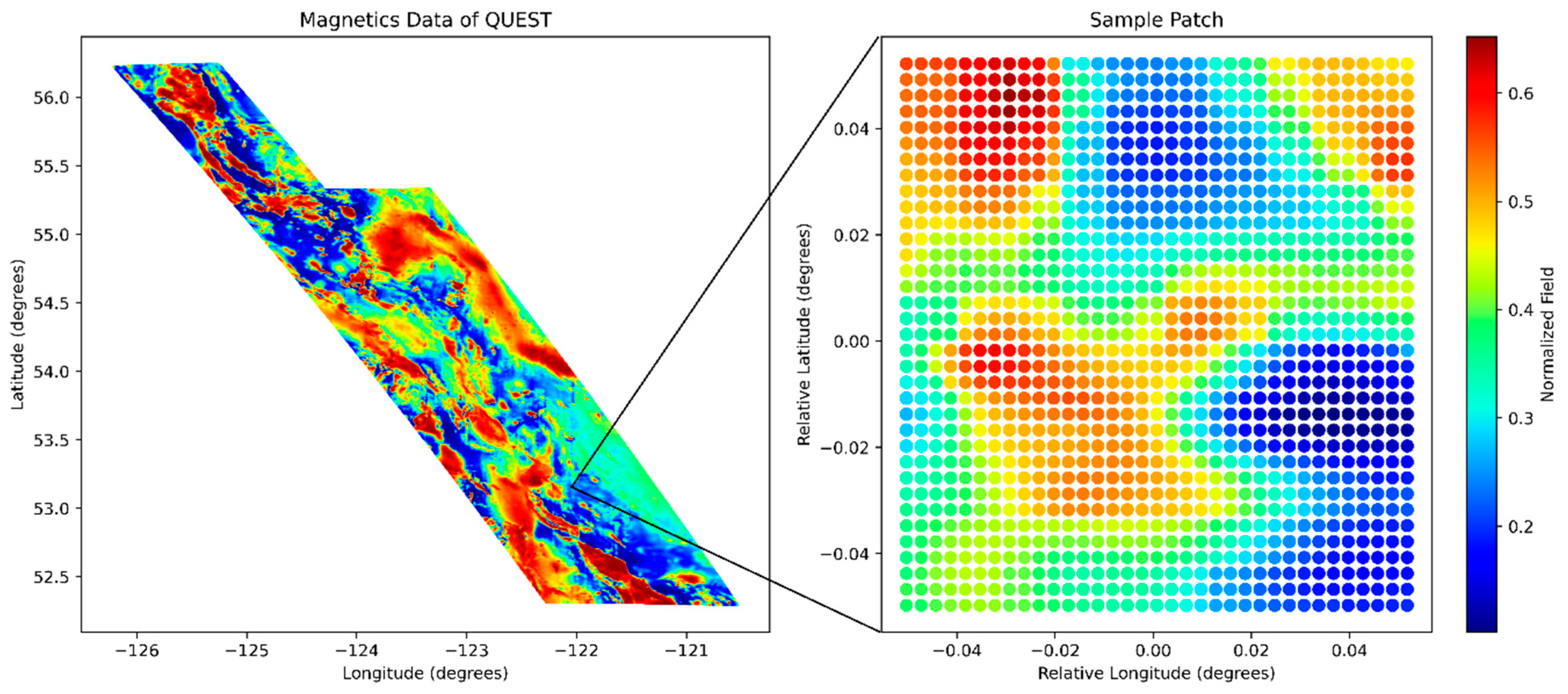
In the case of our MPM problem, the input is a so-called data cube, which is a collection of 2D geoscientific data, mentioned above (i.e., [spatial information, geoscientific data]). The entire geographic area of interest is cropped into 572,212 patches (i.e., sub-cubes of the entire data cube), with an extent of [0.114 degrees North × 0.114 degrees East] (note that these patches are allowed to geographically overlap). In addition, the training, validation, and inference stages use 1950 randomly sampled data sub-cubes each, with an evenly split class label balance. The magnetics data, together with a sample crop, are provided as an example for an individual layer of the data cube in Figure 2.
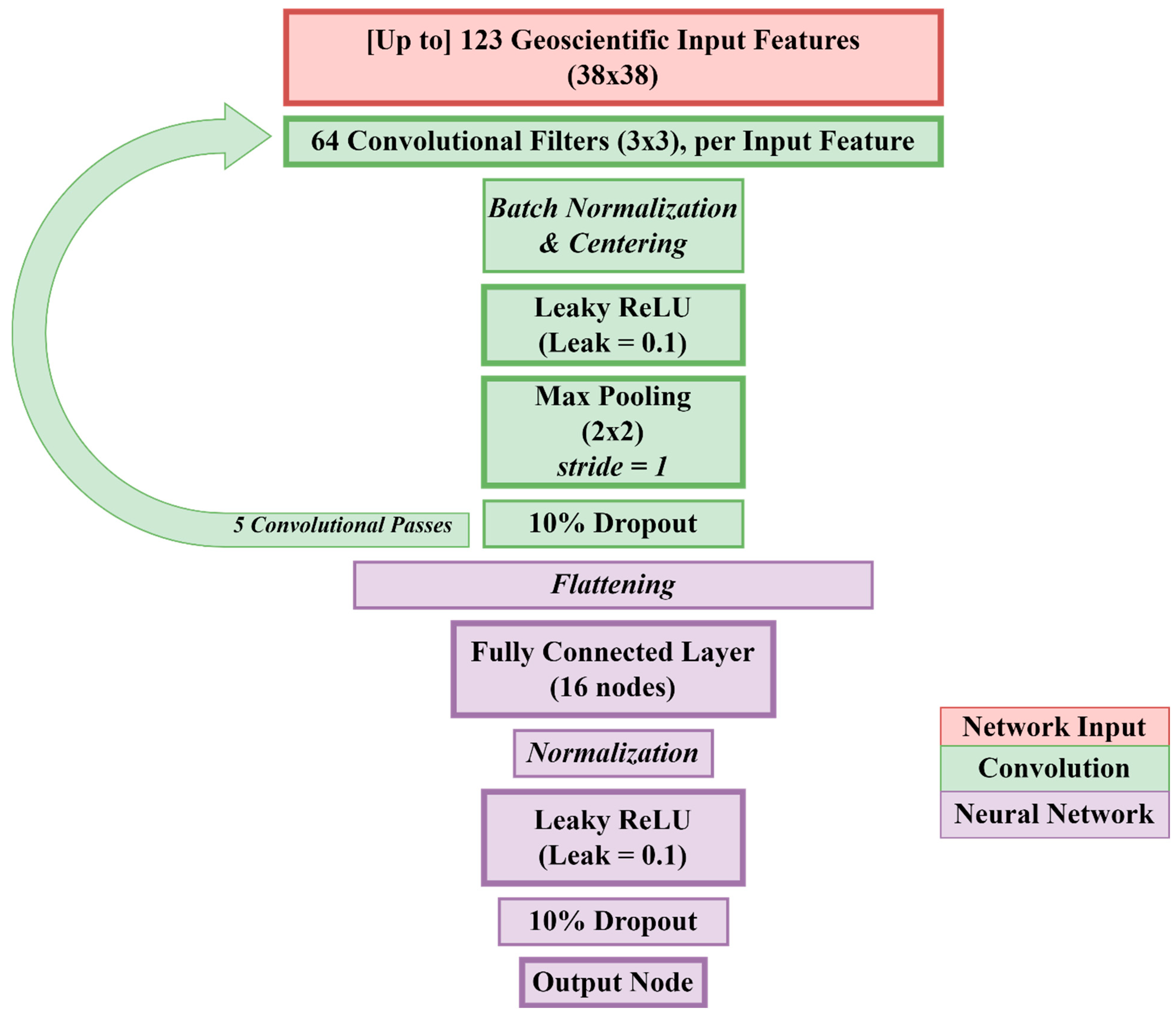
The labels of the patches in the training and validation set are assigned by their containment of mineral occurrences, as well as the position of the deposit relative to the frame of the patch. We defined a labeling criterion, where a geographic patch is assigned a positive label if a mineral occurrence falls within a fourth crop size distance of the patch center. Those patches that have mineral occurrences within a 10 km distance outside of that region are labeled as interim patches. Note that these interim batches represent the uncertainty in label assignment and are not used for training or validation of CNN models. The rest of the possible patches are assigned a negative label. In addition, the hyperparameters of our CNN model are manually tuned and optimized for the MPM task, and fixed throughout the study. A list of our CNN hyperparameters is provided in Appendix A, Table A1, for reference. The CNN models are trained on the labels south of 53.2 degrees and validated on the labels north of 54.7 degrees. Model predictions are made in the central region between these latitudes (see Figure 3 for the architecture of the CNN).

2.2. Optimal Input Feature Selection

2.2.1. Optimization Metric

In this study, the optimization metric is designed such that it reflects the overall goodness of a prospectivity model. A good prospectivity model is one that makes the most true positive predictions, while making the fewest false positive predictions. The consequences of false positive predictions can have detrimental financial implications for any exploration effort, leading to misallocation of resources. An effective tool to numerically frame this objective is through a Receiver Operating Characteristic (ROC), which is a curve describing the relationship between the rate of true positive predictions (TPR) and the rate of false positive predictions (FPR) as a function of a classification threshold p t h r . These ratios can be calculated by Equations (1) and (2), as follows:
T P R = T P T P + F N
F P R = F P F P + T N
where TP, TN, FN, and FP are the counts of true positive, true negative, false negative, and false positive predictions, respectively. Notice that for a determined predictive model and prediction threshold p t h r , TPR and FPR are independent of prediction class imbalance.
The ROC curve can be plotted for any four elements in the confusion matrix. However, it should be noted that the negative mineral occurrence labels are less certain than positive mineral occurrence labels in large-scale MPM. This is due to the lack of confirmed negative occurrence labels in the QUEST dataset. Negative labels are either assigned based on some distance criterion or geological assumptions. This leads to less robust validation on negative labels.
A regression model is chosen for the CNN (i.e., returning scores that range from 0 to 1), and can be validated if a threshold value p t h r   is defined, with regression scored above p t h r validated as a positive prediction and negative otherwise (in this work, p t h r = 0.5). We define a metric to unify the notion of maximizing the rate of true positive predictions and minimizing the rate of false positive predictions of the prospectivity model (Equation (3))
R = 1 ( 1 T P R ) 2 + ( F P R ) 2 d m a x 2 ,   d m a x = 2 .
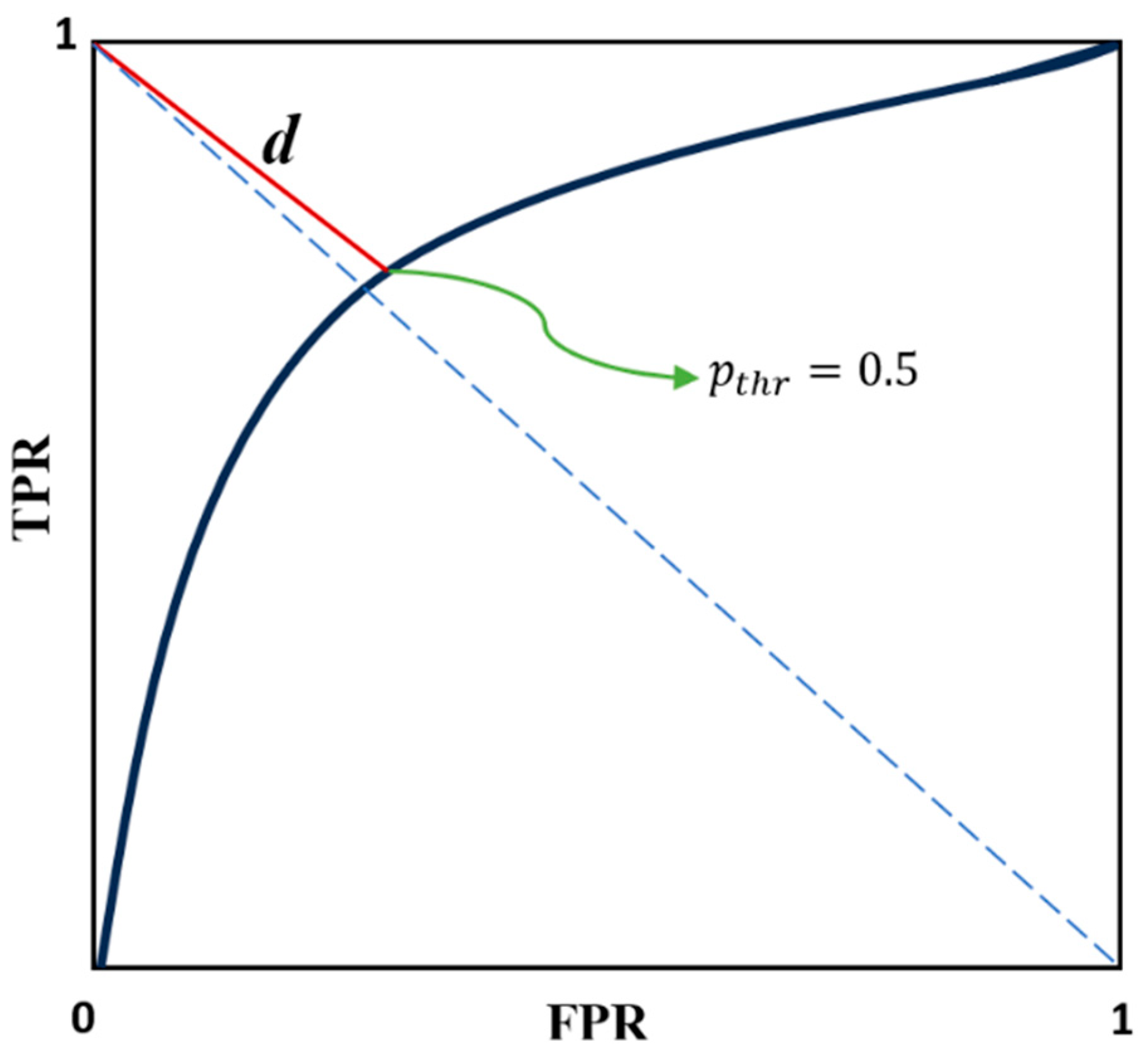
where R represents an adjusted Euclidean distance from (FPR, TPR) = (0, 1) to the (FPR, TPR), corresponding to p t h r = 0.5 (R = 1 indicates a perfect predictor). This reward formulation encourages the selection of models that produce a high true positive prediction rate while simultaneously having a low false positive prediction rate.
Unlike other validation metrics such as the F1 score and Matthews Correlation Coefficient, the reward metric R is not affected by label class imbalance, since the expressions for TPR and FPR rates involve one class in each instance. A visual rationale for this choice of reward is also shown in Figure 4. This metric is used to represent model performance throughout the rest of this study. Note that this optimization metric is different from the loss of the CNN model. The calculated loss of the CNN model incorporates false and true predictions for both positive and negative validation labels, whereas the optimization metric R only incorporates false positive and true positive predictions (e.g., a model can have a very high rate of false negative predictions and still obtain a high R score, given its false positive prediction rate is minimal).

2.2.2. Exhaustive Search

An exhaustive search of all possible training feature subsets is performed over geological class, geological subclass, minimum/maximum geological age, distance to nearest fault, geochemical data, gravity, magnetics, and VTEM data to create a benchmark for optimization efficiency. According to the breakdown in Table 1, there are 255 possible combinations to investigate. The categories in Table 1 can be further broken down to allow for more input feature combinations, as many categories encompass multiple sub-features, particularly geochemistry. However, this raises the number of configurations up to a count of 10 37 , and presents little practical benefit compared to the said associated growth in the search space.
Since stochasticity is central to the machinery of CNNs (mainly due to stochastic gradient descent, dropout, and stochastic network weight initializations) [24], the model performance for a particular training feature subset cannot be evaluated from a single CNN run (i.e., complete training and validation operations) of the CNN algorithm, and the result of multiple CNN runs are needed for calculating statistically significant performance figures. Thus, the number of independent training and validations (i.e., N r u n ) need to be high (180 CNN runs for each input feature configuration).

2.2.3. Multi-Armed Bandits

The Multi-armed Bandit (MAB) gets its name from the idea of a gambler who wishes to maximize their total winnings over time, given a row of slot machines (often called one-armed-bandits). In MAB problems, a decision-making agent is faced with a set of actions (i.e., the “arms” of the MAB), and must decide which action to select at each step with the goal of maximizing its total cumulative reward (see Equation (3)) [25]. MAB algorithms efficiently allocate limited resources (in this case, computing power and time) by balancing exploration (i.e., taking a random action) and exploitation (i.e., taking the perceived optimal action at the time), and are used to optimize decision-making in dynamic and uncertain environments. Examples range from infill drilling in mining [26] to recommendation systems [27] and portfolio management in finance [28].
The action is defined as a tuple, containing the chosen data within each geoscientific data category (see Section 3.1). The MAB has a “lever” for each possible data subset derived by Table 1, and each can be pulled independently. In this case, pulling a lever is equivalent to training the CNN model on the chosen input feature subset and observing the validation performance of the model.
An action–value method is applied to numerically relate the concepts of action to reward. The premise of action–value functions is the determination of an action’s value with respect to prior experiences. A simple action–value function is defined as the average rewards of previous instances:
Q n a =   i = 1 n R i ( a ) n
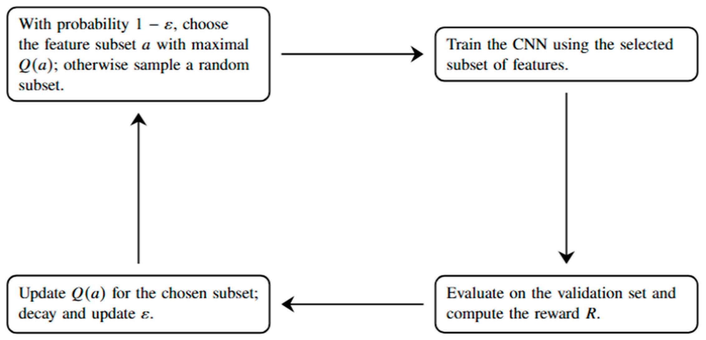
where Q n a   is the average value of action a after taking it n times; and R i is the reward received after the i t h choice of action a (see Equation (3)). The action associated with the maximum Q value (i.e., Q m a x calculated by Equation (4)) is considered the most optimal action until that point, which would be exploited by the agent to maximize future rewards. Figure 5 demonstrates how the MAB algorithm is integrated with the CNN training and validation process.
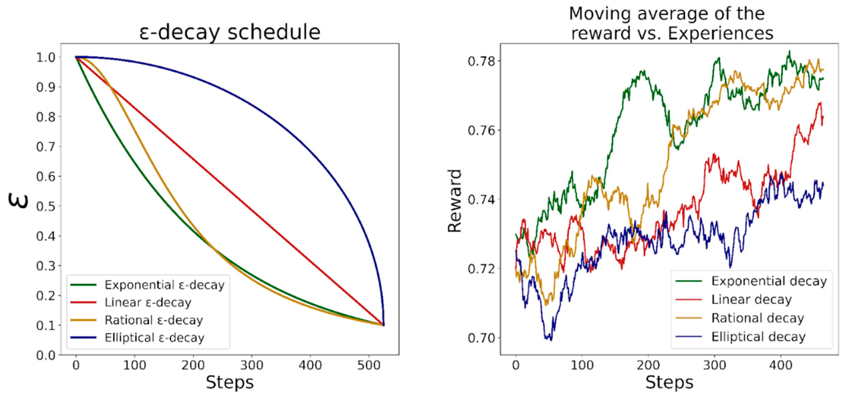
MAB agents cannot simply exploit an action they currently believe to be optimal, they must also explore other potentially optimal actions. The trade-off between exploration and exploitation can be managed through a simple and widely used algorithm called Ɛ-greedy. In this method, the agent exploits its experience by taking the action associated with Q m a x with a 1 − Ɛ probability (randomly breaking ties if multiple actions are believed to be equally optimal), and explores by taking a random action with a probability Ɛ. The conventional Ɛ-greedy strategy is modified to let the agent explore a wide range of actions at early MAB steps, and gradually become exploitative as it gains experience. This can be performed by decaying the value of Ɛ over MAB steps in several ways. Overall, four ε-decay schedules are initially tested, namely linear, exponential, rational, and elliptical decays (see Appendix A, Table A2). The decay rate is set such that epsilon reaches 0.1 at the 1000th step, at which point a r g m a x [ Q a ] is the result of the optimization process.

3. Optimized Mineral Prospectivity Results

3.1. Exhaustive Search for Optimal Input

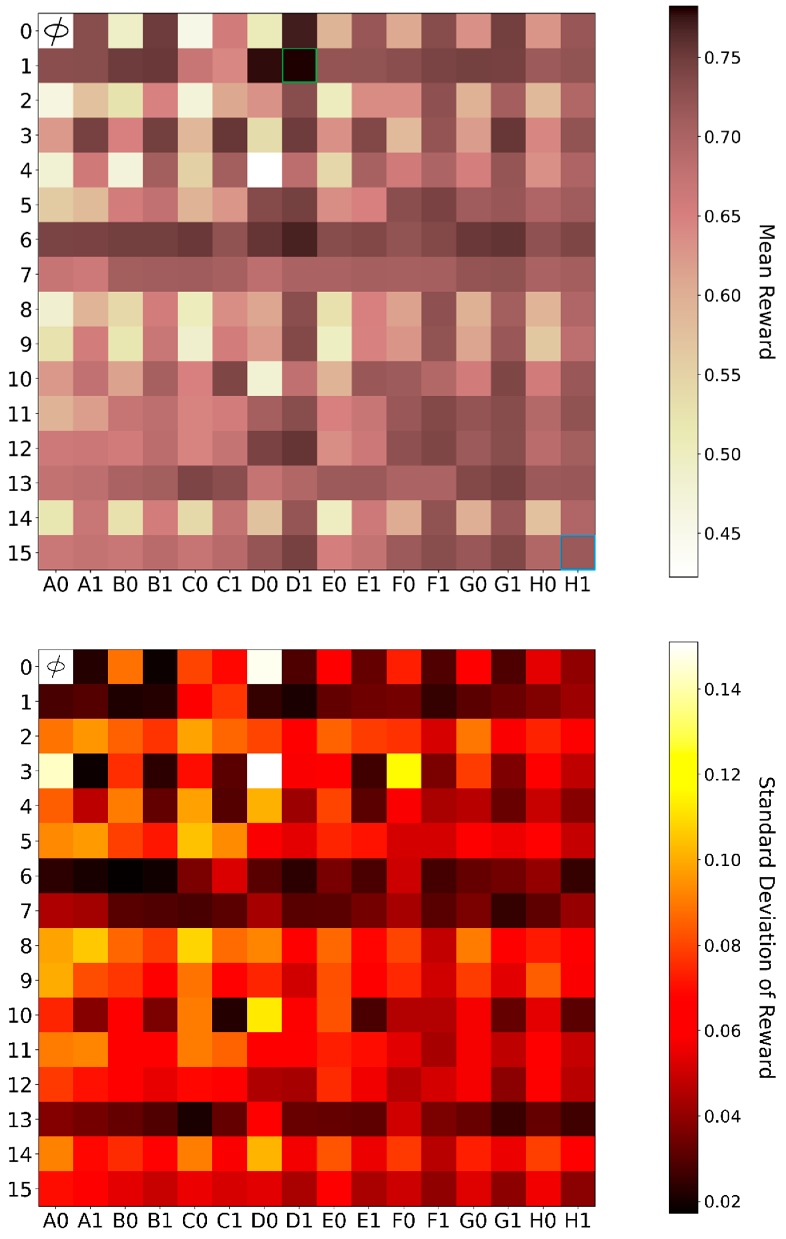
The exhaustive search concludes that the best training input feature subset is geological class, geochemical, and VTEM data (See Table 1 and Figure 6). This implies that the optimal set of input features consists of 53 individual layers (i.e., 2D rasters) as opposed to 123 individual layers for the entire available dataset. The expected reward for the full inclusion of all feature categories in an expected reward of 0.714 ± 0.038, and training on the optimal input feature set produces an expected reward of 0.782 ± 0.021, which is a statistically significant improvement.
Note that the spatial training and validation split, as well as the choice of hyperparameters, weight initialization, and classification threshold, remain fixed for individual input feature configurations (see Table A1). Therefore, other than the choice of training feature subset, the variability in validation performance across different feature subsets is mainly due to the stochasticity in the learning process of the CNN (e.g., node dropout in the neural network). Other commonly examined factors include noise, feature collinearity, and data leakage; however, they are inherently related to the input training features.
The completion of such a number of CNN model trainings and validations necessitates the use of high-performance computing (HPCs with NVIDIA A100SXM4 GPUs), taking a total of 3364 GPU hours (in addition, note that the batch configuration is fixed and equal to 32 crops throughout this study). In addition, any further breakdown of data can drastically increase the number of needed trainings and validations. These challenges motivate the use and incorporation of alternative data selection techniques, such as an MAB.

3.2. MAB Search for Optimal Input

For our Ɛ-greedy strategy, the rational and exponential decay types display roughly even performance, and are superior to the other decay schedules (see Figure 7). The exponential decay schedule is used for the rest of this study.
The MAB agent concluded that using geological class and, VTEM together with geochemistry is the most optimal set of training features for the CNN-based MPM, which agrees with the exhaustive search (note that MAB results were consistent over five separate iterations of the MAB algorithm). In addition, this result is fully consistent for several runs of the MAB algorithm. Using this choice of geoscientific training features, we obtain an average model reward of more than 78.2%, which is a 6.8% improvement over training on all features (see Figure 6 and Figure 8). This result is particularly significant considering that most configuration performance distributions are heavily overlapped, usually within a tenth of their standard deviation. This implies that the MAB technique can handle heavily overlapped reward distributions of actions.
In addition, the optimization improved model stability (i.e., standard deviation of the model reward) from 3.9%, in the case of using all training features, to 2.0%. The MAB algorithm can pick the most optimal training feature subset after only 1000 MAB steps (average of four CNN model training and validation per input feature subset, compared to 180 for the exhaustive search), by choosing sub-optimal actions much less often than others. Therefore, the MAB algorithm utilized around 74 h of GPU time, which is only 2.2% of the computational resources that was required for the exhaustive input feature optimization. In other words, the MAB algorithm was able to identify and abandon sub-optimal input feature configurations early, and focus on more promising inputs instead. It should be noted that the proportion of computational cost divided between the MAB algorithm and the exhaustive search may vary with the dimension of individual input channels of the CNN, though not considerably. For instance, if the input feature has a significantly higher pixel count, the convergence to adequately stable model reward figures may occur at a slower pace, increasing the expected count of training and validation iterations (from the current figure of four per input feature configuration).

3.3. Copper Porphyry Prospectivity Maps

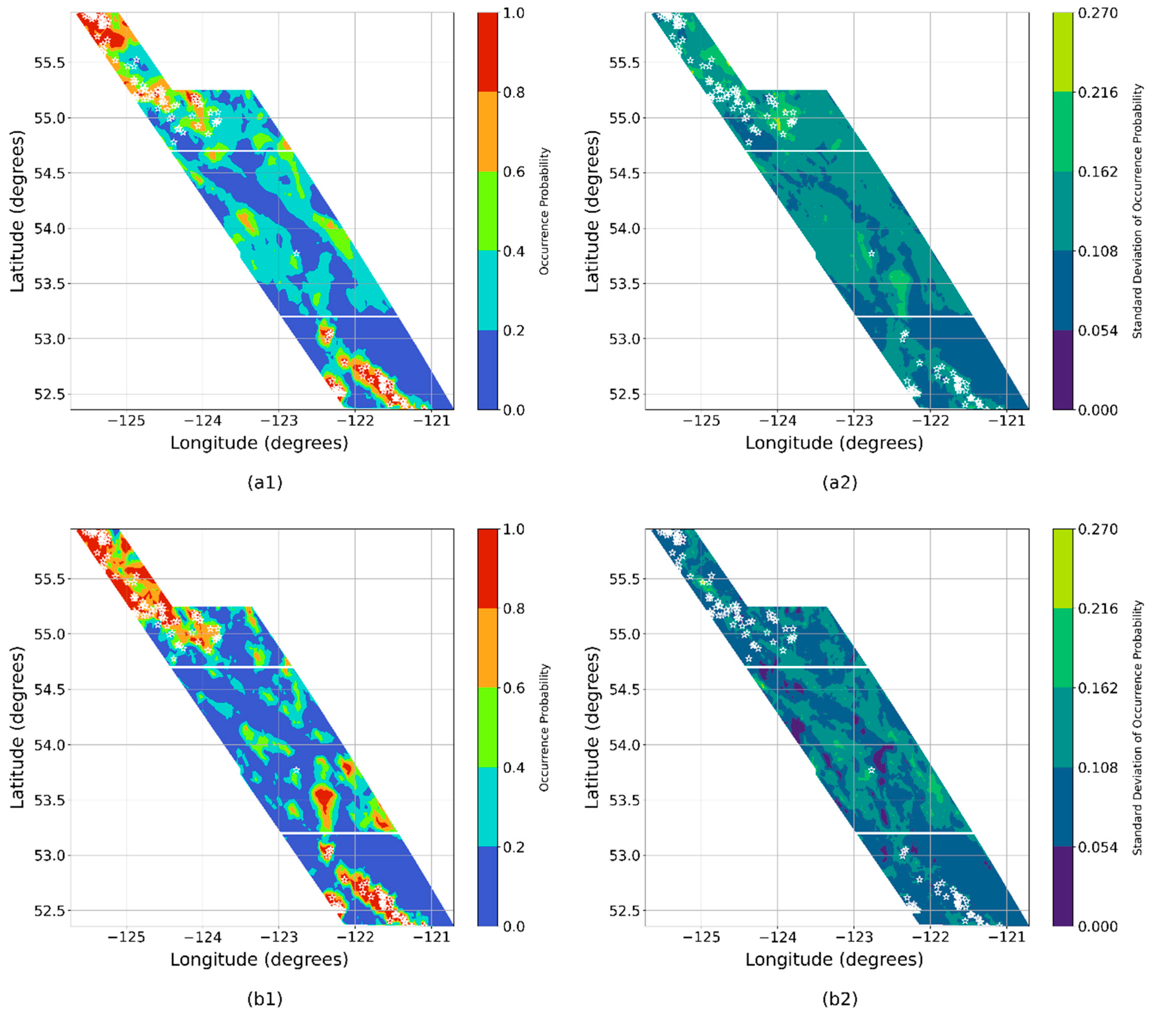
Interesting similarities and contrasts between the two optimized maps are observed (refer back to Figure 8 for subsequent references). The most prominent prediction is that of a highly prospective area at [−122.4 degrees East, 53.5 degrees North] after training on the optimal data features. This feature is totally absent in the unoptimized prospectivity map. However, the unoptimized prospectivity map contains an area of high variance in the same region, contrary to the optimized model, which produced significantly lower prediction variance in the region. Other features that exclusively appear in the optimized map include two small high prospectivity areas to the SouthEast and NorthEast of the feature at [−122.4 degrees East, 53.5 degrees North] (note that these features are coupled with relatively high standard deviations).

4. Discussion

The results of the input feature selection for our MPM problem have direct analogs to those of the binary classifier example outlined in Section 1. In the binary classifier problem, the input is an RGB image consisting of three color layers, with the green layer being altered. Therefore, in this context, the decision is to choose between the inclusion of the altered green layer together with the other two layers, or its full exclusion from the input feature set. The example showcases two types of scenarios: (1) random noise and (2) lack of meaningful correlation to labels and other input features. The former can represent MPM cases where some input features have logical correlation with labels and other features, yet contain noise. Uncertainty in determining geological age and ambiguity in the delineation of fault lines are examples of such a case. The optimal input feature set for our MPM excludes three out of four available geological features and their respective combinations. On the other hand, the inclusion of uncorrelated features into the input feature set (case 2) can be destructive to the training process. The lack of correlation can be purely logical and based on the particular mineral system of interest.
The optimal input feature set for our MPM problem includes VTEM and geochemical data, which have much higher spatial resolution and direct correlation to labels compared to features such as gravity and broad geological classifications, reflecting the scattered distribution of copper porphyry deposits and the nature of their underlying mineral system.
Optimal selection of input features for MPM has important implications for mineral exploration, especially for future survey planning. Although the optimal selection of input features is particular to the surveyed area, it can be a guide for future geophysical and geochemical surveys in adjacent regions or locations with similar structural geology and narrow down the list of necessary surveys for mineral prospectivity. In smaller-scale mineral exploration, data acquisition can be framed as a sequential decision-making problem, with the state being the available survey data and MPM validation metrics, and the action being the acquisition of a particular type of data at specific locations. However, the use of reinforcement learning remains challenging due to uncertainty in the design of the reward and the risk of the agent over fitting to local subtleties.

5. Conclusions

Modern computational tools, such as machine learning, capture sophisticated patterns in geoscientific data, generating robust prospectivity maps. This study successfully demonstrated the constructive effect of optimal input feature selection for CNN applications in copper porphyry prospectivity modeling of central interior British Columbia. The data selection optimization via the MAB results in noticeable improvements in model performance (6.8% better model performance and a 1.9% reduction in global model variance compared to using all available data) yet only requires 2.2% of the computational resources needed to exhaustively search for the optimal data subset. Future work can benefit from the use of recently developed recurrent attention models (RAMs) using deep reinforcement learning, which focus the attention of a convolutional neural network towards certain portions of the input features during the training process.

Author Contributions

A.K.: conceptualization, methodology, formal analysis and data interpretation, writing, and visualization. K.N.: methodology, data processing, review and editing. A.S.: project oversight and guidance, review and editing. All authors have read and agreed to the published version of the manuscript.

Funding

This research received no external funding.

Data Availability Statement

All data used in this research is public and cited in this manuscript. The code is made available upon reasonable request.

Conflicts of Interest

The authors declare no conflicts of interest.

Appendix A. CNN and MAB Parameters

Table A1. List of hyperparameters of the CNN in this study. CNN depth represents the total number of layers in the CNN’s neural network. FC depth is the number of fully connected layers in the CNN’s neural network. Dense size is the number of nodes in each layer of the CNN neural network. Dropout rate represents the rate at which some nodes of the fully connected layers are randomly deactivated. Learning rate is the rate at which the gradient of the loss function affects the network weights of the CNN during training. Total epochs are the number of times the CNN trains over the training labels. Patch size refers to the dimensions (in degrees) with which the geographic region under analysis is broken into small patches of area. Batch size refers to the size of the ensemble of patches that are used to update the CNN weights using the loss function at a time. Fmap size refers to the feature size of 1D CNN layers upon flattening. Kernel size refers to the dimensions of the kernel window. Stride size refers to the step size at which the kernel window moves and slides over the 2D inputs.
CNN depth5
FC depth2
Dense size16
Dropout rate0.1
Learning rate0.0001
Total epochs100
Patch size0.114°
Batch size32
αLRELU0.1
Fmap size64
Kernel size3
Stride size1
Table A2. ε-decay schedules and their respective expressions. N is the total number of MAB steps and n is the current step count.
Decay Schedule ε n
Linear ε n = 1 9 n 10 N
Exponential ε n = 10 n N
Rational ε n = N 2 N 2 + 9 n 2
Elliptical ε n = 9 1 n N 2 + 1 10

References

  1. Knox-Robinson, C.M.; Wyborn, L.A.I. Towards a holistic exploration strategy: Using Geographic Information Systems as a tool to enhance exploration. Aust. J. Earth Sci. 1997, 44, 453–463. [Google Scholar] [CrossRef]
  2. Reddy, R.K.T.; Bonham-Carter, G.F. A Decision-Tree Approach to Mineral Potential Mapping in Snow Lake Area, Manitoba. Can. J. Remote Sens. 1991, 17, 191–200. [Google Scholar] [CrossRef]
  3. Lawley, C.J.M.; Tschirhart, V.; Smith, J.W.; Pehrsson, S.J.; Schetselaar, E.M.; Schaeffer, A.J.; Houlé, M.G.; Eglington, B.M. Prospectivity modelling of Canadian magmatic Ni (±Cu±Co±PGE) sulphide mineral systems. Ore Geol. Rev. 2021, 132, 103985. [Google Scholar] [CrossRef]
  4. Cracknell, M.J.; Reading, A.M. Geological mapping using remote sensing data: A comparison of five machine learning algorithms, their response to variations in the spatial distribution of training data and the use of explicit spatial information. Comput. Geosci. 2014, 63, 22–33. [Google Scholar] [CrossRef]
  5. McMillan, M.; Haber, E.; Peters, B.; Fohring, J. Mineral prospectivity mapping using a VNet convolutional neural network. Lead. Edge 2021, 40, 99–105. [Google Scholar] [CrossRef]
  6. Yang, N.; Zhang, Z.; Yang, J.; Hong, Z. Applications of data augmentation in mineral prospectivity prediction based on Convolutional Neural Networks. Comput. Geosci. 2022, 161, 105075. [Google Scholar] [CrossRef]
  7. Li, Q.; Chen, G.; Luo, L. Mineral prospectivity mapping using attention-based convolutional neural network. Ore Geol. Rev. 2023, 156, 105381. [Google Scholar] [CrossRef]
  8. Krizhevsky, A.; Sutskever, I.; Hinton, G.E. ImageNet classification with deep convolutional Neural Networks. Commun. ACM 2017, 60, 84–90. [Google Scholar] [CrossRef]
  9. Cukierski, W. Dogs vs. Cats. Kaggle. 2013. Available online: https://kaggle.com/competitions/dogs-vs-cats (accessed on 15 March 2024).
  10. Sahu, R.K.; Müller, J.; Park, J.; Varadharajan, C.; Arora, B.; Faybishenko, B.; Agarwal, D. Impact of input feature selection on groundwater level prediction from a multi-layer perceptron neural network. Front. Water 2020, 2, 573034. [Google Scholar] [CrossRef]
  11. Hall, M.A. Correlation-Based Feature Selection for Machine Learning. Ph.D. Thesis, The University of Waikato, Hamilton, New Zealand, 1999. [Google Scholar]
  12. Egwu, N.; Mrziglod, T.; Schuppert, A. Neural network input feature selection using structured L2L_2L2-Norm Penalization. Appl. Intell. 2022, 53, 5732–5749. [Google Scholar] [CrossRef]
  13. Zhang, P. A novel feature selection method based on global sensitivity analysis with application in machine learning-based prediction model. Appl. Soft Comput. 2019, 85, 105859. [Google Scholar] [CrossRef]
  14. Rodríguez-Galiano, V.F.; Sánchez-Castillo, M.; Chica-Olmo, M.; Chica-Rivas, M. Machine learning predictive models for mineral prospectivity: An evaluation of neural networks, random forest, regression trees and support vector machines. Ore Geol. Rev. 2015, 71, 804–818. [Google Scholar] [CrossRef]
  15. Behnia, P.; Harris, J.; Sherlock, R.; Naghizadeh, M.; Vayavur, R. Mineral prospectivity mapping for orogenic gold mineralization in the Rainy River Area, Wabigoon Subprovince. Minerals 2023, 13, 1267. [Google Scholar] [CrossRef]
  16. Lou, Y.; Liu, Y. Mineral prospectivity mapping of tungsten polymetallic deposits using machine learning algorithms and comparison of their performance in the Gannan Region, China. Earth Space Sci. 2023, 10, e2022EA002596. [Google Scholar] [CrossRef]
  17. Lachaud, A.; Adam, M.; Mišković, I. Comparative study of random forest and support vector machine algorithms in mineral prospectivity mapping with limited training data. Minerals 2023, 13, 1073. [Google Scholar] [CrossRef]
  18. Kong, W.; Chen, J.; Zhu, P. Machine learning-based uranium prospectivity mapping and model explainability research. Minerals 2024, 14, 128. [Google Scholar] [CrossRef]
  19. Yang, S.; Yang, W.; Cui, T.; Zhang, M. Prediction and practical application of bauxite mineralization in Wuzhengdao area, Guizhou, China. PLoS ONE 2024, 19, e0305917. [Google Scholar] [CrossRef]
  20. Zhang, H.; Xie, M.; Dan, S.; Li, M.; Li, Y.; Yang, D.; Wang, Y. Optimization of feature selection in mineral prospectivity using ensemble learning. Minerals 2024, 14, 970. [Google Scholar] [CrossRef]
  21. Geoscience BC. Quest Project. 2020. Available online: https://www.geosciencebc.com/major-projects/quest/ (accessed on 1 July 2023).
  22. Mitchinson, D.E.; Fournier, D.; Hart, C.J.R.; Astic, T.; Cowan, D.C.; Lee, R.G. Identification of New Porphyry Potential Under Cover in British Columbia; Geoscience BC Report 2022-07, MDRU Publication 457; Geoscience BC: Vancouver, BC, Canada, 2022. [Google Scholar]
  23. Montsion, R.M.; Saumur, B.M.; Acosta-Gongora, P.; Gadd, M.G.; Tschirhart, P.; Tschirhart, V. Knowledge-driven mineral prospectivity modeling in areas with glacial overburden: Porphyry Cu exploration in Quesnellia, British Columbia, Canada. Appl. Earth Sci. 2019, 128, 181–196. [Google Scholar] [CrossRef]
  24. Shalev-Shwartz, S.; Ben-David, S. Stochastic Gradient Descent. In Understanding Machine Learning: From Theory to Algorithms; Cambridge University Press: Cambridge, UK, 2014; pp. 150–166. [Google Scholar] [CrossRef]
  25. Sutton, R.S.; Barto, A. Multi-armed Bandits. In Reinforcement Learning: An Introduction; The MIT Press: Cambridge, MA, USA, 2020; pp. 25–47. [Google Scholar]
  26. Dirkx, R.; Dimitrakopoulos, R. Optimizing Infill Drilling Decisions Using Multi-Armed Bandits: Application in a Long-Term, Multi-Element Stockpile. Math. Geosci. 2018, 50, 35–52. [Google Scholar] [CrossRef]
  27. Silva, N.; Werneck, H.; Silva, T.; Pereira, A.C.; Rocha, L. Multi-armed bandits in recommendation systems: A survey of the state-of-the-art and future directions. Expert Syst. Appl. 2022, 197, 116669. [Google Scholar] [CrossRef]
  28. Moeini, M. Orthogonal bandit learning for portfolio selection under cardinality constraint. In Computational Science and Its Applications—ICCSA 2019; Lecture Notes in Computer Science; Springer: Cham, Switzerland, 2019; pp. 232–248. [Google Scholar]
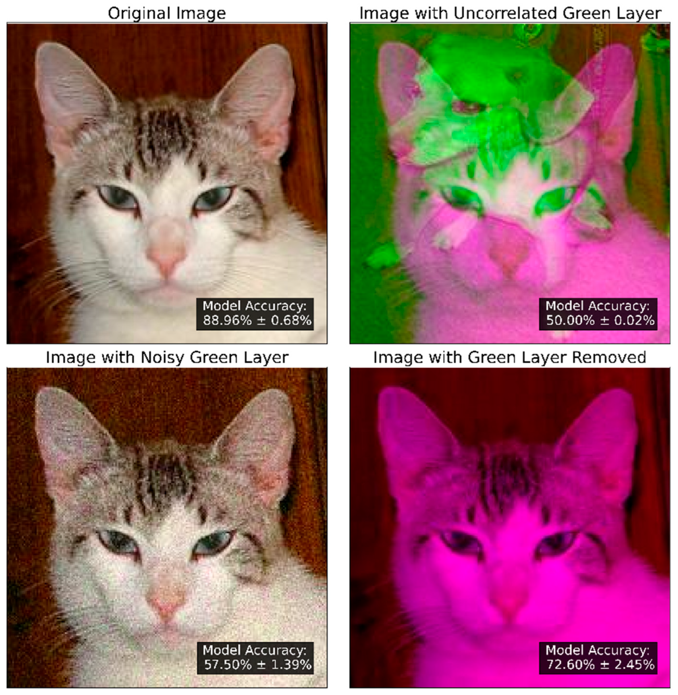
Figure 1. Validation performance of AlexNet cat/dog classifier trained on original and altered set of cat images. The green component of the cat images is either altered by the Gaussian noise (i.e., drawn from a Gaussian distribution around the original pixel value with a standard deviation equal to the noise intensity); or a full replacement with that of a random dog image. Alternatively, the green layer of the cat images can be fully removed prior to model training, leading to improved model accuracy.
Minerals 15 01237 g001
Figure 2. (Left) Normalized magnetic field strength data of central interior of British Columbia. (Right) Example of a data crop used as part of model training and validation (note that the axes are relative latitudes and longitudes.
Minerals 15 01237 g002
Figure 3. CNN architecture of the model used for copper porphyry prospectivity modeling in central interior British Columbia. Input features are pre-processed, uniformly cropped, and labeled according to the positions of known mineral occurrences in the region. Crops are 38 × 38 pixels, with a physical dimension of 19.1 km. This CNN consists of three components: input feature (red), five convolutional passes (green), and a fully connected artificial neural network (purple). After five convolutional passes and pooling has been performed, the obtained channels are flattened from a 2D format into a single 1D array. This array is used as the input of a fully connected artificial neural network, which returns an output layer. Note that the model uses a square loss function, and outputs regression scores as its predictions.
Minerals 15 01237 g003
Figure 4. Geometrical illustration of reward R. The reward aims to quantify how close the (TPR, FPR) at pthr = 0.5 is to the upper left corner (i.e., (TPR, FPR) = (0, 1)). This notion is roughly equivalent to how far this point is from the bottom right corner of the graph (i.e., (TPR, FPR) = (1, 0)). Thus, distance d is first calculated, normalized by dmax = 2 , and subtracted by 1 to obtain the equivalent normalized distance from (TPR, FPR) = (0, 1).
Minerals 15 01237 g004
Figure 5. MAB algorithm applied to input feature selection for a CNN model training and validation process. This diagram represents one step of the MAB algorithm.
Minerals 15 01237 g005
Figure 6. (Upper) Mean reward matrix of all data subsets after an exhaustive search (i.e., 180 trainings per training feature subset). The null combination is marked by the phi symbol. The most optimal data combination is boxed in green, and the configuration that includes all data types is boxed in blue. (Lower) Standard deviation of model reward over the 180 training iterations per input feature subset.
Minerals 15 01237 g006
Figure 7. (Left) ε-decay schedules. (Right) Sample of the reward evolution represented by a 60-step moving average for different ε-decay schedules over a 525-step window.
Minerals 15 01237 g007
Figure 8. Copper porphyry prospectivity of central interior British Columbia. (a1,a2) Average and standard deviation prospectivity maps of CNN models trained on all feature types, respectively. (b1,b2) Average and standard deviation prospectivity maps of CNN models trained on the optimal subset of feature types selected by the MAB. The CNN was trained 180 times independently on each training feature. Models are trained on the labels south of the 53.2 degrees latitude and validated on the labels north of 54.7 degrees from their respective features (marked by horizontal white lines). White star marks indicate known mineral occurrence locations.
Minerals 15 01237 g008
Table 1. Indicators for the QUEST data subsets.
0No Geological DataA0No Geophysical & No Geochemical Data
1Geological ClassA1Geochemistry
2Geological SubclassB0Gravity
3Geological AgeB1Gravity & Geochemistry
4Distance to Nearest FaultC0Magnetics
5Geological Class & SubclassC1Magnetics & Geochemistry
6Geological Class & AgeD0VTEM
7Geological Class & Distance to Nearest FaultD1VTEM & Geochemistry
8Geological Subclass & AgeE0Gravity & Magnetics
9Geological Subclass & Distance to Nearest FaultE1Gravity, Magnetics & Geochemistry
10Geological Age & Distance to Nearest FaultF0Gravity & VTEM
11Geological Class, Subclass & AgeF1Gravity, VTEM & Geochemistry
12Geological Class, Subclass & Distance to Nearest FaultG0Magnetics & VTEM
13Geological Class, Age & Distance to Nearest FaultG1Magnetics, VTEM & Geochemistry
14Geological Subclass, Age & Distance to Nearest FaultH0Gravity, Magnetics & VTEM
15Geological Class, Subclass, Age & Distance to Nearest FaultH1Gravity, Magnetics, VTEM & Geochemistry
Disclaimer/Publisher’s Note: The statements, opinions and data contained in all publications are solely those of the individual author(s) and contributor(s) and not of MDPI and/or the editor(s). MDPI and/or the editor(s) disclaim responsibility for any injury to people or property resulting from any ideas, methods, instructions or products referred to in the content.