Evaluation of Heterogeneous Ensemble Learning Algorithms for Lithological Mapping Using EnMAP Hyperspectral Data: Implications for Mineral Exploration in Mountainous Region

Abstract

Hyperspectral remote sensing plays a crucial role in guiding and supporting various mineral prospecting activities. Combined with artificial intelligence, hyperspectral remote sensing technology becomes a powerful and versatile tool for a wide range of mineral exploration activities. This study investigates the effectiveness of ensemble learning (EL) algorithms for lithological classification and mineral exploration using EnMAP hyperspectral imagery (HSI) in a semi-arid region. The Moroccan Anti-Atlas mountainous region is known for its complex geology, high mineral potential and rugged terrain, making it a challenging for mineral exploration. This research applies core and heterogeneous ensemble learning methods, i.e., boosting, stacking, voting, bagging, blending, and weighting to improve the accuracy and robustness of lithological classification and mapping in the Moroccan Anti-Atlas mountainous region. Several state-of-the-art models, including support vector machines (SVMs), random forests (RFs), k-nearest neighbors (k-NNs), multi-layer perceptrons (MLPs), extra trees (ETs) and extreme gradient boosting (XGBoost), were evaluated and used as individual and ensemble classifiers. The results show that the EL methods clearly outperform (single) base classifiers. The potential of EL methods to improve the accuracy of HSI-based classification is emphasized by an optimal blending model that achieves the highest overall accuracy (96.69%). The heterogeneous EL models exhibit better generalization ability than the baseline (single) ML models in lithological classification. The current study contributes to a more reliable assessment of resources in mountainous and semi-arid regions by providing accurate delineation of lithological units for mineral exploration objectives.

1. Introduction

Lithological mapping is a crucial step toward effective mineral exploration in mountainous and remote regions. The use of hyperspectral remote sensing imagery for lithological mapping is a practical and powerful tool for the accurate identification of potential mineral zones. Several airborne and spaceborne hyperspectral sensors, including the digital airborne imaging spectrometer, Hyperion, the hyperspectral digital imagery collection experiment (HYDICE), the advanced visible infrared imaging spectrometer (AVIRIS), HyMap (hyperspectral mapper), and PRecursore IperSpettrale della Missione Applicativa (PRISMA), as well as the recently launched Environmental Mapping and Analysis Program (ENMAP), have been extensively used for lithological mapping and mineral exploration [1,2,3,4,5,6,7].

Hyperspectral remote sensing technology becomes a powerful and versatile tool for a wide range of mineral exploration activities. Ensemble learning (EL) techniques in remote sensing for mineral exploration have gained increasing recognition and much attention, as they can improve the accuracy and robustness of lithological and mineral mapping [8,9]. Conventional single machine learning (ML) models (e.g., SVM and KNN) often struggle with complex, nonlinear relationships and imbalanced data structures, which limits their performance on lithological classification tasks [10]. Ensemble learning represents a paradigm shift in predictive modeling, offering enhanced accuracy [11], a particularly valuable approach when dealing with heterogeneous datasets and the inherent complexity of the outcrop. Traditional ML algorithms, e.g., support vector machines (SVMs), random forest (RF), k-nearest neighbors (k-NNs), decision trees (DT), extreme gradient boosting (XGB), and artificial neural networks (ANNs) have demonstrated considerable success in lithological classification using hyperspectral data [12,13,14,15]. EL methods capitalize on their individual strengths, harmonizing them into a collective framework that mitigates model-specific biases and achieves superior classification performance.

The models mentioned above utilize the rich spectral information of different hyperspectral images to capture subtle variations in mineral and rock composition. For example, SVMs are particularly well suited to construct complicated decision boundaries (i.e., an optimal separating hyperplane) in a high-dimensional feature space to ensure precise separability of classes. RF utilizes ensemble learning to improve resilience to noise and variability in the data. Despite its basic nature, k-NN (an instance-based classifier) remains a powerful lazy learner that excels in classification scenarios where the spectral clusters are clearly structured. However, these heterogeneous traditional machine learning models face significant challenges when dealing with the inherent high dimensionality of hyperspectral data (i.e., the curse of dimensionality) [16,17]. In addition, many traditional ML models have difficulty capturing the nonlinear relationships and multimodal structure of geological data, making it difficult to accurately classify complex lithological features. EL methods (i.e., multiple classifiers) can improve prediction accuracy and robustness by leveraging the strengths of individual models through the combination of their predictions [18]. EL models are characterized by improved classification performance, effective handling of unbalanced data, and reduced overfitting. The seamless integration of sophisticated ensemble models combined with robust feature techniques remains essential for improving the accuracy and reliability of lithological mapping in remote sensing.

The fundamental types of ensemble models are as following: voting, bagging, boosting, and stacking, each with unique approaches to integrate model predictions. Voting (or majority voting) gathers predictions from diverse ML models by averaging their probabilities (soft voting) or taking the most frequent class prediction (hard voting), aiming to reduce baseline algorithms errors and then improve overall robustness [19]. Bagging (Bootstrap Aggregating), used in random forest, reduces variance and prevents overfitting by training models on randomly sampled subsets of the data and combining their decision boundaries, typically through averaging or majority voting [20]. Additionally, boosting methods, such as Gradient Boosting Machines (GBMs), AdaBoost, and XGBoost/XGB (extreme gradient boosting), improve model performance iteratively, with each new model focusing on mitigating the errors of the previous ones [21]. Stacking combines multiple models by fitting a meta-learner that calculates the final prediction based on the outputs of the base models, leveraging their distinct strengths in order to produce improved accuracy [22]. Further methodological details and performance evaluations of these models are comprehensively presented in Section 3.

Numerous studies have substantiated the efficacy of ensemble learning paradigms such as boosting, bagging, and stacking in classification/regression tasks within remote sensing data analysis, owing to their capacity to enhance predictive performance and generalization [23]. However, their systematic deployment in hyperspectral lithological discrimination remains insufficiently explored. More specifically, conventional homogeneous ensemble models, including RF and XGB, have been widely explored in lithological and mineralogical mapping, capitalizing on their robustness and their ability to model spectral patterns, e.g., [24,25,26,27]. In contrast, heterogeneous ensemble frameworks, which combine diverse learning algorithms instead of relying on multiple iterations of a single model type, remain underutilized in hyperspectral geological studies, with relatively few published works in this area. For instance, Lin, Liu [28] employed the Sparrow Search Algorithm (SSA) alongside two ML algorithms, RF and Gradient Boosting Decision Tree (GBDT) to enhance mineral mapping using ZY1-02D HSI for the Qinghai Gouli region (China). Using non-imagery data, Farhadi, Tatullo [29] demonstrated a valuable impact of heterogeneous EL for lithological mapping using geochemical and geological data, revealing that stacking ensemble methods yielded the highest Cohen’s kappa and Matthews correlation coefficient (MCC) scores, indicating their effectiveness in handling complex geological data. For mineral prospectivity mapping, a recent study by Remidi, Boutaleb [30] proposed an amalgamation of machine learning and deep learning methodologies, illustrating the impact of a stacking ensemble technique in forecasting Pb-Zn mineral deposits within the Northeastern region of Algeria. The model attained a ROC-AUC exceeding 98%, underscoring the dominant influence of tectonic dynamics and metallogenic mechanisms in the metallogenies model. The research gap on the application of heterogeneous EL warrants further investigation to elucidate their potential for improving classification accuracy and interpretability in hyperspectral-driven lithological assessments.

The current work provides critical insights for advancing the field of lithological and mineral mapping, particularly given the limited research on EnMAP hyperspectral imagery for lithological mapping using heterogeneous ensemble learning models. We aim to address the shortcomings/drawbacks of the traditional machine learning approaches by exploring the potential of heterogeneous ensemble learning techniques. By systematically evaluating the performance of various ensemble models in geological classification tasks, the current research seeks out to establish a more robust framework for integrating hyperspectral data with traditional ML along with EL techniques. This approach is especially significant in regions where geological data is sparse, as accurate mapping is a prerequisite for effective preliminary resource exploration. The primary objectives of this experimental research are as follows: (1) to evaluate the effectiveness of various heterogeneous ensemble learning techniques (stacking, voting, blending, etc.) in improving the accuracy and robustness of lithological classification using EnMAP hyperspectral data; (2) to perform a comprehensive benchmark of the various EL methods; (3) to develop a framework for integrating ensemble learning and HSI remote sensing data to enhance geological mapping accuracy in complex (highly altered) and mountainous regions. Through these objectives, we aim to bridge the gap between traditional ML models and advanced ensemble methods, paving the way for more accurate geological mapping in analogous regions worldwide.

2. Geology of the Study Area

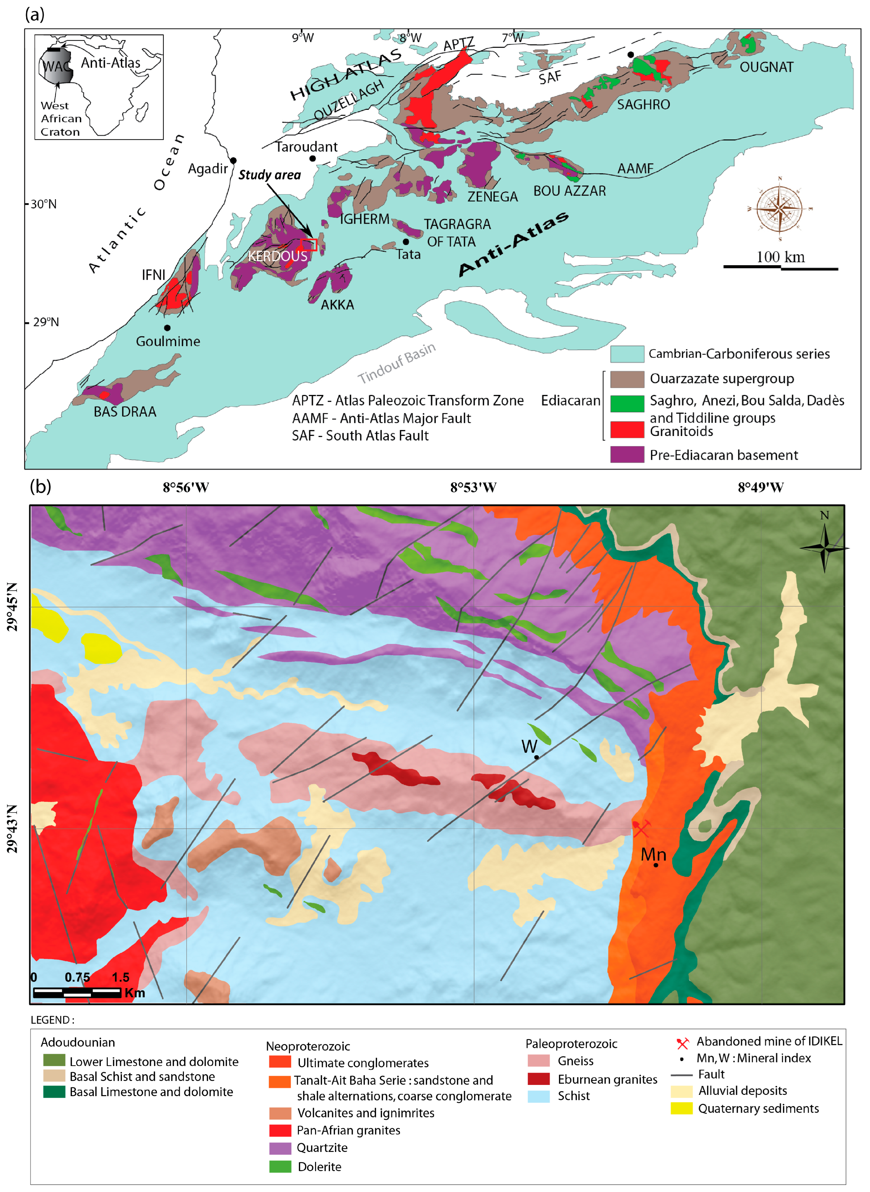
Study area is located in the northwestern region of the West African Craton (WAC) (Figure 1a). More specifically, the area is located in the Anti-Atlasic belt, which is composed of a Proterozoic basement outcrops and inliers, e.g., Kerdous, Bas-Draa, Saghro, Bou-Azzer, Ifni, and Ighrem. These inliers are hidden under a Ediacaran-Paleozoic cover in the western Anti-Atlas [31,32]. The current study was conducted along the eastern border of the Kerdous inlier and intersects the site of the abandoned Idikel mine (Figure 1b). Within the basement units, the Paleoproterozoic is dominated by polymetamorphic rock complexes [33]. They are formed by the orthogneisses of Jbel Ouiharen (Xoε), as well as schists, mica-schists, and blastomylonites (XIξ, luXII2). These units are overlain by several granitoids, including the Tasserhirt Plateau granite (XIm). The Neoproterozoic comprises quartzites (northern study area represented by Jbel Lkest quartzites (XII2q)), rhyolitic volcanites and ignimbrites (XIIIm), from the Adrar Mkorn Mountain area Tafraout granites (XII3γ), and volcano-detrital deposits (XIIIS1), materialized essentially with sandstone-shale (XIIIS1e), as well as conglomerates (XIIIS1cg). This ensemble is overlain by XIIIS2 as the ultimate conglomerates of the base of Adoudou series according to Hassenforder [33]. Doleritic veins (XII2) frequently occur within quartzites. The Paleozoic cover unconformably overlies the Proterozoic lithofacies [34]. In the study area, this cover begins with the basal series “serie de base” as a lower member, which consists of schists and sandstones (Ad11a), limestones, and dolomites (Ad11b). Above this, the upper member of carbonates is represented by the lower series “serie inferieure”, occurring in the eastern study area as dolomites and limestones (Ad12).

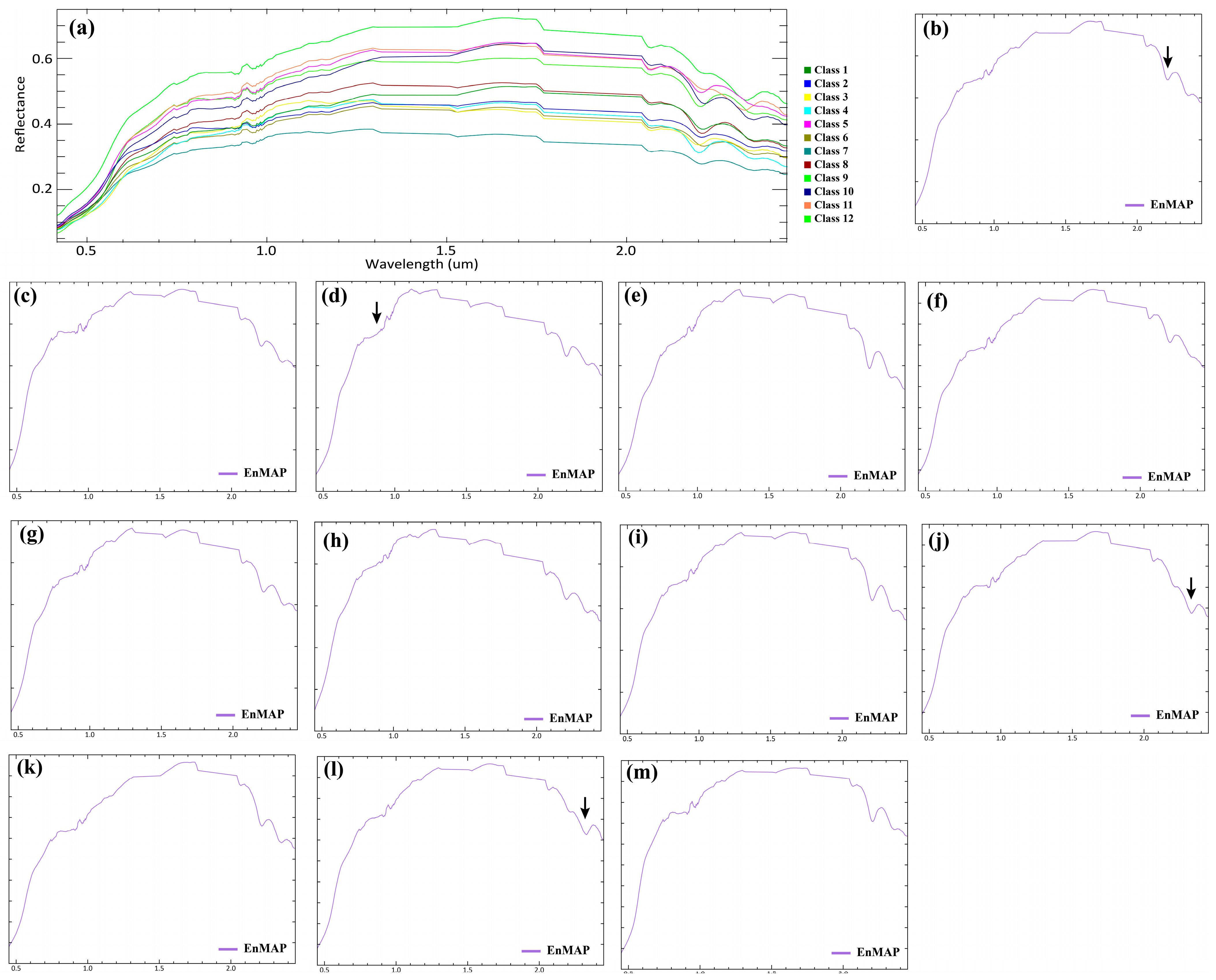
From a metallogenic standpoint, the Eastern Kerdous inlier is an area known for its copper and manganese deposits [35,36]. The study area has been thoroughly examined in previous remote sensing investigations, which have provided insights into Neoproterozoic to Cambrian copper mineralization in the surrounding area. These studies also identified significant alteration processes, including argillic, phyllic, and silicification [27,35]. Alteration spectral features have been highlighted with airborne spectroscopy data, as well as captured in several rock classes mean spectra (Figure 2a). Figure 2b,d,j,l reveal the spectral features of Al-OH, Fe²⁺, and Mg-Fe-OH (Figure 2j,l), respectively.

Figure 1. Geological setting of the Kerdous inlier in the southwestern Anti-Atlas, showing its location on the map of the Moroccan Anti-Atlasic Belt (a) [37], and the geological map of the study area (b), extracted from the Tafraout map (1:100,000) (modified from [27]).

Figure 1. Geological setting of the Kerdous inlier in the southwestern Anti-Atlas, showing its location on the map of the Moroccan Anti-Atlasic Belt (a) [37], and the geological map of the study area (b), extracted from the Tafraout map (1:100,000) (modified from [27]).

Figure 2. (a) Mean spectral signatures of 12 lithological units (refer to Table S1 for more details regarding classes corresponding formations) in the eastern Ameln Valley Shear Zone (AVSZ). The black arrows in the subplots (b–m) highlight the spectral features related to alteration minerals occurrences in the eastern Kerdous region for the 12 mapped units (class1–class12, respectively) as previously revealed in [38,39].

Figure 2. (a) Mean spectral signatures of 12 lithological units (refer to Table S1 for more details regarding classes corresponding formations) in the eastern Ameln Valley Shear Zone (AVSZ). The black arrows in the subplots (b–m) highlight the spectral features related to alteration minerals occurrences in the eastern Kerdous region for the 12 mapped units (class1–class12, respectively) as previously revealed in [38,39].

3. Materials and Methods

3.1. EnMAP Hyperspectral Dataset and Ground-Truth Information

The EnMAP satellite mission, created to support thorough global environmental observation and analysis, was launched on 1 April 2022 [40]. This system is an imaging push broom setup equipped with two spectrometers that capture spectral data within the 420 to 2450 nm wavelength range [41]. The hyperspectral EnMAP imager has a 30 m spatial resolution and a swath width of 30 km, offering spectral resolutions of 6.5 nm and 10 nm, respectively, in the VNIR and SWIR. The sensor also boasts an impressive signal-to-noise ratio (SNR) of 400:1 at 495 nm and 170:1 at 2200 nm [42].

In this study, we used a cloud free EnMAP image (Level 2A EnMAP product atmospherically and geometrically corrected), georeferenced using the Universal Transverse Mercator, 29N, with the WGS84 datum. The scene, originally centered at coordinates (Origin = −9.201435, 29.924735), was acquired on 9 August 2023 at 12:07:02 UTC. This scene was subsequently resized and clipped to focus on the eastern Kerdous area, specifically covering the Idikel mine region. This targeted spatial refinement ensured that the analysis concentrated on the lithologically diverse and mineralogically significant zones relevant to the study objectives. Before applying classification algorithms, bands within the range of 1780.22–1967.66 nm were removed (anomalous bands), as well as the anomalous band at 2005.08 nm, along with the water absorption bands from 1330.85 to 1495.89 nm and 1780.22 to 2032.7 nm. After these exclusions, 204 bands were retained for further processing. Furthermore, this study adopts lithological mapping with 12 lithological classes to categorize the various rock types identified within the study area. Each class is assigned a distinct code for identification, as defined in the Tafraout geological map. The 12 classes are Class 1 (Orthogneisses), Class 2 (schist, mica-schist, gneiss, blastomylonites), Class 3 (dolerite), Class 4 (quartzites), Class 5 (granites—Tafraout), Class 6 (vulcanites and ignimbrites), Class 7 (greso-pelitic series with tuffs and local red limestone, conglomerates, and coarse conglomerates), Class 8 (conglomerates—Ultimate), Class 9 (limestone and dolomites—basal series), Class 10 (schist and sandstone—basal series), Class 11 (limestone and dolomites—lower series), and Class 12 (Quaternary deposits). The ground truth records consist of 5631 pixels, for a total classified area of 156,045 pixels [6].

3.2. Baseline Classification Algorithms

All experiments were conducted using a Python (3.11.13) environment, which is flexible for ML-based processing. The implementation leveraged a wide range of scientific and machine learning libraries, including NumPy, Pandas, Scikit-learn, Matplotlib, Seaborn, Plotly graphing, as well as the Rasterio package. Ensemble and conventional classifiers were built and implemented by means of Scikit-learn (v.1.6.1).

3.2.1. Support Vector Machines (SVM)

A Support Vector Machine (SVM) is a kernel-based learning algorithm that aims to find the optimal hyperplane that separates data points of different classes [43]. SVMs were primarily designed for separating two linearly separable classes. In cases where the classes are not linearly separable, SVM uses kernel functions (kernel trick) to map the data into higher-dimensional feature spaces, enabling non-linear classification to separate the classes. The decision boundary is determined by support vectors data points closest to the hyperplane by maximizing the margin space between two classes. SVM is an effective method for high-dimensional data classification and is robust against overfitting issues, especially when using regularization techniques.

3.2.2. k-Nearest Neighbors (KNNs)

k-Nearest Neighbors (KNNs) is a non-parametric instance-based learning algorithm and makes no assumption regarding the underlying data distribution. The method predicts the class of a data point based on the majority class among its k-nearest neighbors [44]. The distance metric (e.g., Euclidean, Manhattan) determines similarities between data points. KNN is simple and effective for small datasets but can be computationally expensive for large datasets, requiring parameter optimization such as KD-trees or Ball trees for efficiency and improved accuracy.

3.2.3. Multi-Layer Perceptron (MLP)

Multi-Layer Perceptron (MLP) is a class of artificial neural networks consisting of multiple layers of interconnected neurons [45]. MLP uses backpropagation to update weights through gradient descent, allowing it to learn complex non-linear relationships. Activation functions such as ReLU and sigmoid enhance learning capabilities [46]. MLPs are widely used in deep learning (DL) but require careful tuning of hyperparameters to avoid overfitting (tuned hyperparameters optimization has been inserted Appendix A).

3.2.4. Decision Trees (DTs)

A Decision Tree (DT) is a tree-based learning algorithm that recursively splits the data based on feature thresholds to maximize class separation [47]. The splitting criterion (e.g., Gini impurity, entropy) determines the quality of the splits. DTs are interpretable and computationally efficient but prone to overfitting unless pruned or regularized [48], while random forests-like models are ensemble methods that combine multiple DTs to improve accuracy and generalization. In this context, we specifically assessed both DT and RF models in our study area (see Section 3.3), where their performances were compared in terms of lithological classification accuracy.

3.3. Homogeneous EL

3.3.1. Bagging

Also known as Bootstrap Aggregating, bagging is a machine learning technique designed to enhance the accuracy and stability of classification and regression models. It achieves this by reducing variance and minimizing the risk of overfitting. The process involves generating multiple subsets of the training data through random sampling with replacement. Each of these subsets, known as bootstrap samples, is used to train a separate classifier of the same type. The final prediction is made by aggregating the outputs of all individual classifiers, typically through a majority vote, to determine the most likely outcome [49].

Random forest (RF) is an EL method based on decision trees, where multiple trees are trained on bootstrapped samples of the data, and the final prediction is obtained by averaging (for regression) or majority voting (for classification) [50]. RF reduces overfitting compared to single decision trees and improves generalization by introducing randomness in both data selection and feature selection. The algorithm is highly robust and performs well with high-dimensional data [24]. RF also provides strong performance in RS data analysis in terms of classification and regression. It is highlighted for its high classification accuracy, non-parametric nature, and ability to estimate variable importance. It is robust to noise and reductions in training data, and it requires fewer hyperparameters to be defined, simplifying the tuning process compared to the SVM classifier [51,52].

Bagging–Decision Trees (Bagging–DT) is an ensemble learning technique that trains multiple decision trees on different bootstrapped samples of the data and aggregates their predictions [53]. Bagging reduces variance and improves model stability, making it more robust to noise and overfitting compared to a single decision tree.

Extremely Randomized Trees (ETs), also known as extra trees, is a tree-based ensemble method that introduces additional randomness by selecting feature splits completely at random instead of optimizing a criterion [54]. This reduces variance further while maintaining computational efficiency, making ET an alternative to random forest.

3.3.2. Boosting

Boosting algorithms are iterative algorithms based on the progressive improvement of a model’s predictive quality by combining multiple weak models to create a more robust and efficient model. Their principle relies on training a series of weak models sequentially, giving more importance to the errors made by previous models. Each new model attempts to correct the errors of the previous one by assigning more weight to the misclassified observations [55].

Adaptive Boosting (AdaBoost) is a boosting technique that combines multiple weak classifiers, typically decision trees, by assigning higher weights to misclassified samples in each iteration [56]. The final classifier is a weighted sum of the weak classifiers, improving predictive accuracy. AdaBoost is sensitive to noisy data but works well for moderately complex datasets.

Extreme gradient boosting (XGBoost) is an optimized gradient boosting algorithm designed for speed and performance [57]. XGBoost minimizes loss through a gradient descent approach and includes regularization terms to prevent overfitting. It is widely used in machine learning competitions due to its efficiency and predictive power.

Histogram-based gradient boosting (HistGBT) represents an optimized form of traditional gradient boosting, designed to enhance computational efficiency by transforming continuous input variables into a finite set of discrete bins [58]. This discretization approach markedly lowers both memory demands and processing time, rendering HistGBT particularly advantageous for handling extensive datasets. The algorithm incorporates sophisticated capabilities, such as intrinsic support for missing data and the enforcement of monotonic relationships, thereby broadening its applicability and bolstering its performance across a wide array of recent predictive modeling challenges [59,60].

3.4. Heterogeneous EL Methods

3.4.1. Voting

Voting is a fundamental ensemble-learning method that combines predictions from multiple base classifiers to improve overall performance [61]. The flowchart of the voting ensemble is shown in Figure 3. This technique can be categorized into two types: hard voting and soft voting. In hard voting, each classifier casts a vote for a predicted class, and the class with the majority votes is selected as the final output. In soft voting, the predicted probabilities of each classifier are averaged, and the class with the highest probability is chosen. Voting is particularly effective when the base classifiers are diverse, as it leverages their complementary strengths to reduce individual biases and variance. In this study, the soft voting method was employed, where the final prediction is based on the highest value of the weighted average of the predicted probabilities. Notably, the implemented approach does not require any hyperparameter tuning.

3.4.2. Stacking

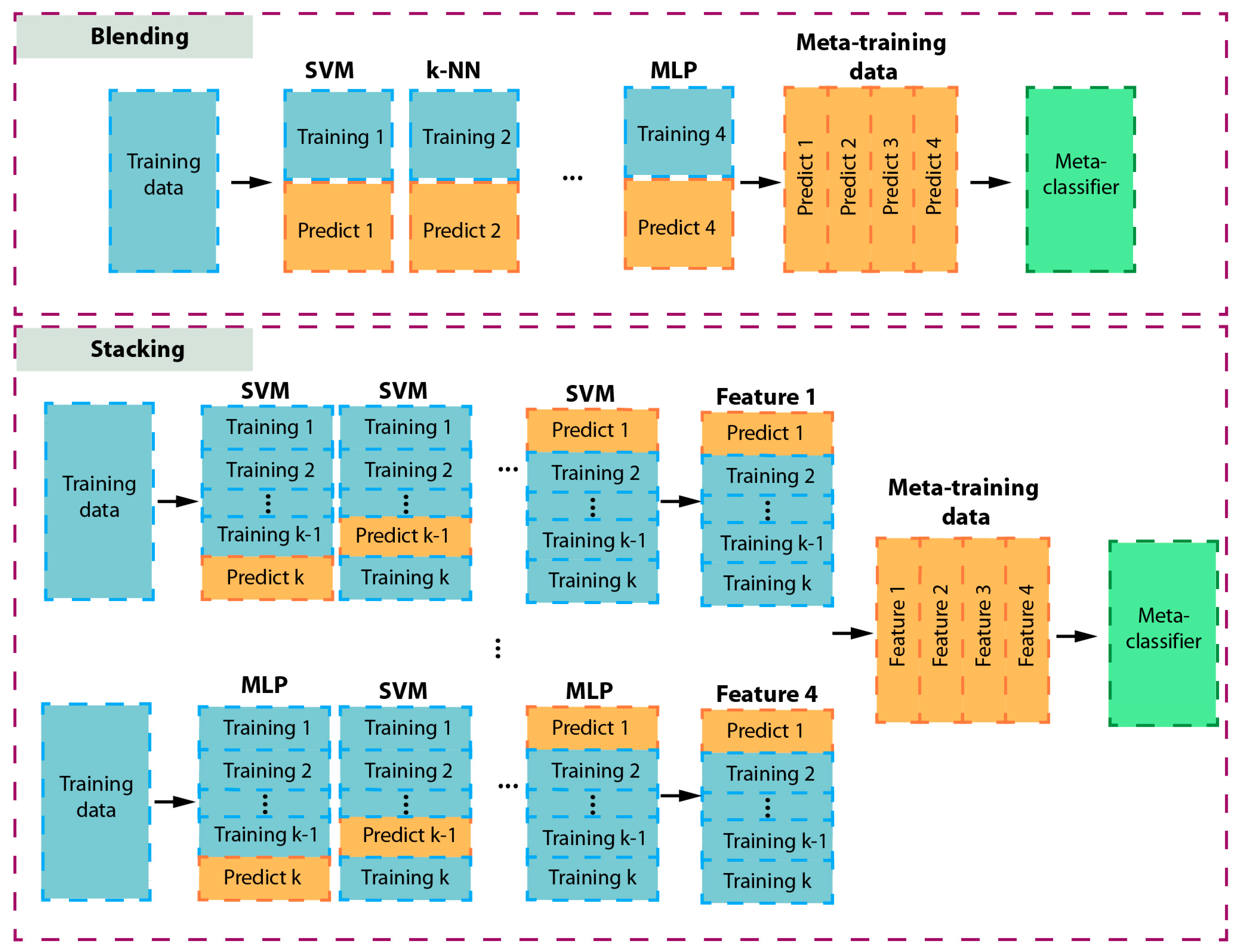
Stacking is a popular heterogeneous ensemble-learning technique that can use meta-models to combine different base classifiers for more accurate prediction results [62]. Figure 4 illustrates the flowchart of the stacking ensemble. The stacking method consists of the following steps: (1) train multiple base classifiers using K-fold cross-validation on the training set; (2) collect the output predictions (feature vectors) from these base classifiers to create a new training dataset; (3) train a meta-classifier on this new dataset. Stacking can collectively estimate errors from all base classifiers through the base-learning phase and refine predictions through the meta-learning phase, thereby reducing residual errors. In this study, logistic regression was utilized as the meta-classifier for generating the final susceptibility prediction. Notably, this implementation does not require hyperparameter tuning for the stacking method.

3.4.3. Weighting

Weighting is an ensemble-learning method in which different classifiers contribute to the final prediction with different importance levels [63]. The weighting ensemble’s flowchart is shown in Figure 5. Instead of treating each model equally, weighting assigns a confidence score to each classifier based on its performance on a validation set. The final prediction is computed as a weighted combination of the individual predictions. Common weighting strategies include accuracy-based weighting, entropy weighting, and Bayesian model averaging. This approach improves robustness by prioritizing stronger models while still leveraging insights from weaker classifiers. In this study, accuracy-based weighting was utilized as the weighting strategy.

3.4.4. Blending

Blending is a variant of stacking that uses a holdout validation set to train the meta-model instead of K-fold cross-validation [64]. Figure 4 illustrates the mechanism of the blending ensemble. Blending reduces information leakage compared to stacking and is computationally more efficient, though it requires sufficient validation data to generalize well. The process consists of the following steps: (1) split the training data into two subsets, typically 70% for training and the rest for validation; (2) train base classifiers on the training subset and generate predictions on the validation subset; (3) use these predictions as input features for the meta-model, which is then trained on the validation subset; (4) use the trained meta-model to make final predictions. Logistic regression was utilized as the meta-classifier for generating the final susceptibility prediction.

It is important to emphasize that hyperparameter tuning during the training phase is crucial for ensuring the convergence of models toward optimal parameters. This process, conducted within the main parameter ranges for each model, significantly enhances model performance, leading to optimal accuracy. Accordingly,

Table A1. Hyperparameter optimization via Python-implemented grid search cross-validation: optimal configurations for enhanced model accuracy.

Base Classifier	Hyperparameters	Optimized Parameter
SVM	C	10
	gamma	0.01
	kernel	rbf
KNN	n_neighbors	11
	weights	distance
	distance	2
	algorithm	auto
	Leaf_size	10
RF	n_estimators	200
	max_features	sqrt
	max_depth	None
	min_samples_split	2
	min_samples_leaf	1
DT	criterion	entropy
	max_depth	None
	min_samples_split	2
	min_samples_leaf	1
	max_features	None
Bagging–DT	Estimator	DT
	n_estimators	200
	max_samples	1.0
	max_features	0.5
MLP	hidden_layer_sizes	(150, 100, 50)
	activation	‘tanh’
	solver	‘adam’
	alpha	0.001
	learning_rate	‘constant’
	max_iter	100
AdaBoost	estimator	DT
	n_estimators	200
	learning_rate	1.0
	estimator__max_depth	3
XGBoost	n_estimators	200
	max_depth	6
	learning_rate	0.1
	subsample	0.8
	colsample_bytree	0.8
	gamma	0
Histogram-Based GBM	max_iter	200
	learning_rate	0.1
	max_depth	15
	min_samples_leaf	30
Extra Trees	n_estimators	200
	max_depth	None
	min_samples_split	2
	min_samples_leaf	1

presents the hyperparameter tuning details for the base classifiers. Hyperparameter tuning is a critical step in machine learning to ensure models converge toward their optimal configurations, maximizing predictive performance. This process involves the grid search application to identify the best combination of hyperparameters for each algorithm [65,66]. Proper tuning mitigates overfitting and enhances generalization, as demonstrated in studies where optimized hyperparameters improved model accuracy [67].

3.5. Accuracy Analysis

For accuracy assessment, we employed multiple evaluation methods to gauge the performance of our classification algorithms. The dataset was initially partitioned into training and testing subsets using a conventional 70-30 split, ensuring a balanced representation of samples. To comprehensively evaluate model effectiveness, we computed various metrics, including overall accuracy (OA), average accuracy (AA), recall, F1-score, kappa coefficient (k), user accuracy “Precision”, and producer accuracy “Recall” [68]. The corresponding equations for each of these evaluation metrics are outlined below. It is noteworthy that in remote sensing datasets classification accuracy, it is common to assess and quantify the commission error and the omission error easily via user and producer accuracies, respectively (Commission Error = 100 − User accuracy; Omission Error = 100 − Producer accuracy).

$$\mathrm{OA}={\displaystyle \frac{TP+TN}{TP+FP+TN+FN}}$$

(1)

$$\mathrm{AA}={\displaystyle \frac{1}{N}}\sum _{i=1}^N{\displaystyle \frac{T{P}_i}{T{P}_i+F{N}_i}}$$

(2)

$$\mathrm{Recall}={\displaystyle \frac{TP}{TP+FN}}$$

(3)

$$\mathrm{Precision}={\displaystyle \frac{TP}{TP+FP}}$$

(4)

$$\mathrm{F}1={\displaystyle \frac{2\cdot \mathit{Precision}\cdot \mathit{Recall}}{\mathit{Precision}+\mathit{Recall}}}$$

(5)

$$\mathsf{\kappa }={\displaystyle \frac{OA-P_e}{1-P_e}}$$

(6)

With, the expected agreement ($P_e$):

$$P_e={\displaystyle \frac{\left(TP+FP\right)\left(TP+FN\right)+\left(FN+TN\right)\left(FP+TN\right)}{{\left(TP+FP+TN+FN\right)}^2}}$$

(7)

where TP, TN, FP, and FN represent true positive, true negative, false positive, and false negative values, respectively.

In scenarios with imbalanced datasets, where all classes are equally important, we employed the macro-average method (Equation (8)).

$$MacroAvg(M)={\displaystyle \frac{1}{C}}\sum _{i=1}^c M_i$$

(8)

where Mi is the metric (e.g., precision, F1-score…) for class i, and C is the total number of classes.

This approach assigns equal weight to each class, ensuring a balanced evaluation across all categories. Accordingly, the F1 scores were computed using the macro-average method to provide a fair assessment of classification performance.

4. Experimental Results

4.1. Performance Metrics over the Used Models

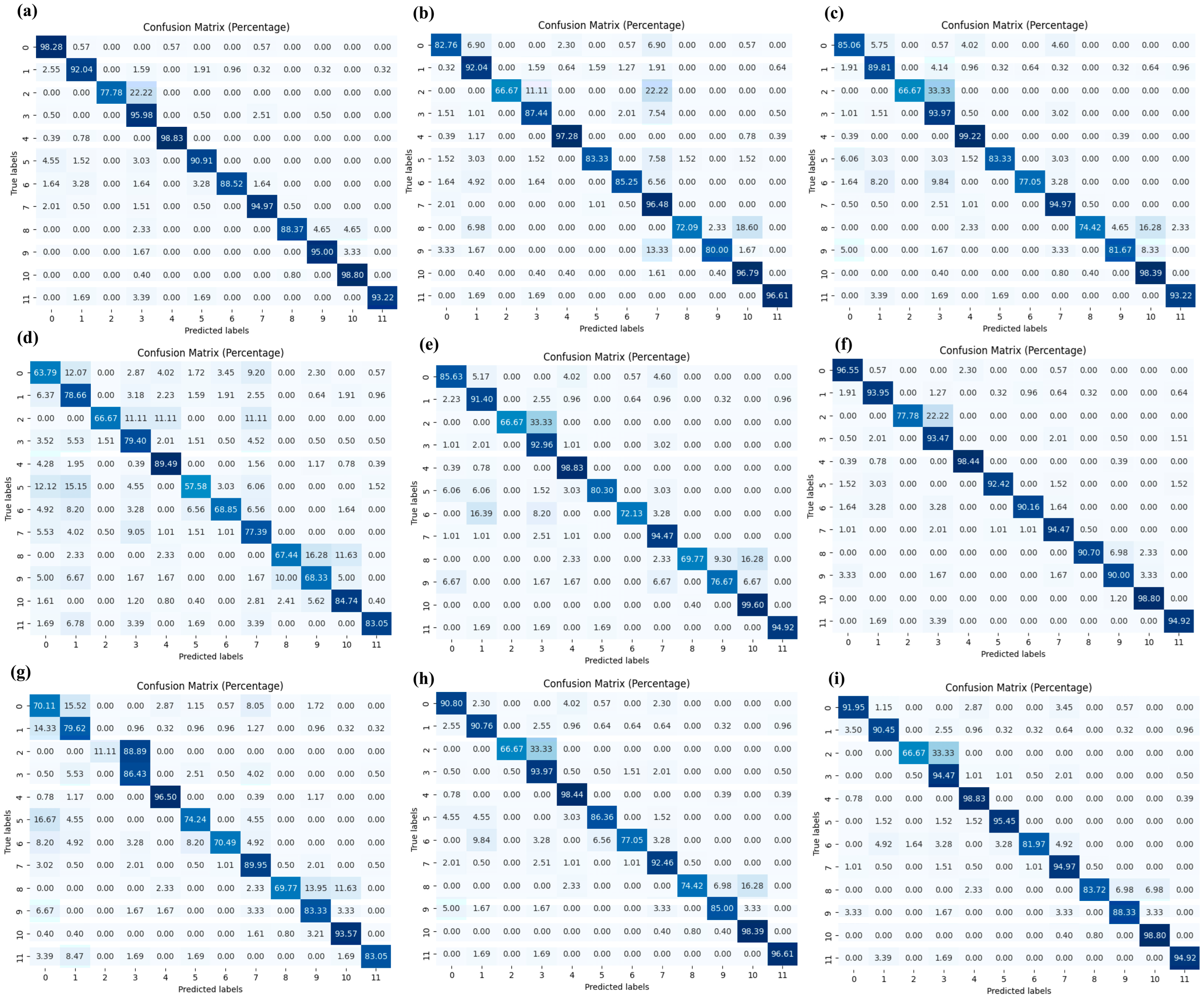
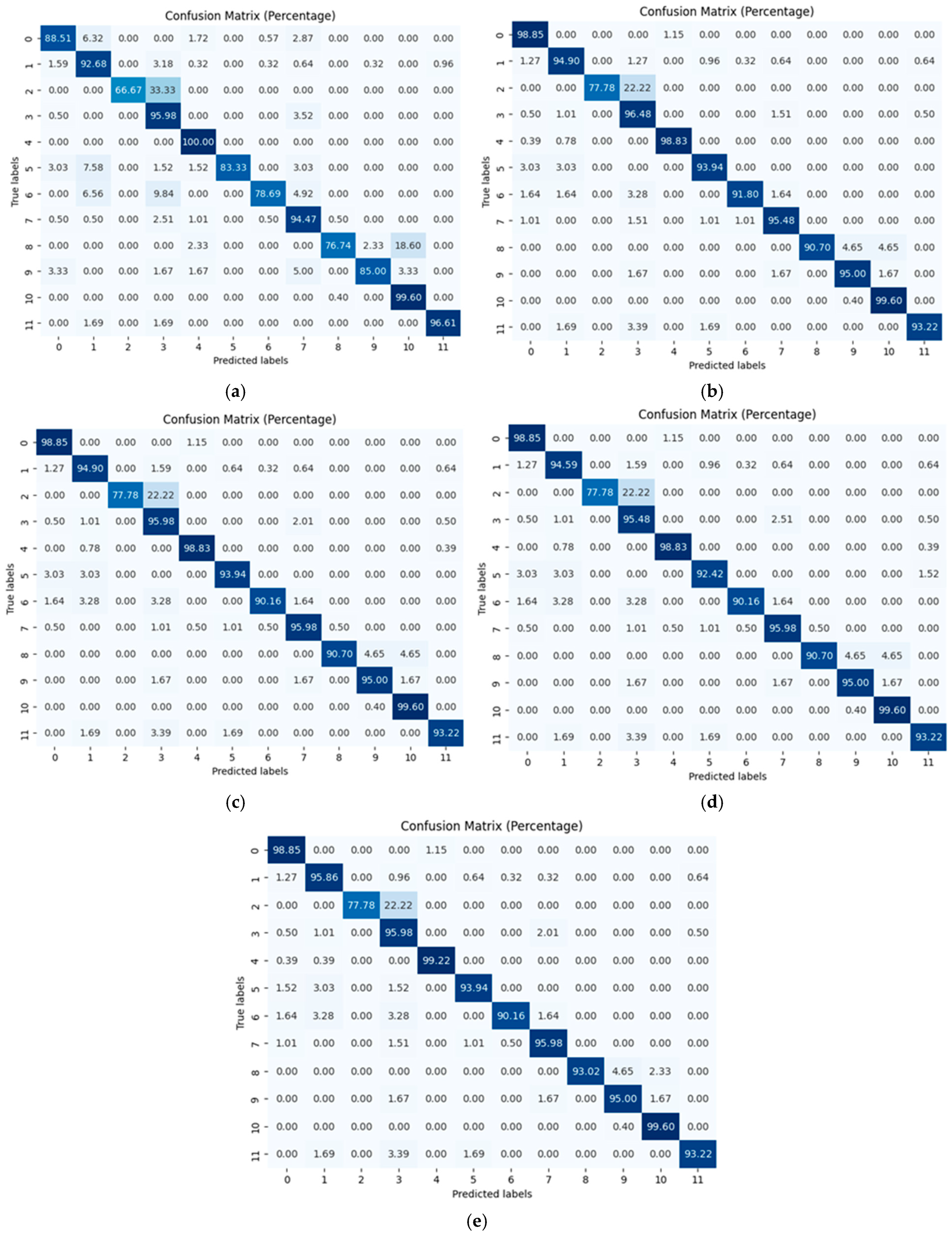
The performance of each individual model and EM in classifying multiple lithologies is extracted principally from confusion matrices (CMs). Figure 6 shows the CMs of SVM (a), KNN (b), RF (c), DT (d), Bagging–DT (e), MLP (f), ADB (g), XGB (h), and HistGBT (i). Additionally, Figure 7 shows the CMs of extra trees (j), stacking (k), voting (l), weighting (m), and blending (n). Based on extracted CMs for the used classification method, there are no major misclassifications, with the high values represented by dark blue. The details of performance metrics have been materialized in

Table 1. Accuracy of classification via SVM, kNN, RF, DT, MLP, ADB, XGB, and extra trees for each class from EnMAP hyperspectral data (all metric values are expressed in percentage). Abbreviation: HT, hyperparameter tuning.

	SVM		kNN		RF		DT		MLP		ADB		XGB		ExTrees
Class No (Sign)	UA	PA	UA	PA	UA	PA	UA	PA	UA	PA	UA	PA	UA	PA	UA	PA
Cl-1 (Xoε)	98.28	90.48	82.76	91.72	85.06	89.16	63.79	62.01	96.55	92.31	70.11	61.31	90.8	88.27	88.51	93.33
Cl-2 (XIξ, luXII2)	92.04	97.31	92.04	91.17	89.81	92.46	78.66	78.16	93.95	96.09	79.62	82.24	90.76	94.68	92.68	92.97
Cl-3 (XIIδ2,Xδ)	77.78	100.0	66.67	100.0	66.67	100.0	66.67	60.0	77.78	100	11.11	100	66.67	85.71	66.67	100
Cl-4 (XII2q)	95.98	91.39	87.44	94.57	93.97	85.00	79.40	77.45	93.47	92.54	86.43	90.05	93.97	90.34	95.98	87.61
Cl-5 (XII3γ, XiγM)	98.83	99.61	97.28	97.28	99.22	94.44	89.49	90.20	98.44	98.44	96.5	96.88	98.44	94.05	100	96.62
Cl-6 (XIIIm)	90.91	84.51	83.33	88.71	83.33	96.49	57.58	65.52	92.42	95.31	74.24	74.24	86.36	87.69	83.33	100
Cl-7 (XIIIS1e, XIIIS1cg)	88.52	94.74	85.25	83.87	77.05	95.92	68.85	71.19	90.16	91.67	70.49	86	77.05	87.04	78.69	94.12
Cl-8 (XIIIS2)	94.97	95.94	96.48	77.42	94.97	89.15	77.39	73.33	94.47	94.95	89.95	81.74	92.46	92	94.47	89.52
Cl- 9 (Ad11b)	88.37	92.68	72.09	96.88	74.42	94.12	67.44	70.73	90.7	95.12	69.77	90.91	74.42	91.43	76.74	94.29
Cl-10 (Ad11a)	95.00	93.44	80.00	96.00	81.67	92.45	68.33	56.94	90	87.1	83.33	64.94	85	89.47	85	96.23
Cl-11 (Ad12b)	98.80	98.40	96.79	94.88	98.39	94.59	84.74	92.14	98.8	98.8	93.57	96.28	98.39	96.46	99.6	96.12
Cl-12 (q2e,q3-4)	93.22	98.21	96.61	93.44	93.22	93.22	83.05	85.96	94.92	90.32	83.05	94.23	96.61	91.94	96.61	95
OA	95.33		91.07		91.72		77.87		95.15		84.38		92.43		93.43
AA	92.73		86.39		86.48		73.78		92.64		75.68		87.58		88.19
Kappa	94.67		89.78		90.52		74.76		94.46		82.17		91.35		92.49
Recall Score	95.33		91.07		91.72		77.87		95.15		84.38		92.43		93.43
F1-Score	95.33		91.06		91.61		77.98		95.15		84.41		92.35		93.34
HT Time (s)	272.317		75.5883		1241.85		58.2372		659.843		1322.95		2563.07		158.265
Training Time (s)	1.0219		0.0013		3.3784		0.3655		4.6161		27.5388		5.711		1.0347

and

Table 2. Accuracy of classification via the EL of Bagging–DT, Boosting–HGB, stacking, voting, weighting, and blending for each class from the EnMAP hyperspectral data.

	Bagging–DT		Boosting–HGB		Stacking		Voting		Weighting		Blending
Class No (Sign)	UA	PA	UA	PA	UA	PA	UA	PA	UA	PA	UA	PA
Cl-1 (Xoε)	85.63	88.17	91.95	90.40	98.85	93.99	98.85	95.03	98.85	95.03	98.85	94.51
Cl-2 (XIξ, luXII2)	91.40	89.97	90.45	96.93	94.90	97.39	94.90	97.07	94.59	97.06	95.86	97.41
Cl-3 (XIIδ2,Xδ)	66.67	100.0	66.67	75.00	77.78	100.0	77.78	100.0	77.78	100.0	77.78	100.0
Cl-4 (XII2q)	92.96	88.52	94.47	90.82	96.48	93.20	95.98	93.17	95.48	93.14	95.98	93.17
Cl-5 (XII3γ, XiγM)	98.83	93.38	98.83	95.13	98.83	99.22	98.83	98.83	98.83	98.83	99.22	99.22
Cl-6 (XIIIm)	80.30	98.15	95.45	92.65	93.94	91.18	93.94	92.54	92.42	91.04	93.94	92.54
Cl-7 (XIIIS1e, XIIIS1cg)	72.13	93.62	81.97	92.59	91.80	94.92	90.16	96.49	90.16	96.49	90.16	96.49
Cl-8 (XIIIS2)	94.47	87.85	94.97	91.30	95.48	96.45	95.98	95.98	95.98	95.50	95.98	96.46
Cl- 9 (Ad11b)	69.77	96.77	83.72	92.31	90.70	100.0	90.70	97.50	90.70	97.50	93.02	100.0
Cl-10 (Ad11a)	76.67	90.20	88.33	91.38	95.00	95.00	95.00	95.00	95.00	95.00	95.00	95.00
Cl-11 (Ad12b)	99.60	95.75	98.80	98.01	99.60	98.80	99.60	98.80	99.60	98.80	99.60	99.20
Cl-12 (q2e,q3-4)	94.92	94.92	94.92	91.80	93.22	94.83	93.22	93.22	93.22	91.67	93.22	94.83
OA	91.48		93.79		96.45		96.39		96.21		96.69
AA	85.28		90.04		93.88		93.75		93.55		94.05
Kappa	90.24		92.91		95.95		95.88		95.68		96.22
Recall Score	91.48		93.79		96.45		96.39		96.21		96.69
F1-Score	91.32		93.75		96.44		96.38		96.20		96.68
HT Time (s)	1078.62		1665.51		2249.6		2249.6		2249.6		2249.6
Training Time (s)	9.9043		7.0604		64.3961		13.8811		55.4483		9.7907

, as well as Figure 8.

Figure 6. Confusion matrices for the various multiclass lithological classification models are presented, including (a) SVM, (b) KNN, (c) RF, (d) DT, (e) Bagging–DT, (f) MLP, (g) ADB, (h) XGB, and (i) HistGBT. These matrices, expressed in percentages, illustrate the performance of each individual model, as well as that of the ensemble method (EM) in classifying multiple lithological units. They enable a comparison of how effectively each model discriminates between different lithologies and highlight misclassifications across the employed classifiers.

Figure 6. Confusion matrices for the various multiclass lithological classification models are presented, including (a) SVM, (b) KNN, (c) RF, (d) DT, (e) Bagging–DT, (f) MLP, (g) ADB, (h) XGB, and (i) HistGBT. These matrices, expressed in percentages, illustrate the performance of each individual model, as well as that of the ensemble method (EM) in classifying multiple lithological units. They enable a comparison of how effectively each model discriminates between different lithologies and highlight misclassifications across the employed classifiers.

Figure 7. Confusion matrices for (a) extra trees, (b) stacking, (c) voting, (d) weighting, and (e) blending. These matrices, expressed in percentages, illustrate the performance of each individual model, as well as that of the ensemble method (EM) in classifying multiple lithological units. They enable a comparison of how effectively each model discriminates between different lithologies and highlight misclassifications across the employed classifiers.

Figure 7. Confusion matrices for (a) extra trees, (b) stacking, (c) voting, (d) weighting, and (e) blending. These matrices, expressed in percentages, illustrate the performance of each individual model, as well as that of the ensemble method (EM) in classifying multiple lithological units. They enable a comparison of how effectively each model discriminates between different lithologies and highlight misclassifications across the employed classifiers.

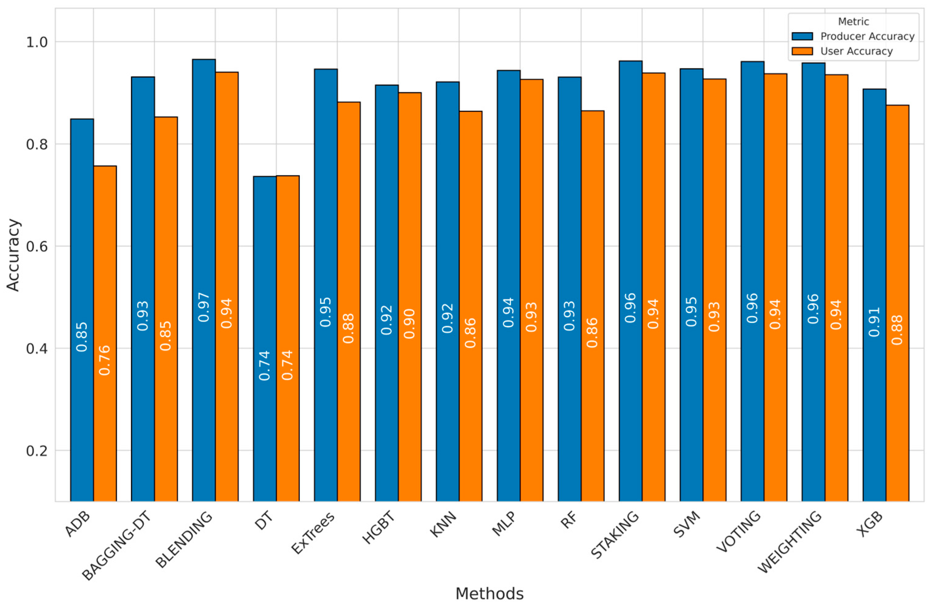
Figure 8. User accuracy (UA) and producer accuracy (PA) are calculated for each classification method for a comparative evaluation of performance across the various algorithms used, whereas EL techniques highlight consistency in handling both omission and commission errors [68].

Figure 8. User accuracy (UA) and producer accuracy (PA) are calculated for each classification method for a comparative evaluation of performance across the various algorithms used, whereas EL techniques highlight consistency in handling both omission and commission errors [68].

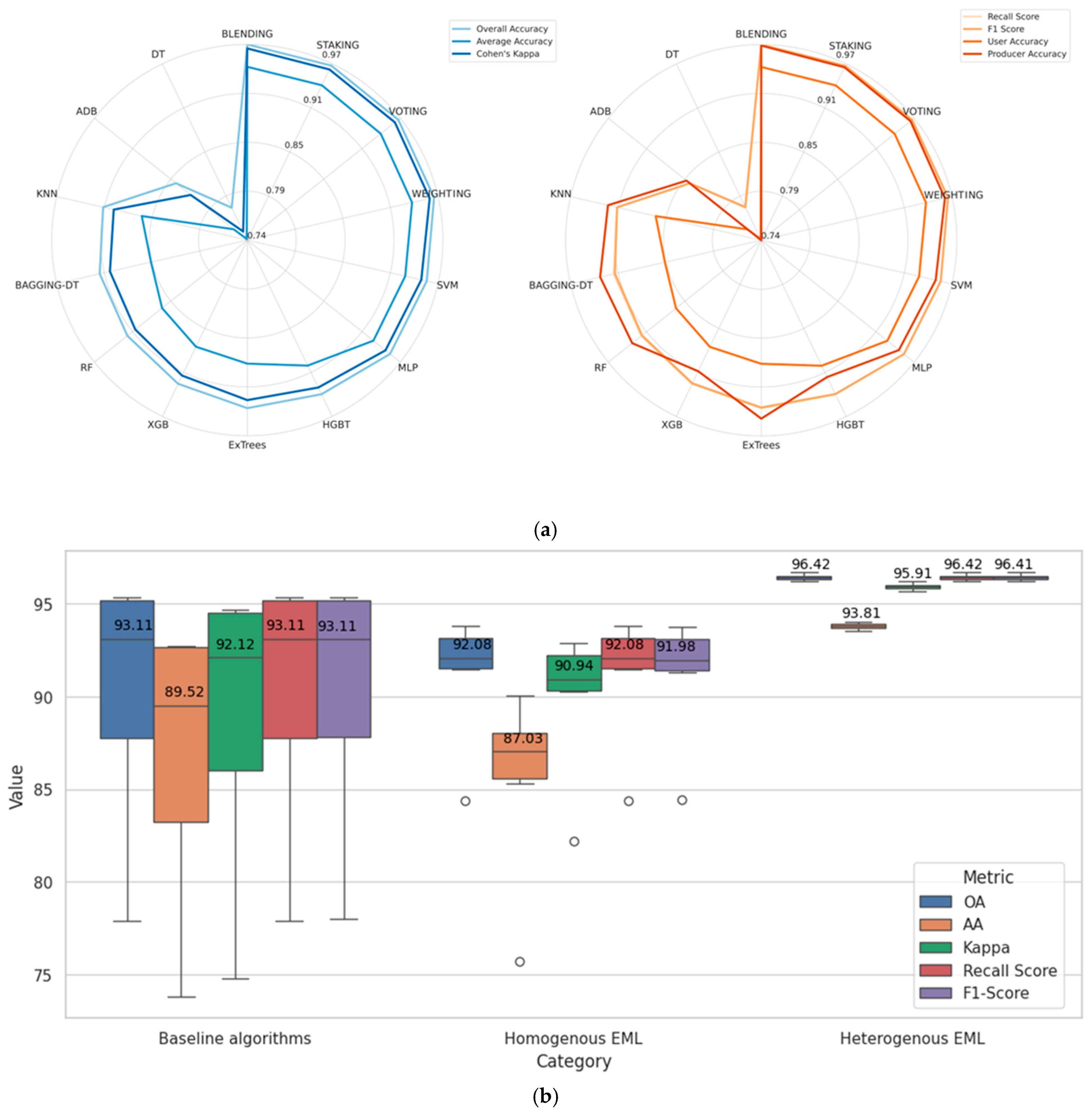
A clear hierarchy of classification the models’ performance based on OA, F1 score, recall, AA, and KA are displayed in Table 1 and Table 2. Blending (0.9669), stacking (0.9645), voting (0.9639), and weighting (0.9621), achieve the highest overall accuracies (Table 2), closely followed by models such as SVM (0.9533) and MLP (0.9515). In contrast, the DT demonstrates the lowest accuracy (0.7787), highlighting the significant advantage of more advanced techniques. Using the five metrics, the ranking of performance is as follows: blending > stacking > voting > weighting > SVM > MLP > HistGBT > extra trees > XGBoost > RF > Bagging–DT > KNN >ADB > DT. Some variations are observed in AA, where KNN slightly outperformed the Bagging–DT model, while the previous order is consistent across the five metrics. The findings from the overall accuracy analysis are further supported by this constant pattern across metrics such as the F1 score, recall, average accuracy, and kappa coefficient, offering a thorough evaluation of the models’ capabilities.

Figure 8 shows a comparative analysis of ensemble models for lithological classification based in UA and PA performance metrics. UA, also known as Pr, reflects prediction precision, while PA, also known as recall, reflects classification completeness. A common trend observed is that Bagging–DT, extra trees, KNN, and RF show a higher PA than UA, suggesting that these models are effective at capturing a large portion of the actual pixels for a class but may suffer from some over-classification or commission errors (Figure 8). Models including blending, stacking, voting, and weighting demonstrate superior performance, with PA exceeding 0.95 and UA surpassing 0.93, indicating a strong ability to both capture actual lithological classes and reliably classify lithological units (Figure 8). Conversely, the decision tree exhibits the lowest PA and UA, both around 0.73, illustrating the significant advantage of ensemble methods, especially where the Bagging–DT has improved the baseline DT model (Figure 8). In contrast, ADB presents a unique profile, with a lower PA (0.7568) but a higher UA (0.8490), indicating a more conservative approach that prioritizes accuracy over comprehensive coverage. The data from Figure 8 underscores the effectiveness of ensemble techniques, with blending, stacking, voting, and weighting achieving a balanced performance by maximizing both PA and UA (Figure 8).

Figure 9b effectively visualizes the relative performance of each model across multiple metrics, making it easy to identify trends and outliers. It is a visually intuitive comparison of the classification models, reinforcing the findings that ensemble methods and advanced algorithms generally offer superior performance in this context. The high performance of blending (OA = 96.69%), stacking (OA = 96.45%), voting (OA = 96.39%), and weighting (OA = 96.21%) underscores the effectiveness of combining multiple heterogeneous ML models for improved lithological classification accuracy. Figure 9b highlights an improvement in the seven metrics values using the last four EL models compared to the rest of the evaluated models. Figure 9b shows the medians of the models used via several performance metrics. The heterogeneous EL models allowed us to obtain optimal results, showing better stability across the four models used and increased OA by 4.34%.

4.2. Training Time

For practical ML deployment, beyond classification accuracy, computational efficiency is critical (Table 1). In this investigation, the execution duration for each algorithm was systematically recorded by programmatically leveraging Python’s module. The results highlight both individual classifiers (e.g., SVM, RF, and XGBoost) and heterogeneous ensemble strategies (stacking, voting, blending, and weighting), offering a comprehensive view of their computational demands and predictive capabilities. Since EL methods integrate multiple base classifiers, the hyperparameter tuning time reflects the sum of their tuning times. In our case, the heterogeneous ensemble (via SVM-KNN-RF-MLP) led to a cumulative tuning time of approximately 2249.60 s. This accumulation is expected, as each base learner must undergo independent hyperparameter optimization before contributing to the final ensemble prediction. The current findings show that while heterogeneous EL methods do introduce higher computational costs during training when counting hyperparameter optimization, these costs remain within practical bounds for most applications, when compared to those of the commonly used ML models. It is noteworthy that a contrast in training time is demonstrated in baseline models: the RF and ADB models required 3.38 s and 27.54 s, respectively for training, with tuning times exceeding 1000 s. On the other hand, simpler models such as KNN and DT were trained extremely quickly (0.0013 s and 0.3655 s, respectively), though at the expense of lower predictive performance, as detailed in the manuscript. On the other hand, the benchmark on the heterogeneous EL models demonstrated that blending emerges as the most efficient heterogeneous ensemble (9.79 s training time), while achieving the highest accuracy, outperforming stacking (64.40 s) and voting (13.88 s). In addition, blending models employ a leave-one-out strategy to construct the meta-feature dataset, which is computationally more efficient and faster. In this realm, and despite the relative higher computational cost of heterogeneous EL models, they offer improved classification performance, which may justify their selection and computational overhead in many practical use cases [69].

4.3. Accuracy of Lithological Unit Mapping

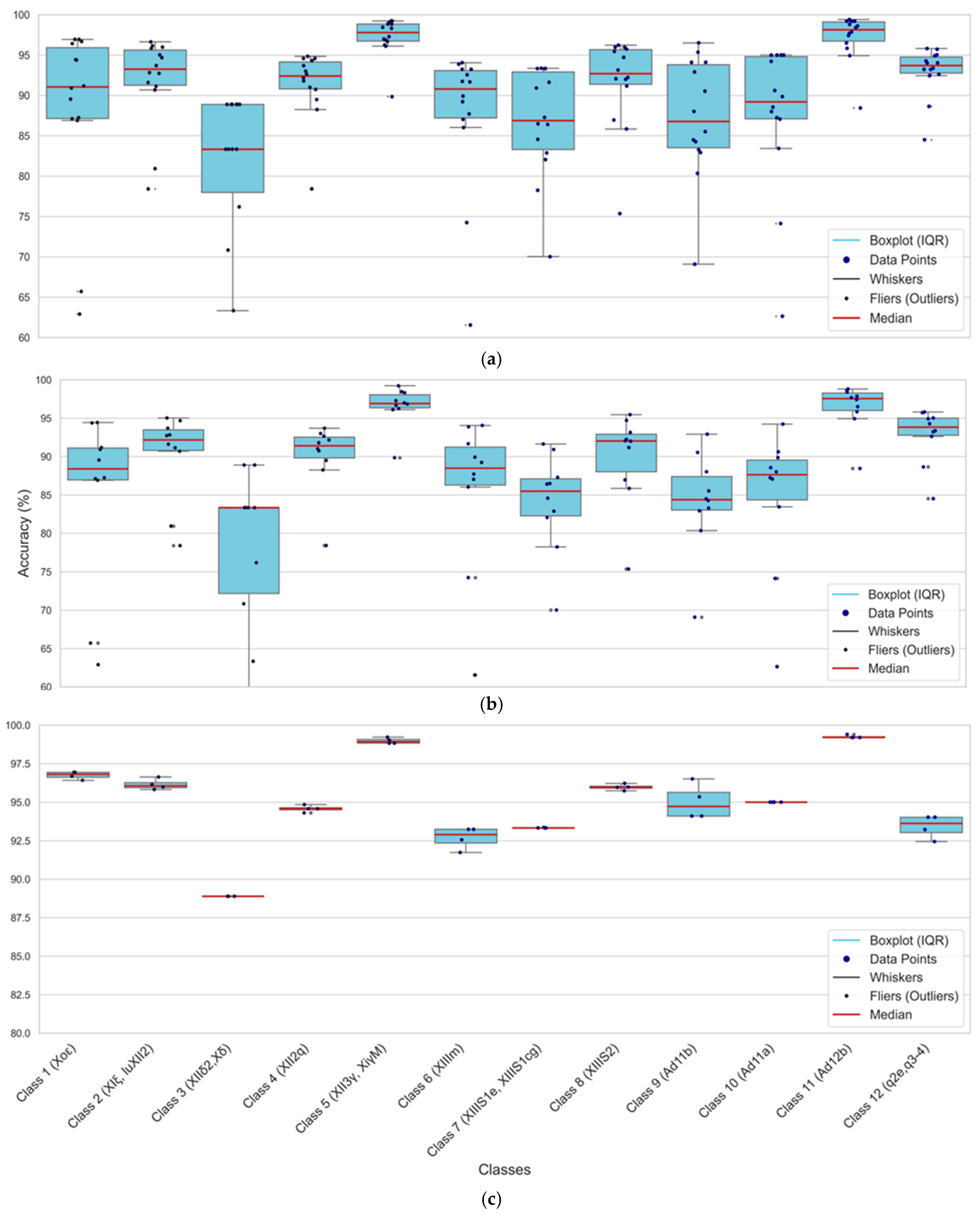
The performance of all the models used, including both baseline and heterogeneous EL models, in classifying the twelve lithological units is clearly detailed in Figure 10. In general, the UA and PA values were averaged for each class, reaffirming that the models trained with the EnMAP data exhibit notable classification capability (see Figure 10a–c). The results highlight the superior performance of all models (Figure 10a), with a median accuracy approaching 90%. The highest accuracy levels were observed for classes 5 and 11, which exhibit exceptionally narrow interquartile ranges (IQRs), indicating high consistency across models. However, omission errors were noted in Class 3 when using base models (Figure 10b).

For most lithological units, a narrow IQR indicates consistent classification performance, while the presence of outliers suggests instances where certain models significantly outperformed others. Among all models, the results of the heterogeneous EL models (Figure 10c) demonstrated the highest accuracy in classifying the twelve lithological unit classes. Additionally, the majority of classes (e.g., 1, 2, 4, 5, 8, 9, 10 and 11) exhibit high median performance, consistently above or near 95%, with narrow IQRs, suggesting stable and reliable classification across the ELEL models used. Classes 3, 6, 7, and 12 exhibit lower median performance, below 93%, with broader IQRs, indicating greater variability and potential challenges in accurate classification. These accuracies have been significantly increased using EL models (Figure 10c), whereas several baseline models (Figure 10b) failed to classify them. These results surpass those achieved by the baseline ML models (Figure 10b) and mitigate the need for testing the performance of several models.

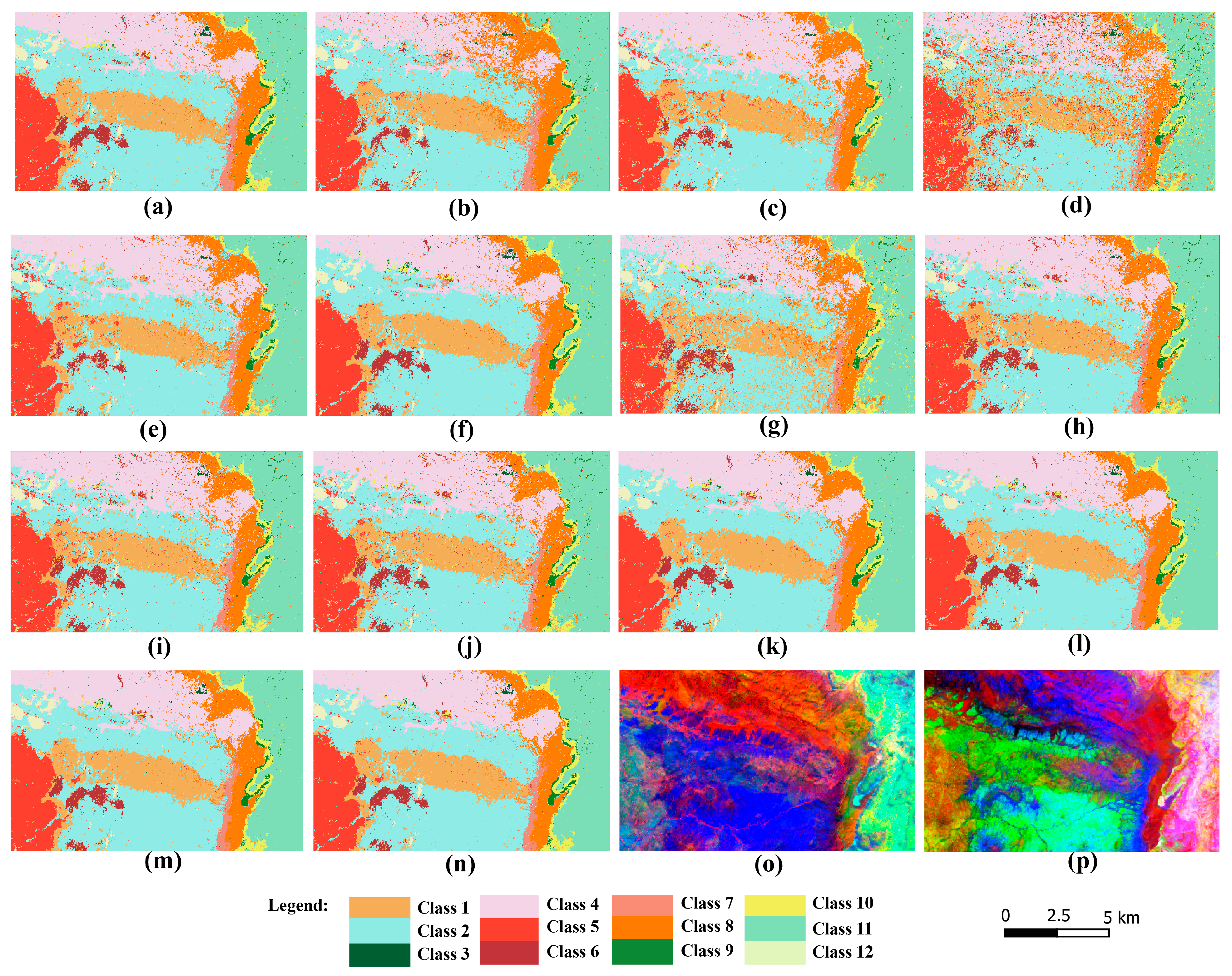
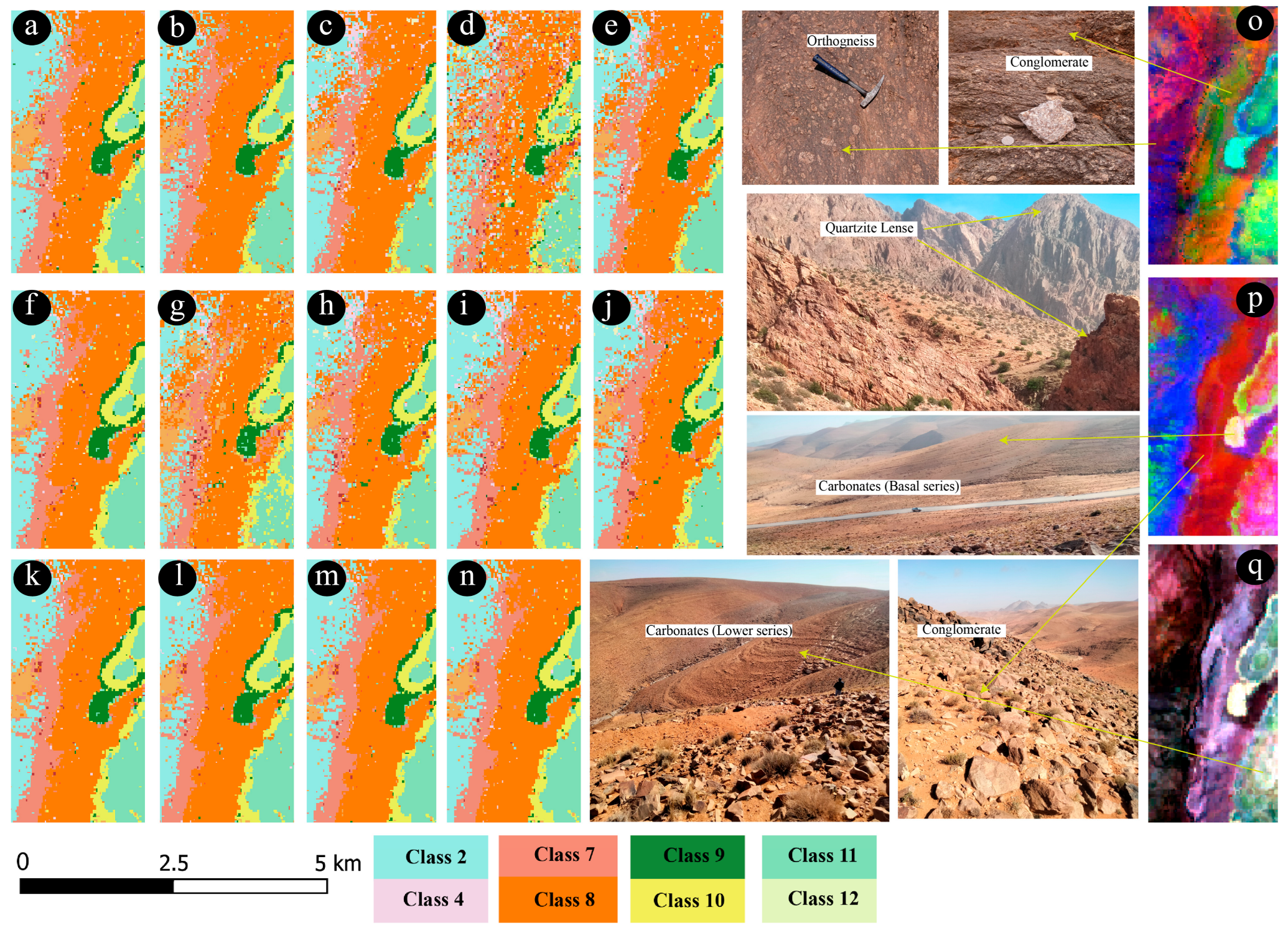
In addition to quantitative accuracy evaluations, visual analyses and comparisons with previously established geological maps were conducted. The final thematic maps underwent validation through on-site geological surveys. Specific observation points were identified and integrated into the final thematic representation using HSI and heterogeneous EL models (Figure 11 and Figure 12). Furthermore, photographs depicting the primary lithological units within the study area are provided in Figure 12, enhancing rock identification and validation. This reinforces the reliability of the proposed approach (heterogeneous EL) for future lithology mapping in analogous geological contexts. Figure 12 also showcases in situ field observations, capturing distinct locations and lithological formations within the investigation area, located around the Idikel mine. The extracted classification maps (Figure 11 and Figure 12) demonstrate substantial potential for aiding the delineation of geological formations within the Eastern Kerdous Inlier and updating previous geological maps.

5. Discussion

5.1. Model Performance Benchmark

Various intelligent modeling approaches have been applied across multiple geoscience domains, providing researchers with valuable insights into lithological compositions [70,71,72,73]. The identification and classification of lithological units have always been a key focus in geological studies [74]. However, current research on the application of EL for lithological mapping based on HSI remains limited. However, several studies have emphasized the potential of non-heterogeneous (e.g., DT, RF, XGB, etc.) ensemble learning in remote sensing applications [75]. A recent study by Giri, Janghel [76] highlighted the effectiveness of a stacked-based heterogeneous (Naïve Bayes, KNN, DT, artificial neural network, and SVM) EL model in mineral mapping using hyperspectral, offering pixel-level valuable insights. They proposed a framework for mineral classification using AVIRIS-NG airborne HSI data over Jahazpur, India, achieving high accuracy (98.96% OA). In addition, by integrating various models, ensemble learning reduces the risk of overfitting, which is a common issue in machine learning [76]. ML models typically require less computational power and can perform effectively with smaller datasets compared to DL models, which often necessitate substantial computational resources and large amounts of labeled data to achieve optimal performance [23]. The comparison of baseline classifiers with ensemble approaches highlights a consistent trend of superior performance with blending, stacking, voting, and weighting, confirming their robustness in hyperspectral lithological mapping. The ranking order of classification models (blending > stacking > voting > weighting > SVM > MLP > HistGBT > extra trees > XGBoost > RF > Bagging–DT > KNN > ADB > DT) suggests that advanced ensemble techniques outperform conventional ML classifiers. The performance of the selected baseline models (SVM, KNN, RF, and MLP), in combination with ensemble learning, further underscores their effectiveness in lithological classification. These classifiers are widely recognized for their ability to capture complex spectral patterns in hyperspectral data [77,78,79], making them ideal candidates for ensemble-based approaches. The DT, on the other hand, exhibited the lowest performance (OA = 77.87%), reinforcing previous findings that DT models tend to suffer from overfitting and high variance [50]. The current study confirms the fact that decision trees are susceptible to producing suboptimal solutions and are prone to overfitting, particularly when dealing with complex or high-dimensional datasets [80]. The current research findings show a 1.4–6% increase in the accuracy of individual baseline classifiers, which is consistent with prior works in hyperspectral data classification in general, where EL outperformed common ML models in various geological settings [23]. In addition, these results corroborate several works, which highlight the fact that combining multiple classifiers reduces uncertainty [81] and enhances classification accuracy [82] in remote sensing applications.

The observed relatively lower performance in certain classes (Figure 10), notably Classes 3, 6, 7, and 12, is often attributable to intrinsic spectral properties, geological context, or spatial representation. Class 3 (dolerites) exhibited persistent poor classification across all maps, which can be attributed to its limited spatial extent within the study area and the influential presence of pyrophyllite alteration minerals, known to significantly impact spectral responses around this unit [38]. Furthermore, the spectral separability between Class 6 and Class 7, both revealing volcanic rocks (based on the geological map of Tafraout), was impacted by the inherent similarities in their spectral–chemical compositions. Class 12, representing Quaternary sediments, naturally displayed a relatively lower accuracy median, since they are formed from the erosion and deposition of diverse surrounding rocks, resulting in spectrally mixed pixels. Despite these specific challenges, it is crucial to note that these classes remained well classified, with their accuracy consistently above 90%, indicating the model’s overall robustness. The consistency in achieving high OA across all classifications (Figure 10c) underscores the effectiveness of the heterogeneous ensemble learning models, demonstrating their superior capability to handle the complexities of the altered and geologically diverse mapped terrain. The consistency of this ranking across multiple metrics (overall accuracy, F1 score, recall, average accuracy, and kappa coefficient) further reinforces the reliability of EL models. This performance contrasts with the EL outputs based on FCCs over the area encompassing the Idikel mine (Figure 12), demonstrating improved delineation of lithological units. Validation was conducted using multiple approaches, including geological point data, spectral signature analysis based on previous observations [38], as well as the interpretation of FCCs as a commonly used technique in remote sensing-based geological mapping [83,84], which confirmed the spectral coherence of the mapped units. Comparing these outputs to existing geological cartography in the region highlights their added value, offering enhanced resolution and accuracy that have important implications for advancing mineral exploration activities.

On the other hand, the superior performance of blending and stacking in this study aligns with previous research, indicating that the ensemble models tend to mitigate overfitting and improve generalization in classification tasks [85]. The results provide strong evidence that ensemble learning significantly enhances classification accuracy in complex geological terrains (Figure 9b). The integration of hyperspectral data with ensemble classifiers has proven effective in identifying lithological units, particularly in hydrothermally altered zones.

5.2. Limitations and Future Directions

While this study substantiates the efficacy of ensemble learning in lithological classification, several important avenues remain for further exploration. First, although the current framework leverages HSI data as the main data set, it does not yet incorporate spectral indices (alteration features), textural features (e.g., GLCM and/or morphological filters), and structural geology insights (e.g., lithological boundaries, structural lineaments, and fracture patterns). Integrating such features could substantially enhance mapping precision and robustness [84,86]. These features could be seamlessly incorporated into the EL framework through multiple strategies, such as feature-level fusion, where they are integrated alongside spectral band inputs. This integration would enrich contextual awareness and likely yield more optimized lithological maps. Accordingly, leveraging geologically meaningful features in this manner would improve the proposed model explainability, contributing to clearer insights into how specific physical characteristics drive mapping outcomes, thereby supporting interpretable and trustworthy results. A notable limitation also stems from the spatial resolution of the EnMAP sensor (~30 m), which constrains the capability to detect and accurately map small geological formations such as narrow dykes or vein systems, potentially leading to underrepresentation of critical mineralized structures, which is already defined during the mapping of doleritic dykes in the study area [6]. Since explainability remains an inherent challenge in EL frameworks, especially as model complexity increases. Future work should consider interpretability by incorporating feature-importance-assessing methods and by evaluating the contributions of individual classifiers within ensemble constructs. This would provide a better understanding of the decision-making process and help geoscientists gain confidence in automated mapping outputs, alongside the current efforts in this realm [84]. These upcoming directions, integrating more intricate predictors, hybridizing proposed EL and DL paradigms, resolving spatial resolution constraints, and deepening model transparency, are indispensable for advancing interpretable and field-deployable solutions for lithological classification and mineral exploration across the AVSZ and comparable geological settings worldwide.

6. Conclusions

In this study, heterogeneous ensemble learning methods such as bagging, boosting, stacking, voting, weighting, and blending were applied and evaluated to overcome the challenges in the accuracy of hyperspectral lithological mapping in the Ameln Valley shear zone in the western Anti-Atlas, Morocco.

Baseline algorithms, homogeneous ensemble models, and heterogeneous ensemble models have been analyzed comparatively in hyperspectral lithological mapping. The results demonstrate that heterogeneous ensemble models achieve the best performance, with high scores and low dispersion across all evaluated metrics, suggesting strong stability and robustness in predictions. In comparison, homogeneous ensemble models show improvement over baseline algorithms but could also exhibit variability due to the influence of weak classifiers. As for baseline algorithms, although they achieve competitive scores on some metrics, they display significant variability with higher dispersion, indicating lower reliability compared to the other classifier groups.

• This study confirms that hyperspectral data, when paired with ensemble learning techniques, is highly effective for lithological mapping in hydrothermally altered complex terrains. The use of ensemble methods, particularly blending, stacking, voting, and weighting, provided valuable improvements in classification accuracy, demonstrating their suitability for mapping the complex geological features of the Ameln Valley.
• The findings suggest that the proposed EL models play a crucial role in enhancing the accurate and efficient HIS-based identification of lithological units, particularly in geologically similar regions. The benchmarking results demonstrate that the blending EL model achieves an impressive OA of 96.96%. This is further highlighted by the ability of other heterogeneous EL models to deliver consistent high and comparable accuracies while maintaining reasonable computational costs when taking into account the combination of multiple models and their lower computational cost compared to DL models, which are known for their relative complexity and for requiring substantial computational power.

This study highlights the effectiveness of ensemble learning techniques, in particular blending, stacking, voting, and weighting, in improving the accuracy of hyperspectral lithological maps in complex mountainous geological regions. The integration of optimized feature subsets and high-dimensional hyperspectral data has proven beneficial and demonstrated the potential of these approaches for detailed lithological analyses in the Ameln Valley region. The results provide valuable insights for future comparative studies, especially for evaluating the capabilities of hyperspectral systems such as EnMAP for lithological mapping in geologically analogue regions. The use of hyperspectral satellite data can significantly improve geological analyses through ensemble learning for sustainable exploration in extreme or data-poor regions. This advancement supports data-driven decision making for mineral exploration in mountainous and remote regions and for monitoring environmental targets.

References

1. Cocks, T.; Jenssen, R.; Stewart, A.; Wilson, I.; Shields, T. The HyMapTM airborne hyperspectral sensor: The system, calibration and performance. In Proceedings of the 1st EARSeL Workshop on Imaging Spectroscopy, Zurich, Switzerland, 6–8 October 1998. [Google Scholar]
2. Bedini, E.; Van Der Meer, F.; Van Ruitenbeek, F. Use of HyMap imaging spectrometer data to map mineralogy in the Rodalquilar caldera, southeast Spain. Int. J. Remote Sens. 2009, 30, 327–348. [Google Scholar] [CrossRef]
3. Tripathi, M.K.; Govil, H. Evaluation of AVIRIS-NG hyperspectral images for mineral identification and mapping. Heliyon 2019, 5, e02931. [Google Scholar] [CrossRef]
4. Adiri, Z.; El Harti, A.; Jellouli, A.; Maacha, L.; Azmi, M.; Zouhair, M.; Bachaoui, E.M. Mapping copper mineralization using EO-1 Hyperion data fusion with Landsat 8 OLI and Sentinel-2A in Moroccan Anti-Atlas. Geocarto Int. 2020, 35, 781–800. [Google Scholar] [CrossRef]
5. Sharma, L.K.; Verma, R.K. AVIRIS-NG hyperspectral data analysis for pre-and post-MNF transformation using per-pixel classification algorithms. Geocarto Int. 2020, 37, 2083–2094. [Google Scholar] [CrossRef]
6. Hajaj, S.; El Harti, A.; Pour, A.B.; Khandouch, Y.; Benaouiss, N.; Hashim, M.; Habashi, J.; Almasi, A. Recurrent-spectral convolutional neural networks (RecSpecCNN) architecture for hyperspectral lithological classification optimization. Earth Sci. Inform. 2025, 18, 125. [Google Scholar] [CrossRef]
7. Wang, Z.; Zuo, R. An Evaluation of Convolutional Neural Networks for Lithological Mapping Based on Hyperspectral Images. IEEE J. Sel. Top. Appl. Earth Obs. Remote Sens. 2024, 17, 6414–6425. [Google Scholar] [CrossRef]
8. Yin, J.; Li, N. Ensemble learning models with a Bayesian optimization algorithm for mineral prospectivity mapping. Ore Geol. Rev. 2022, 145, 104916. [Google Scholar] [CrossRef]
9. Garini, S.A.; Shiddiqi, A.M.; Utama, W.; Jabar, O.A.; Insani, A.N.F. Enhanced Lithology Classification in Well Log Data Using Ensemble Machine Learning Techniques. In Proceedings of the 2024 IEEE International Conference on Artificial Intelligence and Mechatronics Systems (AIMS), Bandung, Indonesia, 21–23 February 2024; IEEE: New York, NY, USA, 2024. [Google Scholar]
10. Li, C.; Li, F.; Liu, C.; Tang, Z.; Fu, S.; Lin, M.; Lv, X.; Liu, S.; Liu, Y. Deep learning-based geological map generation using geological routes. Remote Sens. Environ. 2024, 309, 114214. [Google Scholar] [CrossRef]
11. Liu, J.; Guo, H.; He, Y.; Li, H. Vision Transformer-Based Ensemble Learning for Hyperspectral Image Classification. Remote Sens. 2023, 15, 5208. [Google Scholar] [CrossRef]
12. Karimzadeh, S.; Tangestani, M.H. Evaluating the VNIR-SWIR datasets of WorldView-3 for lithological mapping of a metamorphic-igneous terrain using support vector machine algorithm; a case study of Central Iran. Adv. Space Res. 2021, 68, 2421–2440. [Google Scholar] [CrossRef]
13. Shebl, A.; Hissen, M.; Abdelaziz, M.I.; Csámer, Á. Lithological mapping enhancement by integrating Sentinel 2 and gamma-ray data utilizing support vector machine: A case study from Egypt. Int. J. Appl. Earth Obs. Geoinf. 2021, 105, 102619. [Google Scholar] [CrossRef]
14. Shirmard, H.; Farahbakhsh, E.; Heidari, E.; Pour, A.B.; Pradhan, B.; Müller, D.; Chandra, R. A comparative study of convolutional neural networks and conventional machine learning models for lithological mapping using remote sensing data. Remote Sens. 2022, 14, 819. [Google Scholar] [CrossRef]
15. Ge, W.; Cheng, Q.; Tang, Y.; Jing, L.; Gao, C. Lithological classification using sentinel-2A data in the Shibanjing ophiolite complex in inner Mongolia, China. Remote Sens. 2018, 10, 638. [Google Scholar] [CrossRef]
16. Jia, X.; Kuo, B.-C.; Crawford, M.M. Feature mining for hyperspectral image classification. Proc. IEEE 2013, 101, 676–697. [Google Scholar] [CrossRef]
17. Ustuner, M. Randomized Principal Component Analysis for Hyperspectral Image Classification. In Proceedings of the 2024 IEEE Mediterranean and Middle-East Geoscience and Remote Sensing Symposium (M2GARSS), Oran, Algeria, 15–17 April 2024; IEEE: New York, NY, USA, 2024. [Google Scholar]
18. Ganaie, M.A.; Hu, M.; Malik, A.K.; Tanveer, M.; Suganthan, P.N. Ensemble deep learning: A review. Eng. Appl. Artif. Intell. 2022, 115, 105151. [Google Scholar] [CrossRef]
19. Majeed, R.; Abdullah, N.A.; Mushtaq, M.F.; Umer, M.; Nappi, M. Intelligent cyber-security system for iot-aided drones using voting classifier. Electronics 2021, 10, 2926. [Google Scholar] [CrossRef]
20. Salman, H.A.; Kalakech, A.; Steiti, A. Random forest algorithm overview. Babylon. J. Mach. Learn. 2024, 2024, 69–79. [Google Scholar] [CrossRef]
21. Heidari, N.; Khaloozadeh, H. Detection of Fault and Cyber Attack in Cyber-Physical System Based on Ensemble Convolutional Neural Network. In Proceedings of the 2024 10th International Conference on Control, Instrumentation and Automation (ICCIA), Kashan, Iran, 5–7 November 2024; IEEE: New York, NY, USA, 2024. [Google Scholar]
22. Wang, H.; Ma, Z.; Qi, W.; Zhang, N.; Zhuang, H. A Research Review of the Stacking Classification Model. In Proceedings of the 2024 6th International Conference on Machine Learning, Big Data and Business Intelligence (MLBDBI), Hangzhou, China, 1–3 November 2024; IEEE: New York, NY, USA, 2024. [Google Scholar]
23. Han, W.; Zhang, X.; Wang, Y.; Wang, L.; Huang, X.; Li, J.; Wang, S.; Chen, W.; Li, X.; Feng, R.; et al. A survey of machine learning and deep learning in remote sensing of geological environment: Challenges, advances, and opportunities. ISPRS J. Photogramm. Remote Sens. 2023, 202, 87–113. [Google Scholar] [CrossRef]
24. Shebl, A.; Abriha, D.; Fahil, A.S.; El-Dokouny, H.A.; Elrasheed, A.A.; Csámer, Á. PRISMA hyperspectral data for lithological mapping in the Egyptian Eastern Desert: Evaluating the support vector machine, random forest, and XG boost machine learning algorithms. Ore Geol. Rev. 2023, 161, 105652. [Google Scholar] [CrossRef]
25. Wang, S.; Zhou, K.; Wang, J.; Zhao, J. Identifying and mapping alteration minerals using HySpex airborne hyperspectral data and random forest algorithm. Front. Earth Sci. 2022, 10, 871529. [Google Scholar] [CrossRef]
26. Cardoso-Fernandes, J.; Teodoro, A.C.; Lima, A.; Roda-Robles, E. Evaluating the performance of support vector machines (SVMs) and random forest (RF) in Li-pegmatite mapping: Preliminary results. In Earth Resources and Environmental Remote Sensing/GIS Applications X; SPIE: Bellingham, DC, USA, 2019. [Google Scholar]
27. Hajaj, S.; El Harti, A.; Jellouli, A.; Pour, A.B.; Himyari, S.M.; Hamzaoui, A.; Hashim, M. Evaluating the Performance of Machine Learning and Deep Learning Techniques to HyMap Imagery for Lithological Mapping in a Semi-Arid Region: Case Study from Western Anti-Atlas, Morocco. Minerals 2023, 13, 766. [Google Scholar] [CrossRef]
28. Lin, N.; Liu, H.; Li, G.; Wu, M.; Li, D.; Jiang, R.; Yang, X. Extraction of mineralized indicator minerals using ensemble learning model optimized by SSA based on hyperspectral image. Open Geosci. 2022, 14, 1444–1465. [Google Scholar] [CrossRef]
29. Farhadi, S.; Tatullo, S.; Konari, M.B.; Afzal, P. Evaluating StackingC and ensemble models for enhanced lithological classification in geological mapping. J. Geochem. Explor. 2024, 260, 107441. [Google Scholar] [CrossRef]
30. Remidi, S.; Boutaleb, A.; Tachi, S.E.; Hasnaoui, Y.; Szczepanek, R.; Seffari, A. Ensemble machine learning model for exploration and targeting of Pb-Zn deposits in Algeria. Earth Sci. Inform. 2025, 18, 226. [Google Scholar] [CrossRef]
31. Faik, F.; Belfoul, M.A.; Bouabdelli, M.; Hassenforder, B. The structures of the Late Neoproterozoic and Early Palæozoic cover of the Tata area, western Anti-Atlas, Morocco: Polyphased deformation or basement/cover interactions during the Variscan orogeny? J. Afr. Earth Sci. 2001, 32, 765–776. [Google Scholar] [CrossRef]
32. Gasquet, D.; Levresse, G.; Cheilletz, A.; Azizi-Samir, M.R.; Mouttaqi, A. Contribution to a geodynamic reconstruction of the Anti-Atlas (Morocco) during Pan-African times with the emphasis on inversion tectonics and metallogenic activity at the Precambrian–Cambrian transition. Precambrian Res. 2005, 140, 157–182. [Google Scholar] [CrossRef]
33. Hassenforder, B. La Tectonique Panafricaine et Varisque de L’Anti-Atlas Dans le Massif du Kerdous (Maroc); Université Louis Pasteur: Strasbourg, France, 1987; p. 249. [Google Scholar]
34. Benssaou, M.; Hamoumi, N. The western Anti-Atlas of Morocco: Sedimentological and palaeogeographical formation studies in the Early Cambrian. J. Afr. Earth Sci. 2001, 32, 351–372. [Google Scholar] [CrossRef]
35. Hajaj, S.; El Harti, A.; Jellouli, A.; Pour, A.B.; Himyari, S.M.; Hamzaoui, A.; Bensalah, M.K.; Benaouiss, N.; Hashim, M. HyMap imagery for copper and manganese prospecting in the east of Ameln valley shear zone (Kerdous inlier, western Anti-Atlas, Morocco). J. Spat. Sci. 2023, 69, 81–102. [Google Scholar] [CrossRef]
36. Choubert, G.; Faure-Muret, A. The Precambrian Iron and Manganese Deposits of the Anti-Atlas. 1973. Available online: https://unesdoc.unesco.org/ark:/48223/pf0000007174 (accessed on 1 January 2021).
37. Gasquet, D.; Ennih, N.; Liégeois, J.-P.; Soulaimani, A. The Pan-African Belt. In Continental Evolution: The Geology of Morocco; Springer: Berlin/Heidelberg, Germany, 2008; pp. 33–64. [Google Scholar]
38. Hajaj, S.; El Harti, A.; Jellouli, A.; Pour, A.B.; Himyari, S.M.; Hamzaoui, A.; Bensalah, M.K.; Benaouis, N.; Hashim, M. HyMap airborne imaging spectroscopy for mineral potential mapping of cupriferous mineralization in a semi-arid region based on pixel/sub-pixel hydrothermal alteration minerals mapping–A case study. In Proceedings of the Copernicus Meetings, Vienna, Austria, 24–28 April 2023. [Google Scholar]
39. Jellouli, A.; Chakouri, M.; Adiri, Z.; EL Hachimi, J.; Jari, A. Lithological and hydrothermal alteration mapping using Terra ASTER and Landsat-8 OLI multispectral data in the north-eastern border of Kerdous inlier, western Anti-Atlasic belt, Morocco. Artif. Satell. J. Planet. Geod. 2025, 60, 14–36. [Google Scholar] [CrossRef]
40. Chabrillat, S.; Segl, K.; Foerster, S.; Brell, M.; Guanter, L.; Schickling, A. EnMAP Pre-Launch and Start Phase: Mission Update. In Proceedings of the IGARSS 2022-2022 IEEE International Geoscience and Remote Sensing Symposium, Kuala Lumpur, Malaysia, 17–22 July 2022; IEEE: New York, NY, USA, 2022. [Google Scholar]
41. Chabrillat, S.; Guanter, L.; Kaufmann, H.; Foerster, S.; Beamish, A.; Brosinsky, A.; Wulf, H.; Asadzadeh, S.; Bochow, M.; Bohn, N.; et al. EnMAP Science Plan. 2022. Available online: https://www.enmap.org/data/doc/Science_Plan_EnMAP_2022_final.pdf (accessed on 2 February 2023).
42. Kaufmann, H.; Segl, K.; Itzerott, S.; Bach, H.; Wagner, A.; Hill, J.; Heim, B.; Oppermann, K.; Heldens, W.; Stein, E.; et al. Hyperspectral Algorithms: Report in the Frame of EnMAP Preparation Activities. 2010. Available online: https://www.researchgate.net/publication/224992289_Hyperspectral_Algorithms_Report_in_the_frame_of_EnMAP_preparation_activities (accessed on 1 January 2021).
43. Cortes, C.; Vapnik, V. Support-vector networks. Mach. Learn. 1995, 20, 273–297. [Google Scholar] [CrossRef]
44. Cover, T.; Hart, P. Nearest neighbor pattern classification. IEEE Trans. Inf. Theory 1967, 13, 21–27. [Google Scholar] [CrossRef]
45. Rosenblatt, F. The perceptron: A probabilistic model for information storage and organization in the brain. Psychol. Rev. 1958, 65, 386. [Google Scholar] [CrossRef]
46. Apicella, A.; Donnarumma, F.; Isgrò, F.; Prevete, R. A survey on modern trainable activation functions. Neural Netw. 2021, 138, 14–32. [Google Scholar] [CrossRef] [PubMed]
47. Quinlan, J.R. Induction of decision trees. Mach. Learn. 1986, 1, 81–106. [Google Scholar] [CrossRef]
48. Chern, C.-C.; Chen, Y.-J.; Hsiao, B. Decision tree–based classifier in providing telehealth service. BMC Med. Inform. Decis. Mak. 2019, 19, 104. [Google Scholar] [CrossRef]
49. Breiman, L. Random Forests-Random Features; Technical Report 567; Department of Statistics, University of California: Berkeley, CA, USA, 1999; p. 31. [Google Scholar]
50. Breiman, L. Random forests. Mach. Learn. 2001, 45, 5–32. [Google Scholar] [CrossRef]
51. Rodriguez-Galiano, V.F.; Ghimire, B.; Rogan, J.; Chica-Olmo, M.; Rigol-Sanchez, J.P. An assessment of the effectiveness of a random forest classifier for land-cover classification. ISPRS J. Photogramm. Remote Sens. 2012, 67, 93–104. [Google Scholar] [CrossRef]
52. Pal, M. Random forest classifier for remote sensing classification. Int. J. Remote Sens. 2005, 26, 217–222. [Google Scholar] [CrossRef]
53. Breiman, L. Bagging predictors. Mach. Learn. 1996, 24, 123–140. [Google Scholar] [CrossRef]
54. Geurts, P.; Ernst, D.; Wehenkel, L. Extremely randomized trees. Mach. Learn. 2006, 63, 3–42. [Google Scholar] [CrossRef]
55. Elith, J.; Leathwick, J.R.; Hastie, T. A working guide to boosted regression trees. J. Anim. Ecol. 2008, 77, 802–813. [Google Scholar] [CrossRef] [PubMed]
56. Freund, Y.; Schapire, R.E. A decision-theoretic generalization of on-line learning and an application to boosting. J. Comput. Syst. Sci. 1997, 55, 119–139. [Google Scholar] [CrossRef]
57. Chen, T.; Guestrin, C. Xgboost: A scalable tree boosting system. In Proceedings of the 22nd Acm Sigkdd International Conference on Knowledge Discovery and Data Mining, San Francisco, CA, USA, 13–17 August 2016. [Google Scholar]
58. Cui, J.; Hang, H.; Wang, Y.; Lin, Z. GBHT: Gradient boosting histogram transform for density estimation. In Proceedings of the International Conference on Machine Learning, Online, 18–24 July 2021. [Google Scholar]
59. Goumghar, L.; Hajaj, S.; Haida, S.; Kili, M.; Mridekh, A.; Khandouch, Y.; Jari, A.; El Harti, A.; El Mansouri, B. Analysis of Baseline and Novel Boosting Models for Flood-Prone Prediction and Explainability: Case from the Upper Drâa Basin (Morocco). Earth 2025, 6, 69. [Google Scholar] [CrossRef]
60. Nhat-Duc, H.; Van-Duc, T. Comparison of histogram-based gradient boosting classification machine, random Forest, and deep convolutional neural network for pavement raveling severity classification. Autom. Constr. 2023, 148, 104767. [Google Scholar] [CrossRef]
61. Xu, Q.; Yordanov, V.; Amici, L.; Brovelli, M.A. Landslide susceptibility mapping using ensemble machine learning methods: A case study in Lombardy, Northern Italy. Int. J. Digit. Earth 2024, 17, 2346263. [Google Scholar] [CrossRef]
62. Wolpert, D.H. Stacked generalization. Neural Netw. 1992, 5, 241–259. [Google Scholar] [CrossRef]
63. Li, H.; Wang, Y.; Wang, H.; Zhou, B. Multi-window based ensemble learning for classification of imbalanced streaming data. World Wide Web 2017, 20, 1507–1525. [Google Scholar] [CrossRef]
64. Töscher, A.; Jahrer, M.; Bell, R.M. The bigchaos solution to the netflix grand prize. Netflix Prize. Doc. 2009, 1–52. [Google Scholar]
65. Bergstra, J.; Bengio, Y. Random search for hyper-parameter optimization. J. Mach. Learn. Res. 2012, 13, 281–305. [Google Scholar]
66. Claesen, M.; De Moor, B. Hyperparameter search in machine learning. arXiv 2015, arXiv:1502.02127. [Google Scholar] [CrossRef]
67. Probst, P.; Wright, M.N.; Boulesteix, A.L. Hyperparameters and tuning strategies for random forest. Wiley Interdiscip. Rev. Data Min. Knowl. Discov. 2019, 9, e1301. [Google Scholar] [CrossRef]
68. Story, M.; Congalton, R.G. Accuracy assessment: A user’s perspective. Photogramm. Eng. Remote Sens. 1986, 52, 397–399. [Google Scholar]
69. Sulaiman, R.; Azeman, N.H.; Mokhtar, M.H.H.; Mobarak, N.N.; Abu Bakar, M.H.; Bakar, A.A.A. Hybrid ensemble-based machine learning model for predicting phosphorus concentrations in hydroponic solution. Spectrochim. Acta Part A Mol. Biomol. Spectrosc. 2024, 304, 123327. [Google Scholar] [CrossRef]
70. Gupta, R.P. Remote Sensing Geology; Springer: Berlin/Heidelberg, Germany, 2017. [Google Scholar]
71. Hajaj, S.; El Harti, A.; Pour, A.B.; Jellouli, A.; Adiri, Z.; Hashim, M. A review on hyperspectral imagery application for lithological mapping and mineral prospecting: Machine learning techniques and future prospects. Remote Sens. Appl. Soc. Environ. 2024, 35, 101218. [Google Scholar] [CrossRef]
72. Shirmard, H.; Farahbakhsh, E.; Müller, R.D.; Chandra, R. A review of machine learning in processing remote sensing data for mineral exploration. Remote Sens. Environ. 2022, 268, 112750. [Google Scholar] [CrossRef]
73. Sabins, F.F. Remote sensing for mineral exploration. Ore Geol. Rev. 1999, 14, 157–183. [Google Scholar] [CrossRef]
74. Peyghambari, S.; Zhang, Y. Hyperspectral remote sensing in lithological mapping, mineral exploration, and environmental geology: An updated review. J. Appl. Remote Sens. 2021, 15, 031501. [Google Scholar] [CrossRef]
75. Belgiu, M.; Drăguţ, L. Random forest in remote sensing: A review of applications and future directions. ISPRS J. Photogramm. Remote Sens. 2016, 114, 24–31. [Google Scholar] [CrossRef]
76. Giri, R.N.; Janghel, R.R.; Govil, H.; Mishra, G. A stacked ensemble learning-based framework for mineral mapping using AVIRIS-NG hyperspectral image. J. Earth Syst. Sci. 2024, 133, 107. [Google Scholar] [CrossRef]
77. Li, H.; Cui, J.; Zhang, X.; Han, Y.; Cao, L. Dimensionality reduction and classification of hyperspectral remote sensing image feature extraction. Remote Sens. 2022, 14, 4579. [Google Scholar] [CrossRef]
78. Hajaj, S.; El Harti, A.; Pour, A.B.; Khandouch, Y.; Üstüner, M.; Amiri, M.M. Balancing Hyperspectral Dimensionality Reduction and Information Preservation for Machine Learning-based Lithological Classification using EnMAP hyperspectral imagery. Remote Sens. Appl. Soc. Environ. 2025, 38, 101618. [Google Scholar] [CrossRef]
79. Grewal, R.; Singh Kasana, S.; Kasana, G. Machine learning and deep learning techniques for spectral spatial classification of hyperspectral images: A comprehensive survey. Electronics 2023, 12, 488. [Google Scholar] [CrossRef]
80. Maxwell, A.E.; Warner, T.A.; Fang, F. Implementation of machine-learning classification in remote sensing: An applied review. Int. J. Remote Sens. 2018, 39, 2784–2817. [Google Scholar] [CrossRef]
81. Khatami, R.; Mountrakis, G.; Stehman, S.V. A meta-analysis of remote sensing research on supervised pixel-based land-cover image classification processes: General guidelines for practitioners and future research. Remote Sens. Environ. 2016, 177, 89–100. [Google Scholar] [CrossRef]
82. Du, P.; Xia, J.; Zhang, W.; Tan, K.; Liu, Y.; Liu, S. Multiple classifier system for remote sensing image classification: A review. Sensors 2012, 12, 4764–4792. [Google Scholar] [CrossRef] [PubMed]
83. Ghoneim, S.M.; Hamimi, Z.; Abdelrahman, K.; Khalifa, M.A.; Shabban, M.; Abdelmaksoud, A.S. Machine learning and remote sensing-based lithological mapping of the Duwi Shear-Belt area, Central Eastern Desert, Egypt. Sci. Rep. 2024, 14, 17010. [Google Scholar] [CrossRef]
84. Zhang, T.; Zhao, Z.; Dong, P.; Tang, B.-H.; Zhang, G.; Feng, L.; Zhang, X. Rapid lithological mapping using multi-source remote sensing data fusion and automatic sample generation strategy. Int. J. Digit. Earth 2024, 17, 2420824. [Google Scholar] [CrossRef]
85. Njoku, A.O.; Mpinda, B.N.; Awe, O.O. Enhancing Predictive Performance Through Optimized Ensemble Stacking for Imbalanced Classification Problems, in Practical Statistical Learning and Data Science Methods: Case Studies from LISA 2020 Global Network, USA; Springer: Berlin/Heidelberg, Germany, 2024; pp. 575–595. [Google Scholar]
86. Portes, L.; Pirot, G.; Nzikou, M.M.; Giraud, J.; Lindsay, M.; Jessell, M.; Cripps, E. Feature fusion-enhanced t-SNE image atlas for geophysical features discovery. Sci. Rep. 2025, 15, 17152. [Google Scholar] [CrossRef]
Figure 3. Diagram showing the voting EL method.
Minerals 15 00833 g003
Figure 4. Stacking and blending EL methods.
Minerals 15 00833 g004
Figure 5. Weighted EL method.
Minerals 15 00833 g005
Figure 9. Representation of performance metrics for machine learning models, comparing all single and ensemble learning models used (a). The performance variations are highlighted in the baseline model, and the homogeneous EL models, as well as the median, are calculated for each category of models (b). The boxplot visualizes the distribution of model performance metrics: the central line represents the median, the box spans the interquartile range (IQR), and the whiskers extend to 1.5 × IQR. Outliers are shown as individual points, which are particularly evident when using homogeneous EL models.
Minerals 15 00833 g009
Figure 10. Accuracy values of each class, obtained by averaging UA and PA: (a) shows the extracted values using the fourteen models; (b) represents the extracted values from baseline models; (c) represents the extracted results from EL bagging, boosting, stacking, weighting, and blending, where higher consistency, as well as accuracies, is observed for all the mapped twelve lithological units. The presence of outlines (filters) in subfigures (a,b) reflects the greater variability in performance observed with baseline models and homogeneous EL models, emphasizing the contrast with the higher consistency achieved by ensemble methods. On the other hand, (c) supports understanding of the consistency and accuracy achieved across all twelve mapped lithological units, clearly demonstrating the enhanced stability and performance provided by the proposed EL strategies.
Minerals 15 00833 g010
Figure 11. Lithological mapping results: SVM (a), KNN (b), RF (c), DT (d), Bagging–DT (e), MLP (f), ADB (g), XGB (h), HistGBT (i), extra trees (j), stacking (k), voting (l), weighting (m), blending (n). The FCCs as RGB (red, green, and blue) are shown for visual investigation using FCC MNF 3.2.1 (o) and PC3.MNF.2.3 (p).
Minerals 15 00833 g011
Figure 12. Localized false color composites compared to the extracted sub-maps using 14 ML and EL models. Lithological mapping result subsets and FCCs from PCA and MNF: SVM (a), KNN (b), RF (c), DT (d), Bagging–DT (e), MLP (f), ADB (g), XGB (h), HistGBT (i), extra trees (j), stacking (k), voting (l), weighting (m), and blending (n). The subsets of the FCC MNF 3.2.1, PC3.MNF.2.3., and EnMAP 80.184.197 as R.G.B are shown in (o), (p), and (q), respectively.
Minerals 15 00833 g012