Knowledge–Data Collaboration-Driven Mineral Prospectivity Prediction with Graph Attention Networks

Abstract

Predicting mineral deposits accurately requires capturing the complex interactions among geological structures, geochemical anomalies, and alteration patterns. To address this challenge, this study develops a Knowledge–Data Collaboration Graph Attention Network (KDCGAT) to improve copper mineralization prediction by integrating multi-source geological data. The model combines Graph Attention Network (GAT) with multimodal geoscience data, including fracture structures, remote sensing alteration maps, and geochemical anomalies. Spatial correlations are captured through a self-attention mechanism, aligning deep learning predictions with geological and geochemical knowledge. Using the eastern Tien Shan copper belt in Xinjiang as a case study, KDCGAT achieves a copper deposit identification accuracy of 85.9%, outperforming Weight of Evidence (WoE) by 7%, Graph Convolutional Network (GCN) by 11.3%, and Convolutional Neural Network (CNN) by 19.7%. Ablation experiments show a 21.1% improvement over the baseline GAT model. Finally, five Class A and three Class B mineralization prediction zones are delineated. This study demonstrates the effectiveness of graph neural networks for copper prospectivity prediction and highlights knowledge–data collaboration as a practical tool for mineral exploration.

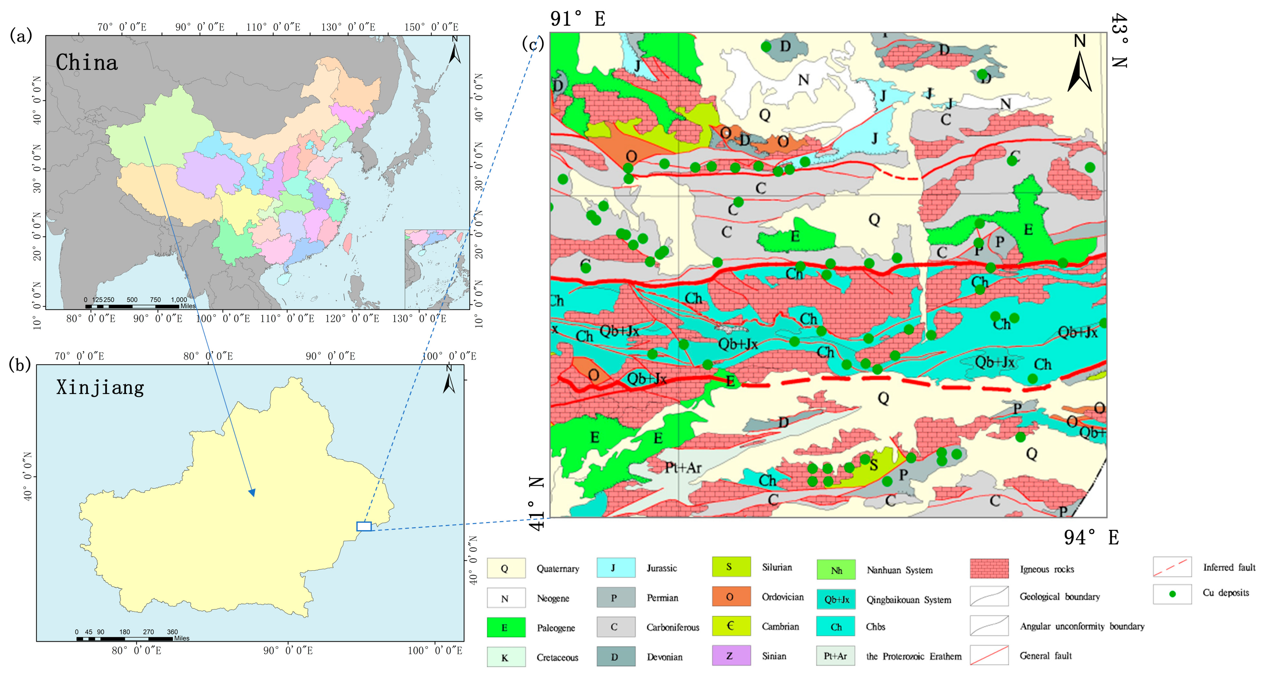
1. Introduction

The exploration and prediction of mineral resources are fundamental tasks in geological science. Their accuracy directly affects the efficiency, economic cost, and environmental sustainability of resource development [1]. With the increasing depletion of shallow mineral deposits, the exploration of concealed ore bodies imposes higher demands on the capacity of prediction models to represent complex geological systems. Therefore, developing high-precision and interpretable intelligent prediction methods has both theoretical significance and practical value. Traditional mineral prospectivity mapping relies largely on experience-driven approaches [2,3], which have significant bottlenecks. The Weight of Evidence (WoE) model, based on Bayesian probability superposition, assumes that ore-forming factors are independent [4,5]. This simplification neglects the nonlinear interactions among faults, alterations, and geochemical anomalies, as well as the dynamic coupling effects of multi-stage tectonic and hydrothermal processes [6]. Consequently, such approaches often yield fragmented or overly smoothed prediction results. Moreover, heterogeneous data sources—such as geological, geophysical, geochemical, and remote sensing datasets—differ in spatial resolution, format, and semantics [7]. Conventional techniques like layer overlay and weighted summation struggle to achieve adaptive fusion of multimodal features, thus limiting the efficiency of information utilization.

In recent years, deep learning has demonstrated great potential for mineral prospectivity prediction, such as end-to-end prediction of gold mineral targets based on U-Net [8] and geologically constrained Graph Convolutional Network (GCN) models [9,10]. However, existing studies still face key bottlenecks. Convolutional Neural Networks (CNNs) are constrained to Euclidean space, making it difficult to model irregular topologies such as fractal structures of fracture networks [11,12], resulting in distorted mineralization boundaries [13]. GCN generates over-smoothing effects due to fixed adjacency matrices [14], especially in large-scale systems where accuracy decreases significantly [15], and cannot dynamically allocate weights to key mineralization nodes [16,17]. Furthermore, the “black-box” nature of deep learning models limits their interpretability [18], making it difficult to incorporate prior geological knowledge such as “fault-controlled mineralization” or “alteration zoning” [19]. This disconnect between prediction and geological processes reduces the credibility and usefulness of model results [20]. Taking the eastern Tien Shan copper belt as an example, regional copper mineralization is controlled by the spatiotemporal coupling between multi-stage fault activity and Late Paleozoic magmatic intrusions [21]. Existing models, however, cannot explicitly represent this “fault–magma–alteration–trap” mechanism [22], leading to the omission of critical high-potential zones [23].

Current research mainly combines single data sources with deep learning models. It lacks collaborative feature extraction, cross-modal information fusion, and adaptive spatial correlation modeling methods based on graph neural network (GNN) for multi-source geological data [24]. To address these challenges, this study proposes a Knowledge–Data Collaborative Graph Attention Network (KDCGAT) framework that integrates the Graph Attention Network (GAT) with multimodal geoscience data. The self-attention mechanism in GAT enables the model to capture nonlinear spatial correlations among fractures, alterations, and geochemical anomalies, overcoming the fixed adjacency limitations of GCNs [25,26]. By applying multi-head attention, the study learns different geological feature patterns in parallel. This includes the consistency of fault strike and the superposition effect of alteration, allowing for the fusion of multi-source heterogeneous information [27]. The study constructs a four-dimensional geological knowledge subnet of “fracture rock mass alteration geochemical anomaly.” This achieves bidirectional verification of deep learning decisions and geological genesis logic, enhancing interpretability. The GAT’s modeling capability for directional geological processes, such as hydrothermal directional migration and alteration zoning evolution, provides physical support for genesis-oriented prediction [28].

This study applies the KDCGAT model to the eastern Tien Shan copper belt in Xinjiang, integrating GAT with a multi-source geoscience fusion framework to construct a four-element mineralization feature extraction model based on “fault–rock–alteration–geochemical anomaly.” The proposed method achieves high-precision mineralization potential mapping and contributes the following:

(1)

Model Innovation: We integrate GAT with multimodal geoscience data to establish the KDCGAT model, which effectively models nonlinear relationships. The self-attention mechanism captures spatial correlations among geological factors and combines them with a geological knowledge module, enabling bidirectional validation between model decisions and geological principles.

(2)

Data Integration: Geological structures, magmatic rocks, remote sensing alteration information, and geochemical anomalies are integrated in ArcGIS 10.8 to build a multi-channel feature cube through spatial resolution unification, band stacking, and dynamic feature reconstruction, improving feature extraction and fusion efficiency.

(3)

Prediction Performance: In the eastern Tien Shan copper belt, the model achieves an 85.9% prediction accuracy—7.0% and 19.7% higher than WoE and popular deep learning models (GCN, CNN), respectively. Eight metallogenic prediction zones were identified, with Class A zones showing strong spatial correspondence to known ore deposits, providing a scientific basis for concealed copper exploration.

(4)

Knowledge-Driven Enhancement: Ablation experiments demonstrate that the geological knowledge module enhances model performance, improving GAT accuracy by 21.1% compared with the baseline. The proposed intelligent prediction framework is extendable to other complex mineralization systems, offering a new paradigm for interpretable, knowledge-guided mineral prediction.

2. Geological Background and Data Sources

2.1. Regional Geological Background

The eastern Tien Shan orogenic belt is a key tectonic hub in the southern part of the Central Asian orogenic system. It lies at the crossroads of the Junggar-Kazakhstan plate, the Siberian plate, and the Tarim plate. This region has experienced several tectonic changes. These include Paleozoic collision orogeny, Mesozoic thermal subsidence, and Cenozoic differential uplift. These processes created a geotectonic pattern with a typical arc-basin system [29].

The regional fracture system shows clear zoning. It mainly features four deep fractures: Achik Kuduk-Shaquanzi (South Tien Shan Suture Zone), Yamansu-Bitsui (Pre-arc Retroflexion Belt), Kanggurtag-Huangshan (Intra-arc Transformational Faults), and Dacaotan-Dananhu (Island Arc Basement Detachment) [30]. The first three fractures act as boundaries for tectonic units. They influence the tectonic evolution of the Middle Tien Shan Massif, the Aqishan-Yamansu accretionary wedge, and the Kanggurtag intra-arc basin. The tectonic-magmatic response from their activities directly affects the regional Cu mineralization system.

The Dananhu-Toussouquan Island arc sits at the southern edge of the Turpan-Hami Basin. It connects the Dacaotan Fault and the Kanggul Fault. This arc is a vital part of the Central Asian orogenic belt and one of the main metallogenic belts in Xinjiang [31]. The region’s geology is mainly volcanic, dating from the Devonian to Carboniferous periods. It consists of moderately alkaline volcanic rocks, acidic volcaniclastic rocks, clastic rocks, limestone, and turbidites. Notably, magmatism here has lasted from the Ordovician to the Carboniferous. This extended period of activity has resulted in various metal deposits, including porphyries, hydrothermal veins, and volcanogenic massive sulfides. See Figure 1 for the associated geological map.

2.2. Data Sources and Pre-Processing

Based on the copper deposit model and available data, we identified key evidence layers for the mineralization of eastern Tien Shan copper deposits. These layers include geotectonic layers, main mineralized strata, remotely sensed hydroxyls, iron-stained alteration zones, and geochemical anomalies of Cu and related elements. The datasets used are:

(1)

1:5000 Geological Overview Map: This map shows geological ages, tectonic details, and major mineralized strata, crucial for understanding the area’s geology.

(2)

1:20,000 Geochemical Data: This dataset includes 39 elements, such as Ag, As, Au, B, Ba, Be, Bi, Cd, Co, Cr, Cu, F, and Hg. Samples were collected by the Xinjiang Academy of Geological Research.

(3)

1:20,000 Geophysical Data: This dataset contains gravity data for the area, used to examine the physical traits of geological bodies.

(4)

Landsat8-OLI Remote Sensing Images: We selected several recent Landsat8-OLI images of the eastern Tien Shan. Each image’s cloud cover was kept below 0.1%, focusing on spring and summer to avoid snow. We pre-processed each image, including radiometric calibration and atmospheric correction. We also created masks for water bodies and vegetation to improve the accuracy of mineral alteration information extraction. These images served as the final area for surface mineral alteration extraction.

In this study, the analysis is limited to rasterized 2D geological data, which simplifies graph construction and spatial representation while maintaining adequate resolution for mineral prospectivity modeling. The four types of data summary and preprocessing used in this study are shown in

Table 1. The four types of data aggregation and preprocessing used in this study.

Data Type	Source	Native Resolution	Preprocessing Steps	Role in Model
Geological map (vector)	Xinjiang Academy of Geological Research	1:5000	Digitize → rasterize 30 m → topology smoothing	fracture & lithology channel
Geochemical samples (point)	Xinjiang Academy of Geological Research	1:20,000	Outlier removal → 85% CFM thresholding → Ordinary Kriging to 30 m grid	geochemical anomaly channel
Gravity (gridded)	Xinjiang Academy of Geological Research	1:20,000	Regional trend removal → Bilinear interpolation to 30 m	fracture channel
Landsat 8 OLI (multispectral)	USGS	30 m bands	Radiometric calibration, atmospheric correction, PCA (bands 2, 4, 5, 6 for Fe; 2, 5, 6, 7 for OH) → Gaussian filter → thresholding	alteration channels

.

3. Methods

3.1. Remote Sensing Alteration Information Extraction

The Landsat 8 satellite is equipped with a push-broom Operational Land Imager (OLI) sensor [32]. The OLI data are characterized by high geometric stability and a strong signal-to-noise ratio (

Table 2. Technical performance and attributes of Landsat8-OLI data.

Band Number	Spectral Range (μm)	Signal-to-Noise Ratio	Spatial Resolution (m)
1-COASTAL/AEROSOL	0.43–0.45	130	30
2-Blue	0.45–0.51	130	30
3-Green	0.53–0.59	100	30
4-Red	0.64–0.67	90	30
5-NIR	0.85–0.88	90	30
6-SWIR1	1.57–1.65	100	30
7-SWIR2	2.11–2.29	100	30
8-PAN	0.50–0.68	80	15
9-Cirrus	1.36–1.38	50	30

). Principal Component Analysis (PCA) is commonly applied to multispectral remote sensing images to extract mineral alteration information [33]. PCA transforms the original multi-band data into a set of uncorrelated principal components that preserve most of the spectral variance [34]. The preprocessed Landsat 8-OLI remote sensing images for this study appear in Figure 2.

Previous studies have shown that Fe³⁺ exhibits strong absorption features in OLI Band 5. To enhance iron-stained alteration information, we selected OLI Bands 2, 4, 5, and 6 for PCA processing, as this combination effectively emphasizes the spectral characteristics of iron oxides [35]. For clay minerals with OH-, most spectral features are near OLI Band 7. Characteristic absorption bands occur around Band 7, and PCA is applied to enhance hydroxyl etching information using OLI Bands 2, 5, 6, and 7. After PCA processing, all etching information was enhanced. We then applied a 4 × 4 Gaussian low-pass filter to the relevant principal component images. We classified the principal components into anomaly classes using the threshold method. To determine the anomaly grade, we used X ten kδ, where δ is the standard deviation and X is the mean value.

3.2. Extraction of Information on Geochemical Anomalies

The geochemical anomaly information was derived from rock geochemical samples collected in the study area. Prior to analysis, erroneous and outlier data were removed to ensure that the distribution of each element approximated normality, which is essential for subsequent statistical processing [36]. As this study focuses on copper (Cu) mineralization, both the regional geological–tectonic background and previous geochemical investigations were considered. We start with a correlation analysis [37] of the 1:200,000 chemical exploration data, selecting elements that correlate strongly with Cu.

Subsequently, factor analysis was performed on these Cu-associated elements to extract representative geochemical factors. The dataset was evaluated using Bartlett’s sphericity test and the Kaiser–Meyer–Olkin (KMO) test to confirm its suitability for factor analysis [38]. After identifying elemental combinations, we can determine the anomalous lower limit of elemental concentration in our dataset using the Cumulative Frequency Method (CFM) [39]. In this approach, the cumulative frequency distribution of each element’s concentration is calculated to identify key inflection points in the dataset.

The 85% cumulative frequency criterion was adopted, meaning that the concentration value corresponding to an 85% cumulative frequency was defined as the lower threshold for anomaly detection. Based on these thresholds, elemental anomaly maps were constructed, allowing visualization of spatial patterns and identification of geochemical anomaly zones through the analysis of elemental associations and combination characteristics.

3.3. Knowledge–Data Collaboration and Graph Attention Network Model

3.3.1. Data Preprocessing Summary

As shown in Figure 3, this study examines the eastern Tien Shan copper ore belt using geological data. We focus on extracting and integrating key information for predicting copper mines. First, we analyse geological and geophysical data to identify fracture structures and ore-forming strata, including magma bodies. Then, we combine multi-spectral remote sensing images with hydroxyl and iron-stained erosion data. We identify anomalous areas for ore-forming elements using comprehensive geochemical data. Next, we convert and normalize the heterogeneous data into different formats based on the storage structure. We integrate this with multi-dimensional information on favorable elements for mineralisation and reconstruct it into a spatial raster using a GIS platform. We unify spatial resolution and channel dimensions through resampling. This process generates a multi-channel, comprehensive mineralisation feature raster dataset with a standard image element scale and aligned rows and columns, using waveband stacking technology.

3.3.2. GAT-Based Framework

The GAT model, which is based on graph structure, captures spatial correlations and nonlinear features among geological bodies. In this study, geological knowledge is not only used to select evidence layers but also explicitly embedded into the graph structure and attention propagation. The spatial relationships among geological units, faults, and alteration zones are encoded as graph edges and neighborhood weights, allowing the network to learn contextual dependencies guided by geological reasoning. In this sense, the proposed framework represents a form of knowledge–data collaboration, where domain knowledge constrains and informs data-driven learning rather than merely stacking input layers. It uses a self-attention mechanism to effectively model the complex relationships between mineralized nodes and multiple elements, such as fractures, alteration zones, and geochemical anomalies. GAT produces a new set of node features from an input set of node features. It obtains the graph attention layer through specific steps [40]:

(1)

Calculate the attention coefficient function as follows:

$$e_{ij}=attention\left(W\overrightarrow{n_i},W\overrightarrow{n_j}\right)=ELU\left({\overrightarrow{a}}^T\left[W\overrightarrow{n_i}W\overrightarrow{n_j}\right]\right)$$

(1)

where W is the weight matrix. $e_{ij}$ indicates the importance of node $\mathrm{j}’\mathrm{s}$ features for node $\mathrm{i}$; $attention$ is a single-layer feed-forward neural network, and $ELU$ is a nonlinear activation function with a negative slope $\mathsf{\alpha }$ = 0.2.

(2)

The attention coefficients were normalized using the $softmax\left(·\right)$ Function.

$${\alpha }_{ij}={softmax}_j\left(e_{ij}\right)={\displaystyle \frac{exp\left(e_{ij}\right)}{{\sum }_{k\in N_i}exp\left(e_{ij}\right)}}$$

(2)

(3)

Calculate the final node feature vector using a linear combination of the normalized attention coefficient and the original node features. In cases of nonlinear averaging, attention is applied to the final predictive layer.

$$\overrightarrow{n_i^{’}}=\sigma \left({\displaystyle \frac{1}{P}}\sum _{P=1}^p\sum _J{\alpha }_{ij}^p{W}^p\overrightarrow{n_j}\right)$$

(3)

where ${\alpha }_{ij}^p$ is the normalized attention coefficient computed from the $\mathrm{p}\mathrm{t}\mathrm{h}$ attention mechanism, and $W^p$ is the weight matrix for the corresponding linear transformation in the pth attention mechanism.

3.3.3. Graph Construction Process

To implement the Graph Attention Network (GAT), we explicitly construct a spatial adjacency graph from the rasterized multi-channel dataset [41]. The construction follows three steps: node definition, edge definition, and edge-weight initialization.

(1)

Node definition: Each grid cell (30 m × 30 m) corresponds to one node $v_i$ with a feature vector $x_i\in R^5$. This design allows the GAT to learn local spatial dependencies between adjacent geological units.

(2)

Edge definition: GAT requires a graph structure that defines local neighborhoods for message passing. We construct an undirected spatial adjacency graph based on k-nearest-neighbour (k-NN) relationships. For each node, the four closest raster cells within its 3 × 3 spatial window are connected as neighbors (k = 4). This corresponds to a 4-neighbor topology that effectively captures local geological continuity without over-densifying the graph.

(3)

Edge weighting: The standard GAT automatically learns adaptive attention coefficients (${\alpha }_{\mathrm{i}\mathrm{j}}$) that represent the importance of one node to another during message passing [41]. This mechanism replaces fixed edge weights with learnable parameters, allowing the network to dynamically adjust the influence between connected geological knowledge nodes according to their spatial and feature correlations.

In summary, the graph structure strictly follows the GAT formulation—each raster cell is a node, adjacency defines the neighborhood, and the effective edge weights are learned adaptively through the attention mechanism rather than being predefined. This graph design allows the GAT to respect the irregular spatial topology of geological features, while still operating on a regular raster grid. It provides a flexible balance between spatial adjacency (topology) and feature-based attention (semantics), which is critical for mineral prospectivity mapping.

The edge weights in KDCGAT are designed to encode geological similarity and expert knowledge, including lithological continuity, structural orientation, and geochemical correlation. However, misrepresentation or omission of such knowledge may introduce bias into the graph structure and propagate through the attention mechanism, potentially affecting subsurface predictions. Therefore, geological inputs should be carefully verified and curated before model training to minimize uncertainty and ensure geological validity.

During the model’s iterative process, key parameters like mineralization element weight coefficients, learning rate strategies, and decision tree splitting criteria adjust dynamically through an adaptive parameter optimization mechanism. This drives the model to converge to its optimal state step by step [42]. On the technical side, we create a multimodal data processing framework based on Python 3.8. We integrate professional software like ArcGIS 10.8 (for spatial analysis), ENVI 5.6 (for remote sensing interpretation), and Golden Software Surfer (for geochemical field modelling) (https://www.goldensoftware.com/products/surfer/, accessed on 30 October 2025). This forms a collaborative technological chain for multi-source and heterogeneous data, ensuring an efficient connection between geoscientific big data and deep learning models.

3.4. Model Comparison and Evaluation Metrics

To evaluate the performance of the proposed Knowledge-Driven Contextual Graph Attention Network (KDCGAT), three representative machine learning models were selected for comparison: the Weight of Evidence (WoE) model, the Convolutional Neural Network (CNN), and the Graph Convolutional Network (GCN). These models represent three major categories of mineral prospectivity mapping (MPM) methods—statistical, grid-based deep learning, and graph-based deep learning, respectively.

(1)

Weight of Evidence (WoE): WoE is a classical statistical approach widely applied in mineral prospectivity mapping [4]. It quantifies the correlation between known mineral occurrences and evidence layers (e.g., lithology, faults, geochemistry) by calculating conditional probabilities. Although effective and interpretable, WoE assumes independence among evidential layers and lacks the ability to model spatial interactions between features.

(2)

Convolutional Neural Network (CNN): CNNs have been used to learn spatial patterns directly from rasterized geoscience data [11]. Each convolutional layer aggregates information from neighboring pixels to identify local geological features related to mineralization. However, CNNs are limited to fixed-grid structures and cannot flexibly represent irregular geological geometries or topological relationships.

(3)

Graph Convolutional Network (GCN): GCNs extend deep learning to non-Euclidean domains by representing spatial data as graphs [9]. Each node aggregates information from its neighbors through a shared convolution operation, capturing spatial adjacency. Nonetheless, GCNs use uniform weighting in the aggregation process, which may overlook the varying geological relevance between neighboring nodes.

The proposed KDCGAT builds upon the advantages of GCN while addressing its limitations by incorporating knowledge-driven edge weights and a graph attention mechanism. This allows the model to assign adaptive importance to neighboring nodes according to their geological similarity, thereby achieving a more meaningful integration of domain knowledge and spatial relationships. All four models (WoE, CNN, GCN, and KDCGAT) were trained and evaluated using identical input datasets and the same training–testing split for fair comparison.

This study mainly used ROC curve and AUC value as evaluation indicators [43]. Determine the receiver operating characteristic (ROC) of the subject by plotting a set of thresholds or critical values, where True Positive Rate (TPR) is the vertical axis of the curve and False Positive Rate (FPR) is the horizontal axis. The area is used to measure the accuracy of the results under the curve (ROC). The expressions for TPR and FPR are as follows:

$$\mathrm{T}\mathrm{P}\mathrm{R}={\displaystyle \frac{TP}{TP+FN}}$$

(4)

$$\mathrm{F}\mathrm{P}\mathrm{R}={\displaystyle \frac{TN}{FP+TN}}$$

(5)

TP is the true positive rate, TN is the true negative rate, FP is the false positive rate, and FN is the false-negative rate.

AUC classifies the performance of prediction models into four categories: 0.5~0.7: low effect, 0.7~0.85: average effect, 0.85~0.95: perfect effect, and 1 indicates an ideal classifier.

4. Results

4.1. Geological Formations and Extraction of Ore-Bearing Strata

This study investigates the metallogenic and ore-controlling patterns of the eastern Tien Shan through an analysis of its tectonic–magmatic evolution, based on regional geological surveys and structural analysis. The main fault systems controlling copper mineralization were identified, with the Dacaotan Fault Zone and the central segment of the Kanggul Fault constituting the primary tectonic framework for ore formation. Most known copper deposits are distributed near these fault zones and are closely associated with Late Paleoproterozoic granitic intrusions [44].

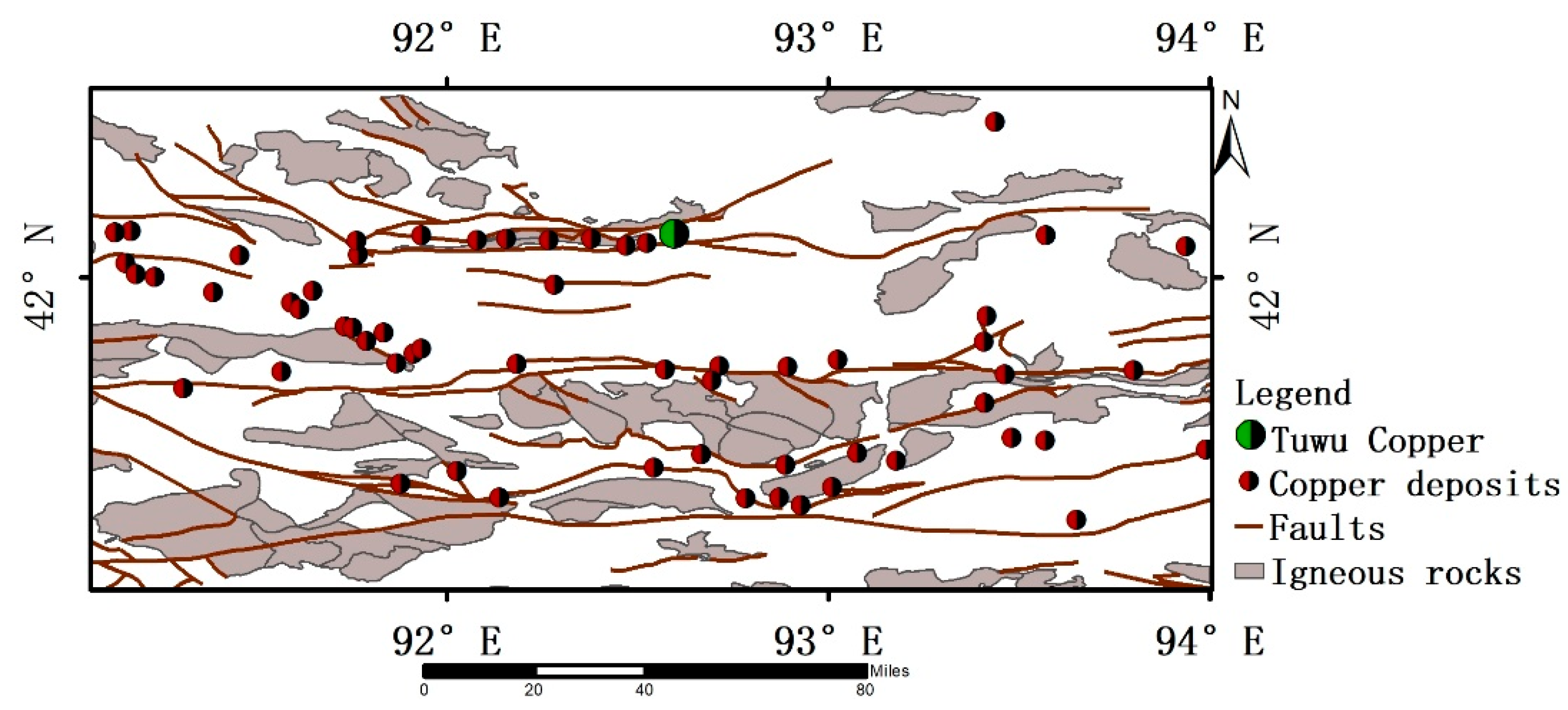
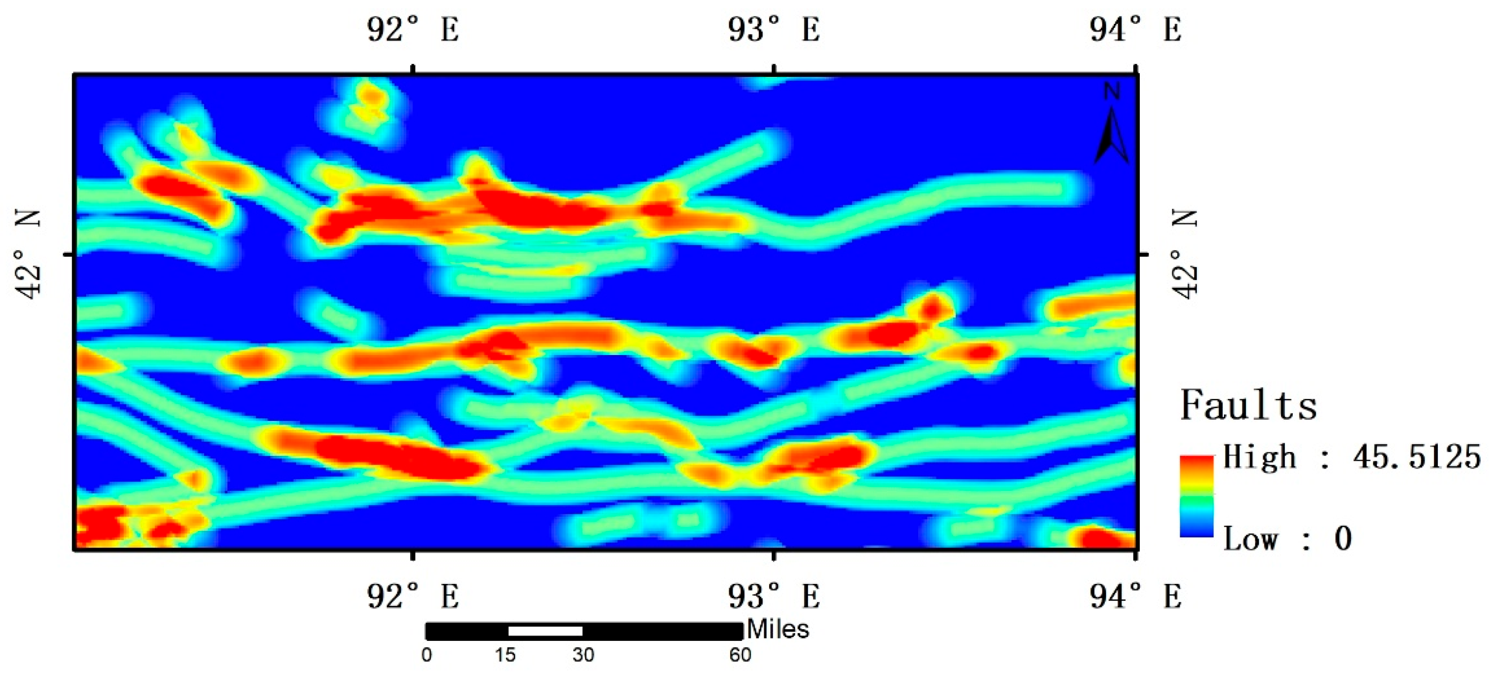
Vector map layers representing magmatic strata and major fault structures were extracted as key evidential layers for mineralization analysis (Figure 4). Additionally, we extract raster layers of igneous rocks (Figure 5) and faults (Figure 6) using the ArcGIS platform to support subsequent spatial modeling and mineralization prediction.

4.2. Remote Sensing Alteration Extraction Results

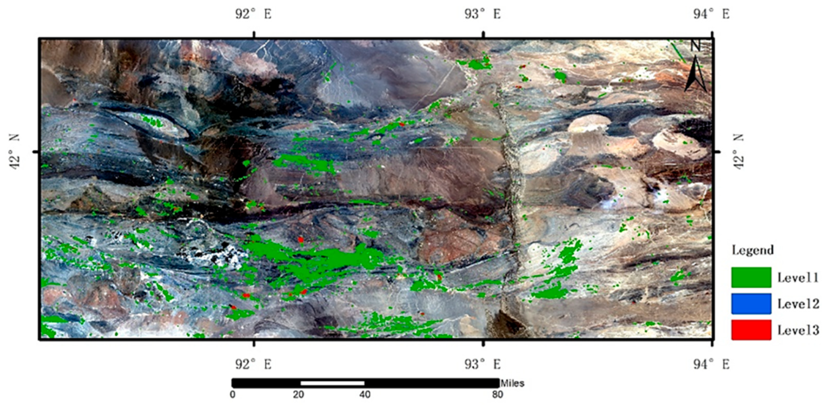
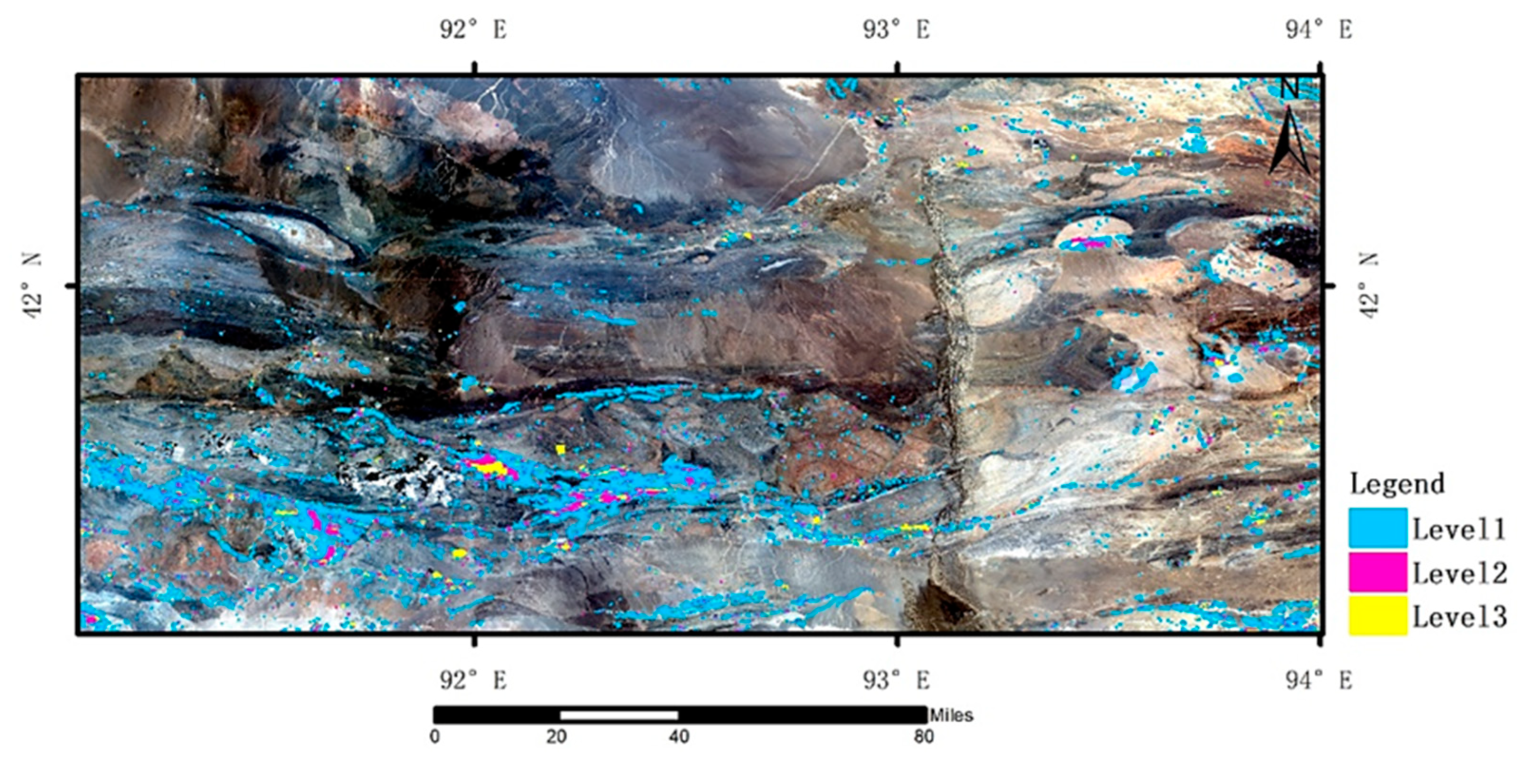
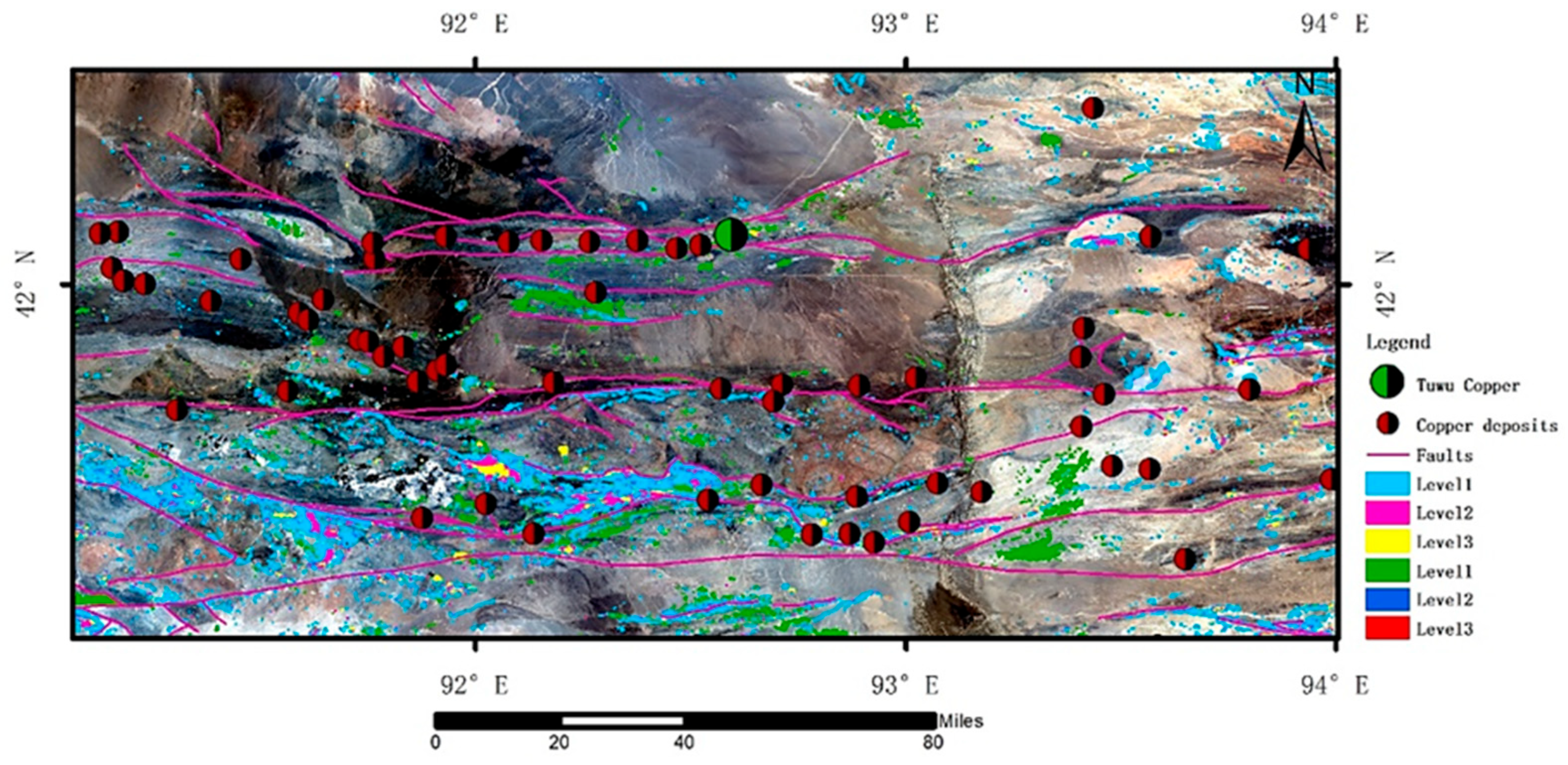
This study utilizes the spectral sensitivity of the Landsat 8 OLI sensor in the near-infrared (NIR) and short-wave infrared (SWIR) bands to extract hydroxyl and iron-stained alteration anomalies through Principal Component Analysis (PCA) (Figure 7, Figure 8 and Figure 9). The classification of anomaly intensity reveals that iron-stained anomalies mainly run along the NNW-SSE direction. Their spatial features closely correspond to the regional structural lineaments. These anomalies display a clear banded pattern along the sides of the Kangguertag-Huangshan fault zone and the Aqikkuduk-Shaquanzi fault zone. Importantly, the areas with concentrated iron-stained anomalies correlate strongly with known copper mineralization points. This suggests that these anomalies can indicate copper enrichment zones.

Hydroxyl alteration anomalies exhibit a similar spatial distribution to the iron-stained zones. Their main bodies also display banded arrangements along major fault structures, with anomaly intensity gradually decreasing from the fault cores toward their margins. This distribution pattern is characteristic of epithermal mineralization systems. The presence of alteration assemblages such as kaolinization and sericitization within these zones provides direct surface evidence of supergene mineralization processes.

Significant overlapping zones of dual (iron-stained and hydroxyl) anomalies occur in the southern segment of the Aqikkuduk Fault and the eastern segment of the Shaquanzi Fault. These overlap zones correspond closely to the regional porphyry–skarn copper metallogenic belt. Considering the Late Paleozoic tectono-magmatic evolution of the eastern Tien Shan, the double-anomaly superposition zone in the northwestern part of the study area aligns spatially with Carboniferous intermediate-acid intrusive bodies. This spatial correspondence reflects the typical metallogenic characteristics of porphyry copper deposits, where alteration centers are structurally controlled. Therefore, the extraction of alteration anomaly information provides valuable metallogenic evidence and supports comprehensive mineral prospectivity analysis in the region.

4.3. Extraction of Geochemical Anomaly Information

According to the regional geological background and research objectives, the target element is Cu. Therefore, based on correlation analysis and relevant literature references [45,46], 14 copper-friendly elements were selected, including Ni, Co, Cr, Mn, P, Ti, V, Zn, Fe, Ag, Au, Mo, Pb, in total. Firstly, outliers were removed from the dataset, and the lower limits of anomalies for each element were determined based on the 85% CFM [47]. The correlation coefficients and lower limits of anomalies between each element and copper are shown in

Table 3. Correlation coefficients and lower limit of anomaly for each element with Cu.

Element	Correlation Coefficient with Cu	The Lower Limit for Anomalies
Ag	0.123	63
Au	0.036	2
Co	0.577	12.375
Cr	0.336	51.9
Cu	1.000	31.08
Mn	0.509	814
Mo	0.176	1.064
Ni	0.304	23.2
P	0.348	631.49
Pb	0.015	19.9
Ti	0.472	3816
V	0.588	94.2
Zn	0.473	66
Fe	0.583	4.86

.

Based on the IBM SPSS Statistics 27.0.1 software platform, factor analysis was conducted on 14 copper mineralization elements. The KMO and Bartlett test results showed that the KMO value was 0.891, greater than 0.6, with a significance level of 0 and less than 0.05, meeting the double test criteria [38]. The corresponding explanatory total variance (

Table 4. The factor explains the total variance of the original variable.

Ingredient	Raw Eigenvalues			Extract the Sum of the Squares of the Loads			Rotating Load Sum of Squares
	Total	Percentage of Variance	Accumulate	Total	Percentage of Variance	Accumulate	Total	Percentage of Variance	Accumulate
1	5.696	40.689	40.689	5.696	40.689	40.689	4.982	35.589	35.589
2	1.552	11.087	51.776	1.552	11.087	51.776	2.014	14.384	49.973
3	1.291	9.219	60.995	1.291	9.219	60.995	1.543	11.022	60.995

) and rotation component matrix (

Table 5. Rotate the composition matrix.

Variable/Element	1	2	3
Ag	0.096	−0.053	0.743
Au	−0.011	0.035	0.172
Co	0.749	0.503	−0.044
Cr	0.277	0.885	0.031
Cu	0.670	0.187	0.165
Mn	0.766	0.105	0.098
Mo	0.120	−0.007	0.546
Ni	0.220	0.896	0.072
P	0.651	0.053	0.032
Pb	−0.067	0.014	0.689
Ti	0.858	0.185	−0.132
V	0.884	0.199	−0.063
Zn	0.694	0.013	0.343
Fe	0.899	0.218	−0.055

) were further obtained. As shown in Table 4, three extracted factors together accounted for 60.995% of the total variance of the 14 original variables, indicating minimal information loss and a satisfactory factor structure. Therefore, these three factors were selected for further interpretation and spatial analysis.

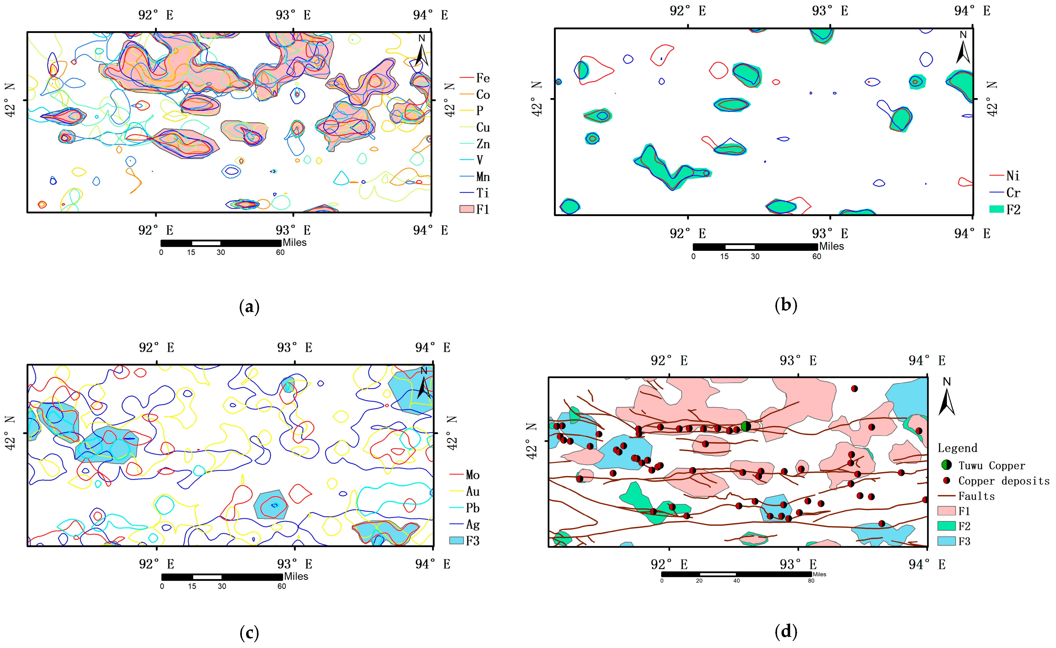
The composition of each factor was determined based on the loadings of individual elements, reflecting their behavior under specific geological processes. The rotated component matrix (Table 5) indicates that three principal factors, each with eigenvalues greater than 1, were extracted: F1 (Co–Cu–Mn–P–Ti–V–Zn–Fe), F2 (Cr–Ni), and F3 (Ag–Au–Mo–Pb). Factor scores were subsequently used to study the spatial distribution characteristics of elements associated with different metallogenic processes.

Based on the spatial overlap relationship between different elements, define all anomalies with overlapping spatial positions as composite anomalies, and plot the anomalies of each element in the same factor on the same graph. Based on the geological background, artificially screen and eliminate abnormal areas with poor mineralization geological conditions and target element combinations within the region. For comprehensive anomalies with relatively large distribution areas, combined with geological conditions and the combination characteristics of elements composed of the same and different factors, artificial segmentation is used to determine the combination anomalies of each element.

Ultimately, this study identified a total of 76 composite anomalies, including 43 F1 (Co–Cu–Mn–P–Ti–V–Zn–Fe) anomaly zones (Figure 10a), 16 F2 (Cr–Ni) anomaly zones (Figure 10b), and 17 F3 (Ag–Au–Mo–Pb) anomaly zones (Figure 10c). According to the delineation of anomalies based on various factors, a comprehensive geochemical anomaly delineation map (Figure 10d) was obtained. Analysis shows that the geochemical delineation anomalies are close to the overall trend of the fault, and are mostly distributed near the fault, with good overlap with known copper deposits and strong prospecting potential.

4.4. Integration of Information on Favorable Elements for Mineralization

Based on the ArcGIS Pro platform, we extracted raster layers of five key metallogenic elements: geological structure, spatial distribution of magmatic rocks, geochemical synthesis anomalies, hydroxyl, and iron-stained advanced alteration. We use bilinear interpolation for spatial standardization to unify the layers to the same spatial resolution and to achieve row-column alignment. Then, we integrate the elemental layers into a 5-channel comprehensive dataset with strictly matched spatial coordinates by using multiband raster synthesis technology. While this multi-channel raster input represents the data-integration stage, the subsequent KDCGAT framework transforms it into a graph-based representation where geological knowledge defines the spatial adjacency and contextual interactions between cells. This step moves beyond data stacking and operationalizes expert knowledge through graph connectivity and adaptive attention weighting. These layers were resampled to match in image size and channel dimensions. Each layer was combined into bands, resulting in a comprehensive raster layer with five band features (Figure 11).

4.5. Model Performance

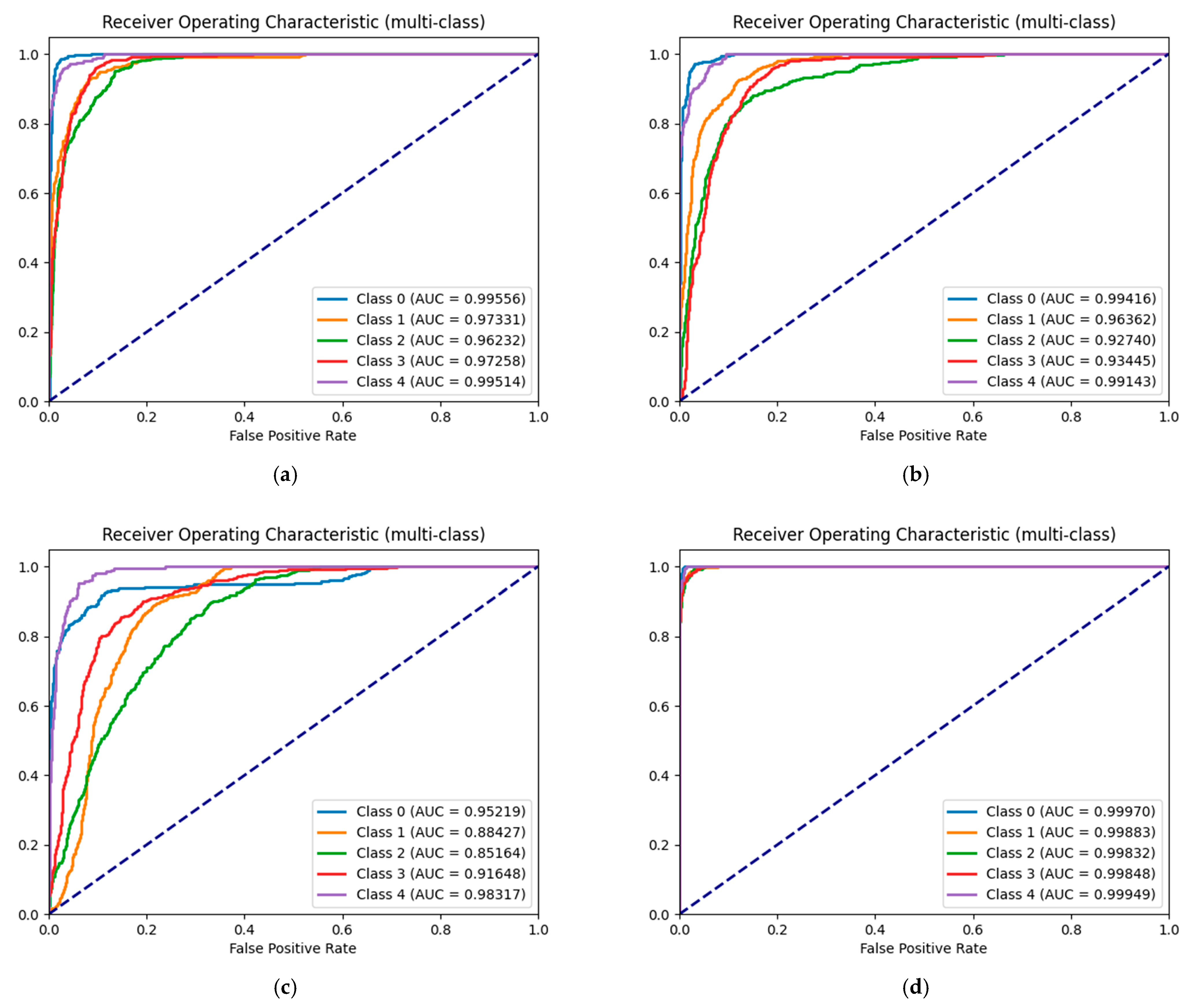
All experiments in this research model were conducted on a workstation (2 × 20-core Intel Gold 6133 CPU, 128 GB memory, and 48 GB VRAM RTX 4090 GPU). Figure 12 presents the ROC curves and AUC values for the four models: (a) WoE, (b) GCN, (c) CNN, and (d) KDCGAT. As shown, the proposed KDCGAT model achieves the highest classification performance across all classes, with AUC values exceeding 0.99 for all categories. The ROC curves of KDCGAT are consistently closer to the upper-left corner, indicating a stronger ability to distinguish between ore-bearing and barren samples.

In contrast, the WoE and CNN models exhibit lower AUC values (mostly between 0.85 and 0.96), suggesting a weaker capability to capture complex nonlinear and spatial dependencies in geological data. Although the GCN model improves upon CNN by introducing graph structural learning, its AUC values (0.93–0.97) are still slightly lower than those of KDCGAT, mainly because GCN treats neighboring nodes with uniform importance.

By incorporating an attention mechanism that adaptively weighs node relationships based on geological knowledge, KDCGAT enhances the representation of both local and regional spatial dependencies. This leads to more robust classification boundaries and improved discrimination accuracy, particularly for the complex and overlapping mineralization zones. Therefore, the ROC and AUC analyses quantitatively confirm that KDCGAT provides the most reliable and discriminative performance among all tested models.

4.6. Model Prediction Results and Comparative Analysis

This study applied the KDCGAT model to predict potential copper mineralization zones within the study area, establishing a knowledge–data dual-driven prediction framework. To evaluate model performance, the predictive capabilities of KDCGAT were compared with three representative models: the traditional Weight-of-Evidence (WOE) method, and two deep learning models—Graph Convolutional Network (GCN) and Convolutional Neural Network (CNN).

Prediction maps for each model are shown in Figure 13. Multi-dimensional validation (

Table 6. Proportion of sites in each model prediction area Each of the four models predicts the proportion of stations in the predicted area.

Models	Level 1	Level 2	Level 3
WOE	24/71 (33.8%)	35/71 (49.3%)	56/71 (78.9%)
GCN	19/71 (26.8%)	31/71 (43.7%)	53/71 (74.6%)
CNN	8/71 (11.3%)	27/71 (38.0%)	47/71 (66.2%)
KDCGAT	27/71 (38.0%)	40/71 (56.3%)	63/71 (85.9%)

) gathered 71 known copper sites, including the Tuwu copper mine. The KDCGAT model’s level 1 prediction area contains 38.0% of these sites. The level 2 area covers 56.3%, and the level 3 area includes 85.9%. This represents a 7%, 11.3%, and 19.7% improvement in accuracy over the WOE, GCN, and CNN models, respectively.

Although the WOE model achieved relatively high accuracy, its reliance on linear statistical assumptions limits its ability to capture nonlinear spatial relationships between evidential layers and ore occurrences. Consequently, it tends to produce fragmented grid-based predictions, insufficiently reflecting the geological controls on mineralization and lacking interpretability [48].

The GCN model, which employs a symmetrically normalized adjacency matrix, exhibited an overall prediction pattern similar to that of KDCGAT. However, due to the over-smoothing effect caused by its fixed aggregation rules, the boundary precision of its predictions was lower. In contrast, the CNN model, implemented based on a U-Net architecture to process rasterized evidential layers, is constrained by Euclidean spatial assumptions. This leads to higher prediction errors when modeling non-Euclidean relationships inherent in geological data.

These comparative experiments clearly demonstrate the advantages of the KDCGAT model. The attention mechanism effectively captures nonlinear interactions among multiple evidential layers, while the knowledge embedding module enhances model interpretability. By integrating geological process understanding with deep learning inference, the KDCGAT model significantly improves the reliability and practicality of mineral prospectivity prediction. The proposed “fracture–rock body–alteration–geochemical anomaly” quaternary attention subnetwork provides a robust decision-support basis for identifying regional copper mineralization targets.

4.7. Ablation Experiment

To test the “knowledge–data” collaboration driven method for predicting copper ore, this paper sets up an ablation experiment. It compares the KDCGAT model with the GAT baseline model, which does not use geological data. The results include a prediction map (Figure 14) and an accuracy table (

Table 7. Proportion of sites in each model prediction area.

Models	Level 1	Level 2	Level 3
GAT	25/71 (35.2%)	28/71 (39.4%)	46/71 (64.8%)
KDCGAT	27/71 (38.0%)	40/71 (56.3%)	63/71 (85.9%)

) for different prediction zones. The experiments show that the GAT model only predicts 25 points in the Level 1 area, 28 points in the Level 2 area, and 46 points in the Level 3 area. KDCGAT improves prediction accuracy by 2.8%, 16.9%, and 21.1% compared to Baseline GAT at each level, while keeping other conditions the same.

The 21.1% improvement achieved by KDCGAT over the baseline GAT is not merely due to the inclusion of additional geological features. Rather, it stems from the integration of domain knowledge into graph construction and attention-based feature propagation. By embedding geological connectivity information—such as faults and lithological boundaries—into the adjacency structure, and allowing attention weights to reflect the relative influence of neighboring geological units, KDCGAT effectively captures knowledge-driven spatial dependencies. This confirms that the proposed model performs genuine knowledge integration rather than simple data aggregation.

These results validate the effectiveness of the knowledge–data dual-drive framework for copper prospectivity prediction. They also highlight the performance gap between traditional purely data-driven models and models informed by geological knowledge, providing a solid theoretical foundation for further research in knowledge-guided mineral prediction.

4.8. Circling and Evaluation of Forecast Areas

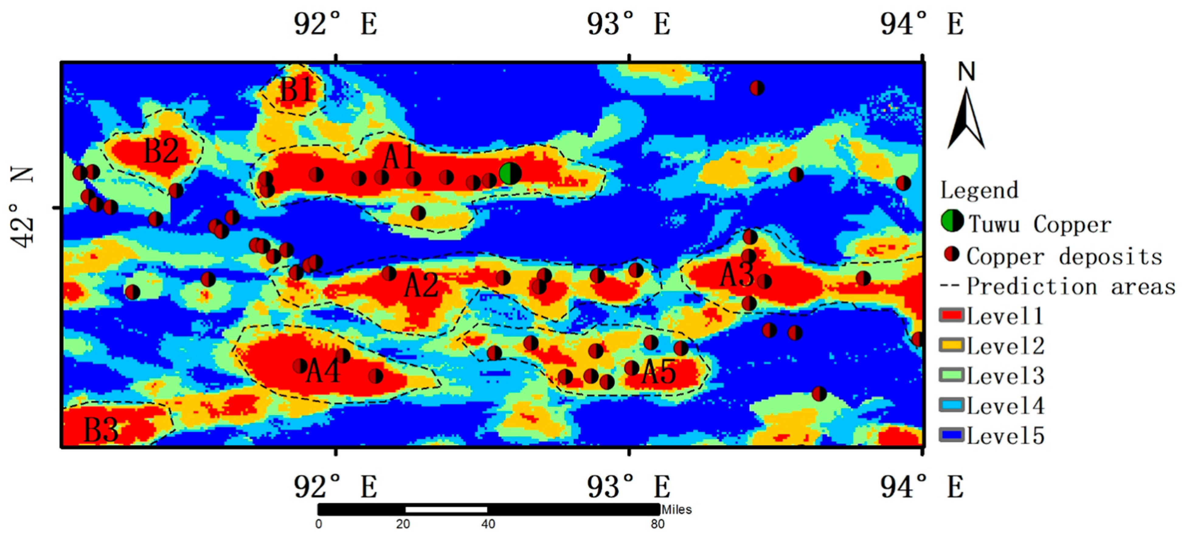
Using the KDCGAT model for prediction and training, this study identifies eight mineralization prediction areas based on mineralization conditions and search indicators. Following the prediction area circling principle, these areas are split into 5 Class A and 3 Class B (Figure 15). Each area is described below:

A1: This zone is located within the Kangurtag–Huangshan Fault Zone, along the southern margin of the Turpan–Hami Basin. It encompasses the well-known Tuwu–Yandong porphyry copper deposits. The dominant fracture orientations are nearly east–west, northwest, and northeast. The exposed strata primarily include the Carboniferous Pengquanshan Group, the Jurassic Xishanyao Formation, and Quaternary deposits. Copper mineralization mainly occurs in the Carboniferous plagioclase granite porphyry and the Pengquanshan Group, defining a Co–Cu–Mn–P–Ti–V–Zn–Fe high anomaly zone.

A2 and A3: These prediction zones cover several known deposits within the Achishan–Yamansu island arc belt. The principal stratigraphic units include the Ordovician Yamansu Formation and the Silurian Achishan Formation. Porphyry copper mineralization is primarily hosted in the Lower Devonian andesitic volcanic and subvolcanic rocks, forming another Co–Cu–Mn–P–Ti–V–Zn–Fe enrichment zone.

A4 and A5: These zones are situated within the Achikkuske–Shaquanzi Fault Zone of the Middle Tien Shan Island Arc Belt, where several known mineralization sites are distributed. The Ordovician–Devonian volcano-sedimentary rock series serves as both the source and the host for mineralization. Devonian–Carboniferous intermediate–acid magmatism provided ore-forming fluids, while the Achikkuske–Shaquanzi Fault and its subsidiary structures acted as conduits for hydrothermal fluid migration and ore precipitation.

B1, B2, and B3: Although no known copper deposits have been identified within these three prediction zones, they exhibit favorable tectonic, stratigraphic, and magmatic conditions for mineralization. The strong spatial coincidence of geochemical and alteration anomalies indicates promising metallogenic potential. These zones are therefore considered prospective copper targets worthy of further geological and geochemical exploration.

5. Conclusions and Discussion

The KDCGAT model for copper mining was constructed based on the fusion of GAT and multimodal geoscience data. It has been applied in the eastern Tien Shan copper mine in Xinjiang. The main conclusions are as follows:

(1)

The accuracy of KDCGAT in copper prediction reaches 85.9%, which is 7%, 11.3%, and 19.7% higher than that of Weight of Evidence (WoE), Graph Convolutional Network (GCN), and Convolutional Neural Network (CNN), respectively. The ablation experiment confirms that the geological knowledge-driven module improves the prediction accuracy of KDCGAT by 21.1% compared with that of the baseline GAT model, which verifies the key role of the “knowledge–data” collaborative framework in reducing the over-smoothing effect and optimizing the allocation of feature weights.

(2)

The data standardization process on the ArcGIS platform combines five key metallogenic elements: fractures, magmatic rocks, hydroxyl/iron-stained erosion, and geochemical anomalies. It creates standardized feature cubes and offers quality inputs for global–local feature aggregation in GAT.

(3)

The model identified eight zones for mineralization prediction. The A1-A5 zones are closely linked to known mine sites. The Class B zones suggest possible exploration targets. This provides a strong basis for future exploration.

While the KDCGAT framework demonstrates strong predictive performance in the eastern Tien Shan, we acknowledge that its effectiveness may vary in geologically distinct regions due to differences in tectonic evolution, lithology, and mineralization patterns. When applied to other metallogenic belts, recalibration or fine-tuning of model parameters and attention weights using local geological, geochemical, and geophysical data may be necessary. Nevertheless, the methodology is inherently generalizable. Its graph-based architecture can flexibly integrate heterogeneous, partially missing, and multi-scale datasets, making it well suited for application to polymetallic and concealed ore systems characterized by data sparsity and complex geological structures. Such adaptability underscores the potential of KDCGAT as a transferable framework for mineral prospectivity mapping across diverse tectonic environments.

In the future, we will further explore the integration of 3D geological modeling with dynamic processes. Currently, temporal evolution information of tectonic deformation and hydrothermal fluid migration is unavailable at sufficient spatial resolution, which limits the model to static predictions. Extending the current 2D framework to 3D geological modeling will allow the incorporation of stratigraphic depth, fault dip, and subsurface alteration zones, enabling more accurate characterization of complex ore-forming systems in both space and time.