Mineral Prospectivity Mapping for Exploration Targeting of Porphyry Cu-Polymetallic Deposits Based on Machine Learning Algorithms, Remote Sensing and Multi-Source Geo-Information

Abstract

Machine learning (ML) algorithms have promoted the development of predictive modeling of mineral prospectivity, enabling data-driven decision-making processes by integrating multi-source geological information, leading to efficient and accurate prediction of mineral exploration targets. However, it is challenging to conduct ML-based mineral prospectivity mapping (MPM) in under-explored areas where scarce data are available. In this study, the Narigongma district of the Qiangtang block in the Himalayan–Tibetan orogen was chosen as a case study. Five typical alterations related to porphyry mineralization in the study area, namely pyritization, sericitization, silicification, chloritization and propylitization, were extracted by remote sensing interpretation to enrich the data source for MPM. The extracted alteration evidences, combined with geological, geophysical and geochemical multi-source information, were employed to train the ML models. Four machine learning models, including artificial neural network (ANN), random forest (RF), support vector machine and logistic regression, were employed to map the Cu-polymetallic prospectivity in the study area. The predictive performances of the models were evaluated through confusion matrix-based indices and success-rate curves. The results show that the classification accuracy of the four models all exceed 85%, among which the ANN model achieves the highest accuracy of 96.43% and a leading Kappa value of 92.86%. In terms of predictive efficiency, the RF model outperforms the other models, which captures 75% of the mineralization sites within only 3.5% of the predicted area. A total of eight exploration targets were delineated upon a comprehensive assessment of all ML models, and these targets were further ranked based on the verification of high-resolution geochemical anomalies and evaluation of the transportation condition. The interpretability analyses emphasize the key roles of spatial proxies of porphyry intrusions and geochemical exploration in model prediction as well as significant influences everted by pyritization and chloritization, which accords well with the established knowledge about porphyry mineral systems in the study area. The findings of this study provide a robust ML-based framework for the exploration targeting in greenfield areas with good outcrops but low exploration extent, where fusion of a remote sensing technique and multi-source geo-information serve as an effective exploration strategy.

1. Introduction

Mineral prospectivity mapping (MPM) is considered an advanced and effective method in mineral exploration, which aims to search for mineral prospectivity of specific types in unexplored areas and to delineate high-potential regions of the sought mineralization. MPM is essentially a binary classification issue from the algorithmic perspective [1], that is, to judge whether mineral deposits are present or absent in each unit based on the predicted probability. Its modeling process can be understood as relating a series of evidential features (input variables) to the presence of the target deposit (output variables) by establishing a synthetic function [2]. Generally, MPM can be categorized into two primary types, namely knowledge-driven and data-driven, based on their different manners in combining evidential data and estimating model parameters by expert judgement (knowledge-driven) or by using objective ore-related data (data-driven). The former, such as fuzzy logic and the fuzzy analytic hierarchy process [3,4], is suitable for areas where there are no or few mineral deposits (greenfield areas); while the latter, such as classical weights-of-evidence and evidence belief [5], is applicable for areas with sufficient mineral deposits and rich ore-forming data information (brownfield areas). Among them, data-driven MPM is more widely accepted because it is objectively supported by the correlation between geological features and mineral deposits rather than subjectively employing expert knowledge to heuristically estimate model parameters [6]. However, although the traditional data-driven methods can objectively reflect the relationship between geological features and deposits, they are unable to address high-dimensional and nonlinear geo-information. Compared with the traditional data-driven MPM methods, machine learning (ML)-based MPM, which is implemented via ML methods, has significant advantages in processing complex and nonlinear multi-source geological data [7,8]. It constructs effective prospectivity models to classify the target regions into favorable and unfavorable zones [9]. In recent years, with the rapid development of ML algorithms, there have been many ML methods successfully applied to MPM, some commonly used ML models include artificial neural network (ANN) [10,11,12], support vector machine (SVM) [13,14], random forest (RF) [15,16], convolutional neural network [17,18], etc. It is important to note, however, that although ML methods have been proven to perform well in MPM, no single model has been verified to perform best in all situations [2]. Therefore, modeling with multiple ML models and comparative studies of the models are indispensable in MPM studies [19].

In many MPM instances, the occurrence locations in a specific area, which are products of rare mineralization events, are often extremely scarce, while non-occurrence locations are relatively widely distributed and easy to select [20,21,22], which results in a highly imbalanced training dataset, that is, the number of negative samples far exceeds that of positive samples. However, in ML applications, when dealing with training datasets with unbalanced positive and negative samples, the supervised learning model often fails to train the dataset well, and the predictions would be more biased to majority classes and ignore minority classes [23,24]. To address this shortcoming, many studies have employed the synthetic minority over-sampling technique (SMOTE) to generate synthetic data for the minority classes to balance the dataset [25,26], and the results demonstrated that such application can improve the performance of ML models [27,28].

Remote sensing is effective in extracting lithologic units, alteration types, structures and indicator minerals of specific ore deposits [29]. Compared with traditional explorative tools, remote sensing is deemed the most economical data source in large research areas with difficult terrain and exploration extent [30]. In ML-based MPM, a variety of remote sensing imaging techniques have been utilized to obtain source data of evidence layers, such as hyperspectral imaging, multispectral imaging and radar imaging [31]. Among them, multispectral imaging is widely used for the extraction of alteration information due to its advantages of simplified bands, moderate resolution, less data redundancy and fast processing speed [32]. Many scholars employ remote sensing enhancement techniques, including the band ratio method, principal component analysis (PCA), independent component analysis and minimum noise fraction to extract specific band information from high-dimensional multi-spectral remote sensing images, and highlight the spectral reflectance characteristics of the band combination in the new low-dimensional space [29,33]. According to the reflectance characteristics, the distribution of one or a class of ore-related alteration in a regional scale can be extracted [34,35,36]. Such information was used together with multi-source geological feature data to generate evidence layers for MPM.

The Narigongma area, recognized for its significant metallogenic potential following the discovery of the Narigongma porphyry deposit, was selected as the study area. The area is characterized by a high altitude, challenging terrain and inconvenient transportation, making it extremely challenging for traditional explorative methods [37]. However, due to the sparse coverage of surface vegetation, this area is highly conducive to the application of remote sensing techniques. The purpose of this study is to predict the ore-forming potential of porphyry Cu-polymetallic deposits in the study area through the analysis of interpreted remote sensing images and by integrating multi-source evidential feature information to train ANN, RF, SVM and logistic regression (LR) models. The predictive performances of the models were evaluated by confusion matrices and success-rate curves. The targets of Cu-polymetallic mineralization identified by the optimal predictive model provide instrumental insights for future mineral exploration.

2. Geology of the Study Area

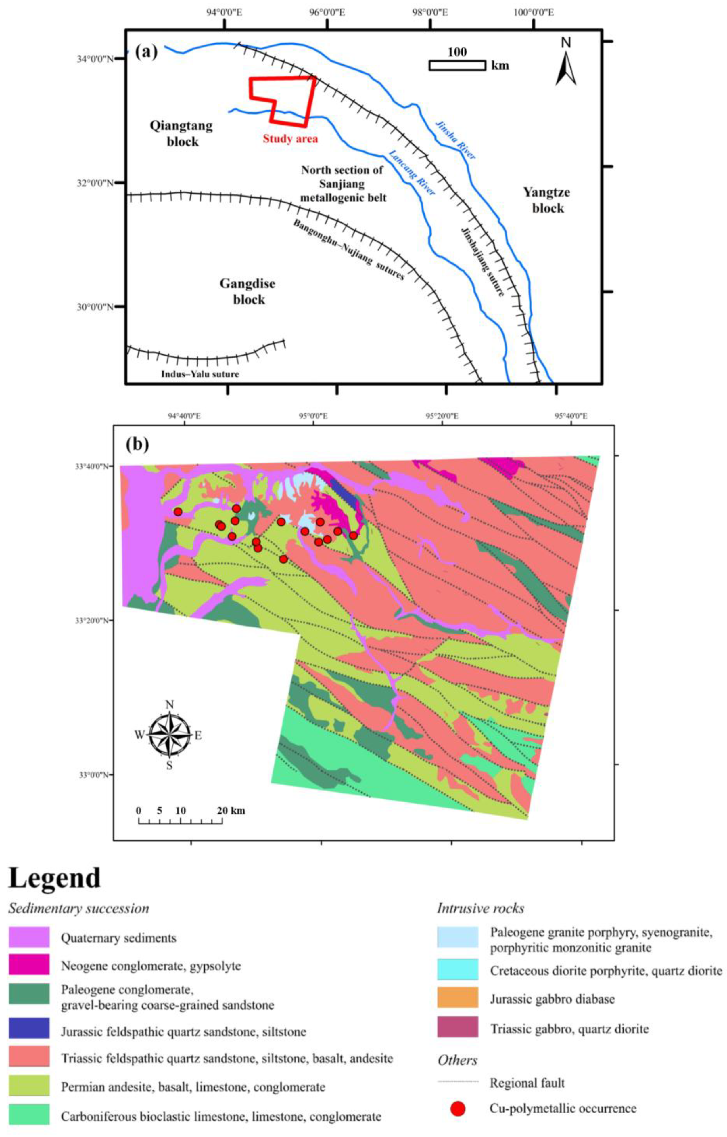
Narigongma area is situated in the Qiangtang block of Himalayan–Tibetan orogen, pertaining to the north section of the famous Sanjiang metallogenic belt in western China (Figure 1a). The Qiangtang block is bounded by the Bangonghu-Nujiang sutures to the south and the Jinshajiang suture in the north (Figure 1a). The Qiangtang block holds a set of porphyry Cu deposits, including the renowned Yulong deposit and Narigongma deposit, which are found to be formed in a post-collisional setting [38]. The Neo-Tethyan Ocean was subducted northwest beneath the Lhasa block from the Early Jurassic to Late Cretaceous [39]. The closure of Neo-Tethyan Ocean and collision of India and Asia were believed to occur at 70–60 Ma [37,39], leading to the formation of the Himalayan orogen. After the India–Asian collision, the Qiangtang block in the Himalayan orogenic belt transitioned into a post-collision regime, which gave rise to a series of tectonic–magmatic events that is responsible for the Cu-polymetallic mineralization in this region [37,40].

The intrusive rocks outcropped in the study area are mainly granitic rocks (Figure 1a), dominated by biotite granite porphyry and fine-grained granite porphyry. The biotite granite porphyry surrounding the ore bodies yielded a zircon U-Pb age of 41.53 ± 0.24 Ma [41,42], which is close to the mineralization age indicated by the molybdenite Re-OS age of 40.86±0.85 Ma of mineralized veins in the Narigongma deposit [40]. The porphyry intrusions were emplaced into Permian and Triassic volcanic–sedimentary sequences, which consist of basalt and andesite interbedded with sandstone, siltstone and muddy limestone (Figure 1b). The emplacement of the porphyry resulted in the contact metamorphism of sedimentary wall rocks, forming a characteristic metamorphic zone consisting of outer marbles, intermediate skarns and inner hornfels [37]. The NW-trending faults constructed the main structural framework in this area, which accords with the direction of the regional tectonic lines (Figure 1a) and controls the distribution of sedimentary successes and emplacement of intrusions (Figure 1b).

Figure 1. Maps of the study area: (a) the tectonic location of the study area, modified from [43]; (b) a simplified geological map of the study area, modified from [44].

Figure 1. Maps of the study area: (a) the tectonic location of the study area, modified from [43]; (b) a simplified geological map of the study area, modified from [44].

The Narigongma deposit contains 0.46 Mt Cu, with an average grade of 0.32 wt.%, and 0.25 Mt Mo, with an average grade of 0.06 wt.% [37,40,45,46]. The Cu-bearing mineral is mainly chalcopyrite, with minor bornite and aikinite, and the Mo-bearing mineral is molybdenite [37]. The deposit exhibits a typical porphyry mineralization–alteration pattern. The Cu-Mo ore bodies primarily occur within the inner and outer contact zones between the porphyry intrusions and wall rocks (Figure 2). Hydrothermal alteration is generally characterized by concentric zones that range from inner potassic alteration through beresitization zones to outer propylitic zones (Figure 2). Potassic alteration was developed within the biotite granite porphyry, manifested as K-feldspar alteration and biotitization. The ore mineral assemblage in the potassic zones consists of pyrite, chalcopyrite and molybdenite. Beresitization alteration was primarily distributed around the potassic alteration zone, characterized by the enlargement of quartz phenocrysts, the appearance of quartz porphyroblasts, local occurrence of quartz veinlets and sericitization along structural fractures. The mineral assemblage comprises quartz + sericite + K-feldspar and ore minerals of pyrite + chalcopyrite + molybdenite. Propylitic alteration was mainly developed in the outer contact zones of porphyry intrusions and their surrounding basalts, where chlorite and epidote replace pyroxene and plagioclase. Compared to the classic alteration zoning pattern of porphyry Cu deposit, the argillic alteration in the Narigongma deposit is not well-developed [47]. The chalcopyrite and molybdenite are disseminated along micro-cracks in quartz veinlets. Most of these veinlets were found to be associated with beresitization alteration [37].

3. Materials and Methods

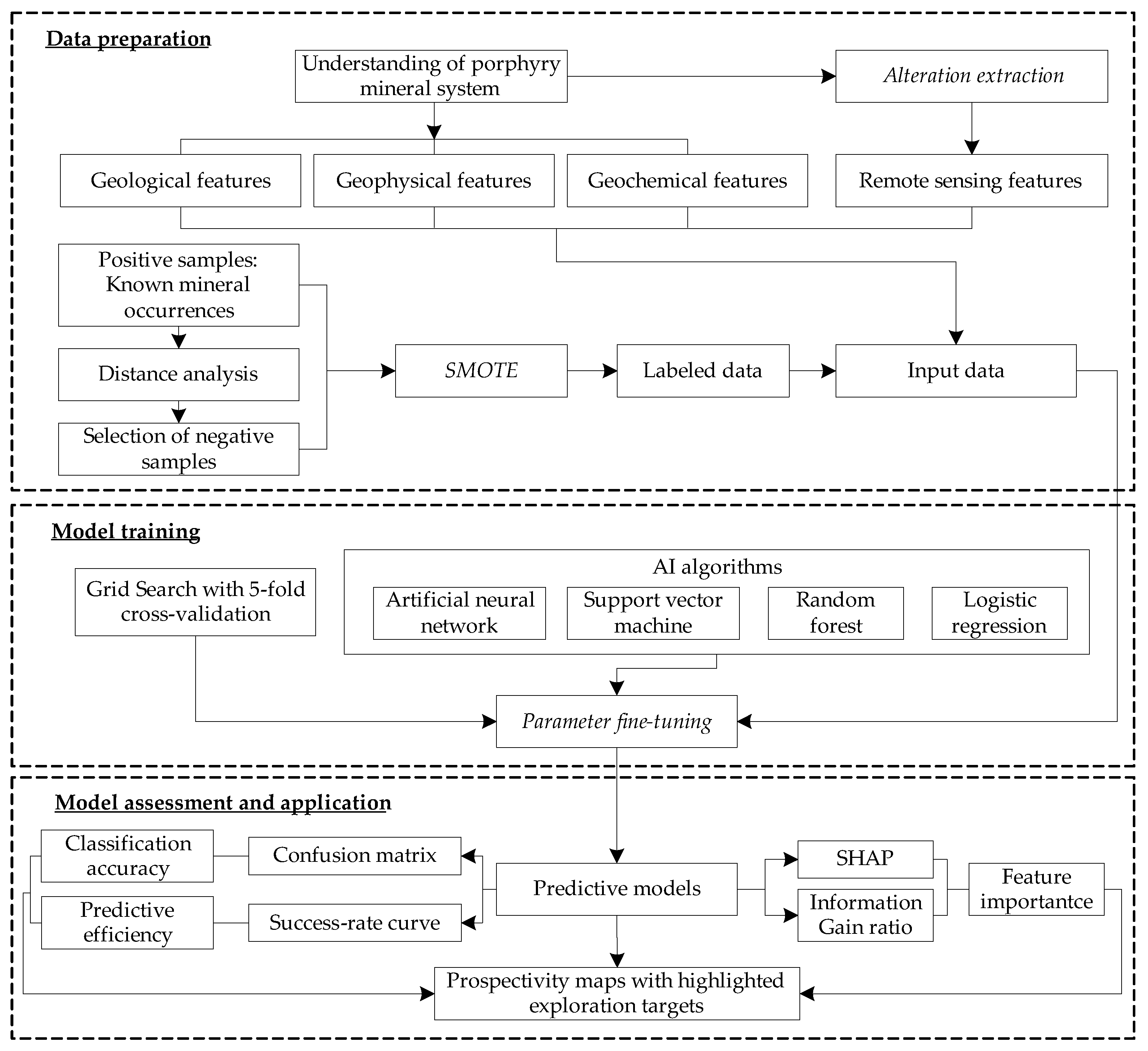
In this study, the MPM was conducted with the aid of a systematic ML-based framework, as presented in Figure 3. The flowchart can be subdivided into data preparation, model training and model assessment and application. Multi-source geo-information related to porphyry mineralization, including geological, geophysical and geochemical information, was collected. The hydrothermal alteration was extracted from remote sensing data. SMOTE was employed to augment scarce training samples. All these works of data preparation were guided by the understanding of porphyry mineral system in the study area. The integrated input data were then fed into the ML algorithms, including ANN, SVM, RF and LR. The grid search with 5-fold cross-validation served as training strategy, allowing for generation of the predictive models configured with the optimal parameters. The resulting models were comprehensively assessed by confusion matrix-derived indices, success-rate curve and interpretability tools, based on which the prospectivity map and exploration targets can be delineated based on the consideration of the classification accuracy, predictive efficiency and feature importance.

3.1. Data Used

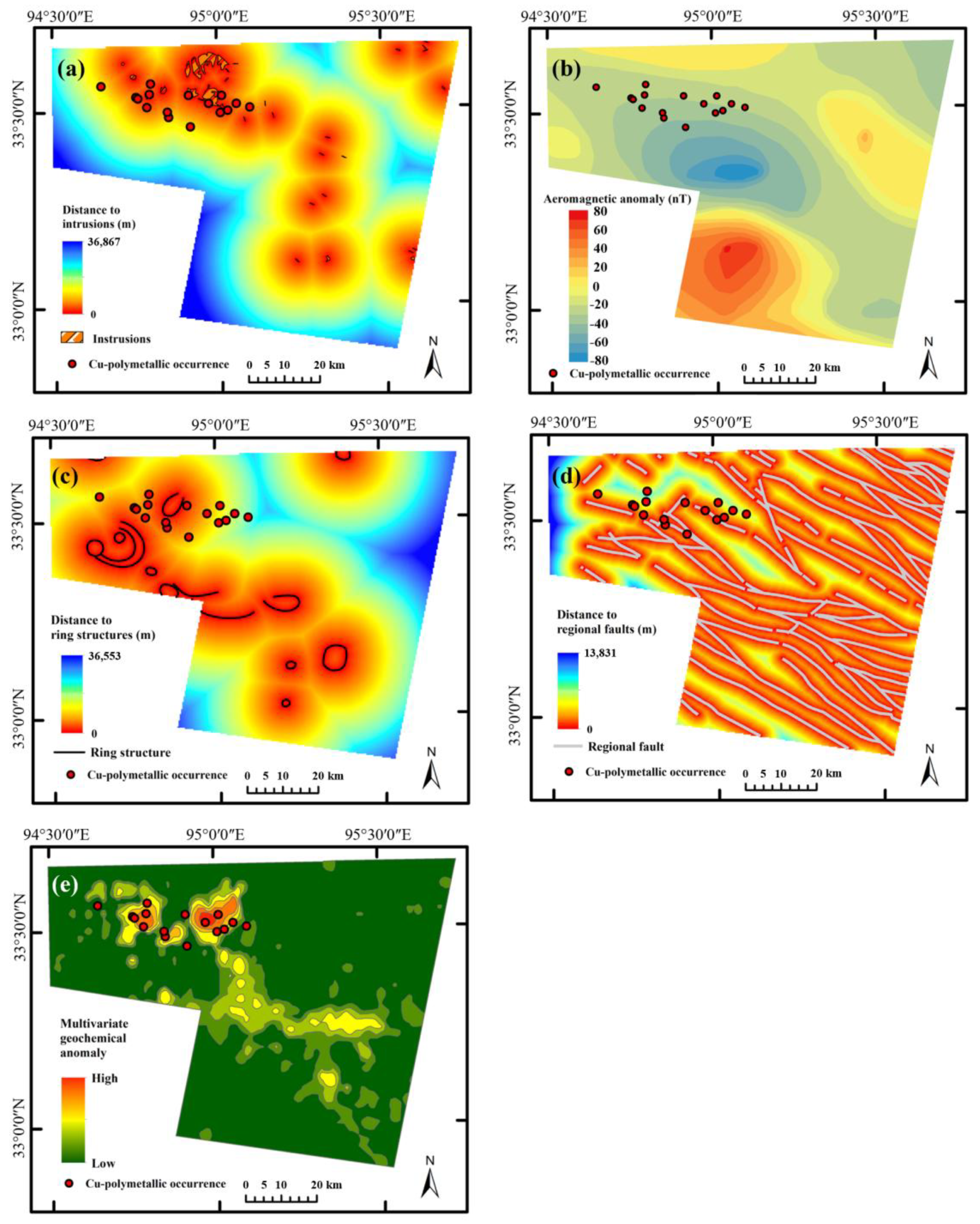
Multi-source geological features related to mineralization, including geological, geophysical, geochemical and remote sensing, were employed in this study. These features were selected according to the understanding of target mineral system. It is widely accepted in previous studies, as presented in Section 2, that the granite porphyry intrusions in the study area are spatially, temporally and genetically associated with the Cu-polymetallic mineralization, and the intrusions are considered to have acted as the source of material and heat that trigger the ore-forming system [37]. Therefore, the proximity to outcropped intrusive rocks was employed as an evidential feature (Figure 4a). In addition, magnetic anomalies (Figure 4b) were collected from a 1:200,000 aeromagnetic survey and utilized to map the concealed intrusive rocks [47], given that there exists an apparent distinction between the intrusions and their surrounding sedimentary rocks. In general, the porphyry deposits are controlled by regional lineaments and ring structures [48], which serve as effective pathways for channeling the ore-related magma from deep seat to upper crust. These features were extracted by remote sensing, and their proximity was considered favorable evidence for mineralization (Figure 4c). The fault networks of caprocks provides important channels for the flow and focusing of metalliferous fluids; therefore, proximity to caprocks faults was employed as an evidential layer (Figure 4d). The ore-related geochemical anomalies are the direct indicators for tracing the target mineralization. In this study, Cu-Mo-W-Co-Ni-Fe-Mn multivariate geochemical anomalies (Figure 4e), representing element combination related to porphyry Cu-Mo mineralization in the study area, were collected and modified from Dong [49]. The multivariate geochemical anomalies were extracted based on the factor analysis, which was conducted on geochemical data of 24 elements derived from 1:200,000 regional geochemical mapping project. The geological features, including intrusions and structural information, were derived from a 1:250,000 Zhidoi County geological map of Qinghai Province, China [44].

The Advanced Spaceborne Thermal Emission and Reflection Radiometer (ASTER) sensor is a multi-spectral imager that was launched on the Terra satellite, which has been in operation since 1999 [50,51]. ASTER scenes can be downloaded from the United States National Aeronautics and Space Administration (https://earthdata.nasa.gov; accessed on 23 September 2025).

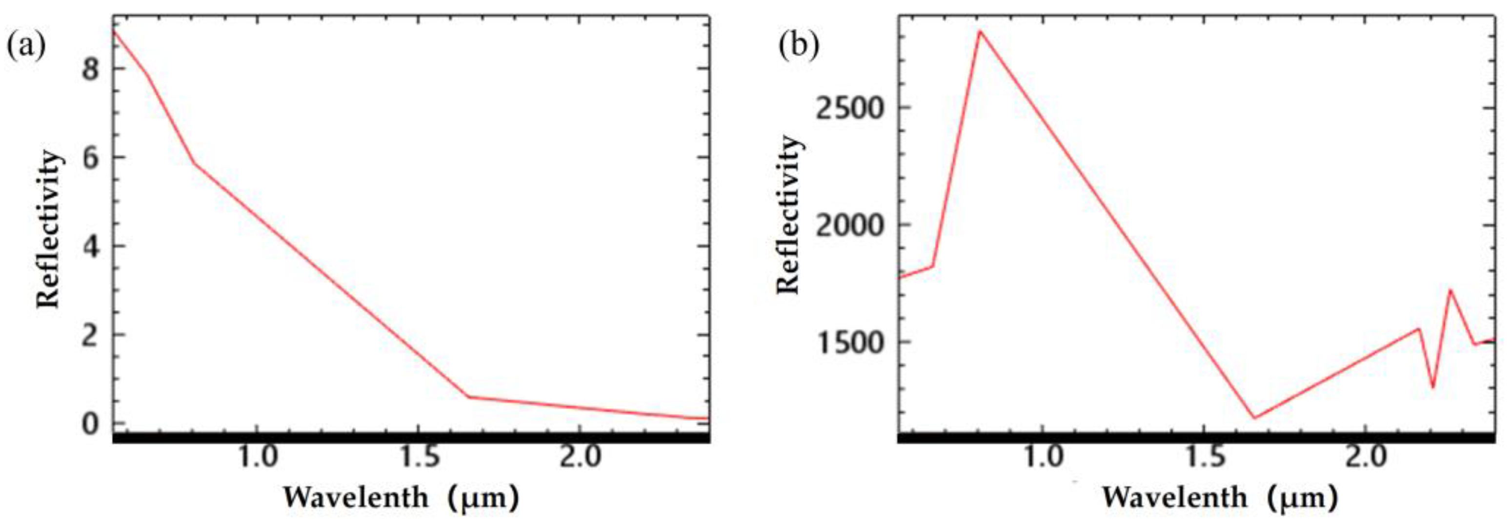
In this study, three L1T ASTER scenes of Zadoi and Zhidoi County in the Qinghai Province were selected to cover the study area. The scenes included one from 28 January 2003 (Granule ID: AST_L1T_00301282003043416_20150427000827_27390) and two scenes from October 9, 2005 (Granule IDs: AST_L1T_00310092005042603_20150511120221_31821 and AST_L1T_00310092005042612_20150511120216_100437). These scenes of imagery from different years have temporal consistency in the task of alteration extraction since hydrothermal alteration is a geological process involving chemical reactions between ore-forming hydrothermal fluids and country rocks, typically spanning geological time scales of thousands to millions of years. Within a brief two-year interval (2003–2005), the physico-chemical properties of altered minerals, including composition, structure and spatial distribution, exhibit no significant changes; therefore, their spectral characteristics in remote sensing imagery remain stable. Furthermore, the ASTER data encompasses 14 spectral bands covering the visible–near infrared (VNIR), short-wave infrared (SWIR) and thermal infrared (TIR) regions. Its VNIR and SWIR bands are particularly sensitive to diagnostic features of alteration minerals. Although temporal differences exist between 2003 and 2005 datasets, the mineral assemblages and their spectral response patterns in a given region do not fundamentally shift due to short-term environmental fluctuations or minor sensor noise. Through pre-processing steps, systematic errors between the two years’ data can be further minimized, ensuring comparability of alteration information. These scenes were clear with minimal vegetation, featuring only slight snow and cloud cover in certain areas, making them suitable for the extraction of mineral alteration information. The low vegetation coverage was emphasized in this study because the alteration minerals primarily occur in ore bodies and country rocks at or near the surface, and their remote sensing signals depend on electromagnetic waves directly reflected or emitted by surface materials. When vegetation is dense, leaves, branches and other plant structures physically obscure the underlying altered rocks. In such cases, remote sensing sensors predominantly capture signals from the top layer of vegetation rather than the alteration minerals, causing alteration information to be physically masked or even completely lost. Given that the alteration information to be extracted has distinct spectral features in the VNIR and SWIR band ranges, it is essential to pre-process these bands. The pre-processing mainly involves radiometric calibration, atmospheric correction, constructing mask to eliminate interference and image mosaicking. All operations were performed using ENVI 5.3, where the FLAASH module was utilized for atmospheric correction, which re-scales raw radiance data (Figure 5a) to reflectance data (Figure 5b) that can be directly compared with the laboratory reflectance spectra. The seamless mosaic module for image mosaicking.

3.2. Alteration Extraction

Remote sensing technology was employed to obtain the information of altered minerals in the study area. PCA is a widely used technique for dimensionality reduction in remote sensing image processing. It involves mapping the information from several key bands, which needs to be highlighted in the high-dimensional and multi-band composite image, onto lower-dimensional spaces through projection. This process eliminates the interference caused by the overlap of irrelevant noise band information, thereby preserving the original information of data in the newly created low-dimensional spaces. In this study, the Crosta method, which is based on PCA, was utilized to highlight the band information of features with fewer dimensions [52], which helped to distinguish abnormal regions and extracted pixel values based on their high and low reflectance levels.

3.3. Synthetic Minority Over-Sampling Technique (SMOTE)

SMOTE is a method employed to solve the over-sampling problem [53]. The principle of SMOTE involves identifying a given sample X_i in the internal feature space of minority class, searching for its N nearest neighbors to the sample and then calculating the difference between the sample and each of these neighbors. To balance the dataset, the method randomly selects a number of these N neighbors based on the required number of synthetic samples and calculates the respective differences. In this study, the default N value of 5 was employed to specify the quantity of nearest neighbors (from X₁ to X₅). For generating one synthetic sample, the difference between X_i and a randomly selected neighbor (X₃ in this case) was calculated. Subsequently, the calculated differential value was multiplied by a random number between 0 and 1, and the resulting value was then added to the sample (Figure 6). The formula for describing above process can be expressed as follows [54]:

$$X_n=X_i+rand\left(\mathrm{0,1}\right)\times (X_3-X_i)$$

(1)

3.4. Machine Learning Methods

3.4.1. Artificial Neural Network (ANN)

ANN is a ML method that imitates the structure and information processing mode of human brain [55]. It is a computational model composed of large number of interconnected nodes, known as neurons, organized into an input layer, one or more hidden layers and an output layer, respectively. Each connection of interconnected neurons is associated with a weight. These weights are adjusted via backpropagation during training [56]. The back propagation neural network is a type of multi-layer feedforward neural network, where the information processing in this network includes two main stages, namely forward propagation of information and back propagation of error. During forward propagation, information flows unidirectionally from the input layer through the hidden layers and then to the output layer according to the connections between different neurons and the weight values assigned to each unit. This process can be expressed by the following formula [57]:

$$y_j=f\left(\sum _i{w}_{tp}{x}_p+b_t\right)$$

(2)

where $w_{tp}$ denotes the weight value connecting the previous layer of neurons $t$ and $p$, $b_t$ represents the deviation of neuron $t$ and $f$ signifies the activation function. The sigmoid activation function employed in this study can be expressed by the following formula [58]:

$$f\left(x\right)={\displaystyle \frac{1}{1+Exp(-x)}}$$

(3)

where $x$ represents the input feature data. The output data is transmitted through the network, followed by the calculation of the error between the output data and the expectation, which is then backpropagated through the network. Backpropagation algorithm is a supervised learning method that consists of two primary stages, namely propagation and weight adjustment. These two steps are repeated continuously until the model training achieves the desired level of accuracy or until the number of training iterations reaches a predetermined limit. Following the conclusion of the training process, the model whose output data most closely aligns with the actual expectations is selected as the final result.

3.4.2. Random Forest (RF)

RF is an ensemble ML approach proposed by Breiman [59]. RF consists of a certain number of complete and independent decision trees. These trees are generated through a process of random sampling known as bootstrap aggregating, where the input data for each tree is randomly selected from the original dataset with replacement. Each sample also randomly selects certain features as the training data for the decision tree by means of putting back. Each node of the tree corresponds to a specific splitting rule, which is applied from the root node to the leaf nodes in turn. The tree iteratively splits the root node into the leaf node until a stopping condition is satisfied, signifying the completion of the training phase. This approach maximizes the purity of the branches resulting from the leaf node splits, and this purity is measured using the Gini index, as described in the formulation provided by Gordon et al. [60]:

$$I_G(f)={\sum }_{i=1}^m{f}_i(1-f_i)$$

(4)

$$f_i={\displaystyle \frac{n_j}{n}}$$

(5)

where $f_i$ denotes the probability of class $i$ at node $m$, $n_j$ represents the number of samples belonging to class $j$ and $n$ signifies the total number of samples of a specific node. The result is determined by the voting of all decision trees in the forest.

3.4.3. Support Vector Machine (SVM)

SVM, proposed by Vapnik [61], is a supervised learning method that distinguishes two different types of samples by constructing a classification boundary. In a two-dimensional space, the SVM model can construct an optimal linear classifier that separate different classes with the widest decision boundaries. In the high-dimensional space, an infinite number of hyperplanes can be obtained, each capable of dividing sample points with various characteristics. The optimal hyperplane is identified as the one that achieves the highest level of separation confidence across the entire dataset. In this study, support vector machine was used for binary classification problems in multi-feature dimensions, specifically distinguishing between occurrence and non-occurrence units. The algorithm assumes a training dataset ${\left\{x_i\right\}}_{i=1}^n$ comprising $n$ feature vectors, each vector is associated with a corresponding label $y_i$. In this study, a $y_i$ value of +1 represented the occurrence unit, and a $y_i$ value of −1 indicated the non-occurrence unit. The input data was initially mapped to a high-dimensional space $P$ by mapping function $\Psi$. In this feature space $P$, the training set was linearly separable, allowing for a hyperplane $S$ that separated the labeled data into two classes. This binary classification can be generated by a set of formulae [1,62]:

$$\left\{\begin{array}{c}w\Psi \left(x_i\right)+b\ge 1-{\sigma }_i , { y}_i=+1\\ w\Psi \left(x_i\right)+b\le -1+{\sigma }_i , y_i=-1\\ {\sigma }_i\ge 0 , i=\mathrm{1,2},\dots ,n\end{array}\right.$$

(6)

Here, $w$ represents the weight vector of the hyperplane, $b$ is the deviation and ${\sigma }_i$ signifies the slack variable. There can be an infinite number of such hyperplanes ($S_0,{ S}_1, S_2$ and $S_n$), but only one hyperplane $S_0$ satisfies the maximum margin requirement. This particular hyperplane is recognized as the optimal hyperplane. According to the optimization function theory, the two parameters $w$ and $b$ for solving the optimal hyperplane can be converted into an optimization problem [63]:

$$\left\{\begin{array}{c}Minimize:{\displaystyle \frac{1}{2}}{\left|\right|w\left|\right|}^2\\ subject to:y_i(w\Psi \left(x_i\right)+b)\ge 1,i=\mathrm{1,2},\dots ,n\end{array}\right.$$

(7)

where this optimization problem can be solved by solving the saddle point of the Lagrange function [63,64]:

$$L(w,z,h)={\displaystyle \frac{1}{2}}{\left|\right|w\left|\right|}^2\sum _{i=1}^n{z}_i{y}_i(w\Psi \left(x_i\right)+h)+\sum _{i=1}^n{z}_i$$

(8)

where $z_i$ (i = 1, 2, …, n) is the Lagrange multiplier obtained by the following optimization function [1,63]:

$$\left\{\begin{array}{c}Maximize:{\displaystyle \sum _{i=1}^n}{z}_i-{\displaystyle \frac{1}{2}}{\displaystyle \sum _{i=1}^n}{\displaystyle \sum _{j=1}^n}{z}_i{z_{j}y}_i{y}_j\Psi \left(x_i\right)\Psi \left(x_j\right)\\ Subjected to:{\displaystyle \sum _{i=1}^n}{z}_i{y}_i=0, 0\le z_i\le C, i=\mathrm{1,2},\dots ,n\end{array}\right.$$

(9)

Here, $C$ is the penalty factor for misclassification error. A kernel function $R$ can be defined as follows:

$$R(x_i,x_j)\Psi \left(x_i\right)\times \Psi \left(x_j\right)$$

(10)

Several commonly used kernel functions include radial basis, linear, polynomial and sigmoid. In this study, the radial basis function was employed due to its low error rates and the simplicity of parameters in the practical applications [1], which can be expressed as follows:

$$R(x_i,x_j)=\mathit{exp}(-\gamma {\left|\right|x_i-x_j\left|\right|}^2), \gamma >0$$

(11)

3.4.4. Logistic Regression (LR)

LR is a multivariate statistical method based on the hypothesis of nonlinear relationship between the occurrence of mineral deposits and geological features [3]. LR describes the relationship between a response variable and one or more explanatory variables, where the response variable is binary, meaning it represents the presence or absence of an occurrence [65]. When the feature dimension of the samples used in training is high, LR can effectively accommodate the conditional dependence in the input data, avoiding the problem of correlation between variables and thus producing less output bias. LR is a simple and efficient method for binary and linear classification problems [66]. Its linear equation can be expressed as follows:

$$\Phi =b_0+b_1{x}_1+b_2{x}_2+b_3{x}_3+\dots +b_n{x}_n$$

(12)

where the $\Phi$ value of 1 represents occurrence, the $\Phi$ value of 0 denotes non-occurrence, $b_0$ is the intercept term of the model, $x_i$ (i = 1, 2, …, n) signifies the independent variable and $b_1-b_n$ is the regression coefficient of the independent variable. Following the logit transformation of the binary response variable through a logical connection function, the regression coefficient of LR is estimated utilizing maximum likelihood estimation method. The predictive probability $P$ can then be calculated using the following formula [67]:

$$P={\displaystyle \frac{1}{(1+e^{-\Phi })}}$$

(13)

3.5. Modeling Setup

3.5.1. Creation of Labeled Datasets

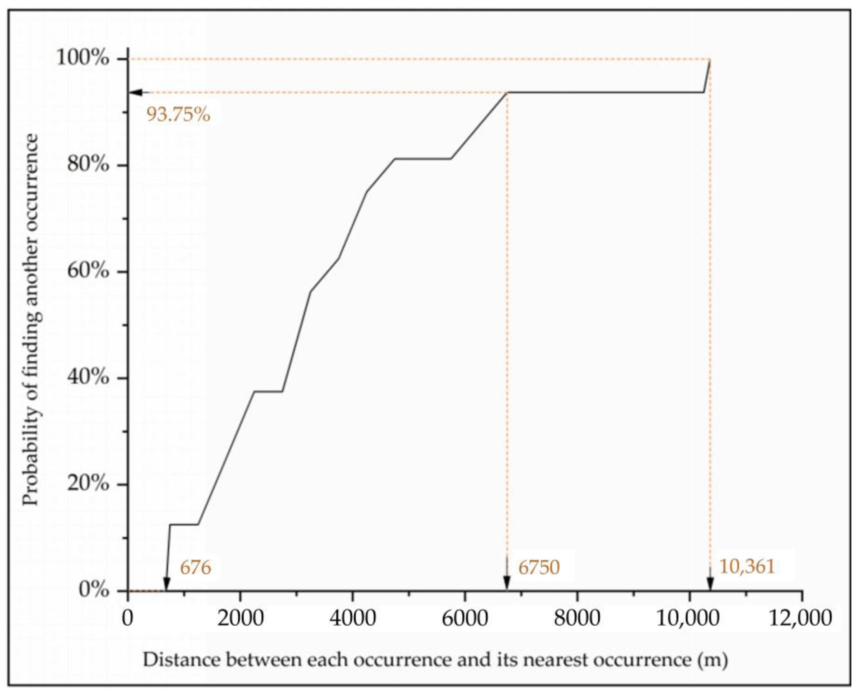
Before establishing a predictive model, it is necessary to convert all kinds of data containing evidence features into raster maps and build a suitable size cell grid in GIS to load this evidence feature data as predictive units. According to the method proposed by Carranza [68], the appropriate cell mesh size can be determined based on the objective situation. On the one hand, since occurrence are rare events in the region, it is necessary to ensure that one cell grid can contain at most one occurrence. According to proximity analysis, the minimum distance between any two occurrences in the study area can be calculated to be 676 m (Figure 7), which indicates that if a cell grid larger than this size is selected, there may be more than one occurrence in one cell grid, so 676 m can be used as the upper limit of cell grid size. On the other hand, based on the maximum scale of the evidence map, a lower limit of the cell grid size can be determined, which can be estimated by the following empirical formula [69]:

$$R_s=M_s\times 0.00025$$

(14)

where $R_s$ denotes the lower limit cell grid size and $M_s$ signifies the map scale. In this study, the minimum scale of the evidence map is 1:250,000, so the lower limit of the cell grid can be determined to be 62.5 m. According to the upper and lower limits, a grid with a size of 500 m was selected to generate a raster map containing 27,925 cells, and each cell contained 10 evidence layers of geology, geophysics, geochemistry and remote sensing.

The dataset used for training ML models should contain samples with positive and negative labels, in which the cells with occurrence are labeled as positive samples, and the cells with non-occurrence are labeled as negative samples. Occurrence locations are derived from Dong [49], while non-occurrence locations can be selected according to the decision rules proposed by Carranza and Zuo [1] and Carranza [68], which should meet three conditions as follows, namely that (i) the negative samples should be far enough away from the known occurrence in the area to minimize their ore-bearing probabilities, (ii) it is important that the number of negative samples used in model training is equal to that of positive samples and (iii) the selection of negative samples should cover the entire study area roughly and fully satisfy the principle of randomness, ensuring that the spatial correlation between negative samples is small enough [70].

According to the distance between any two adjacent occurrences in the area, the probability of the nearest occurrence appearing within a certain range can be calculated by analyzing the proximity distance, and the relationship between the proximity distance and the probability of finding any adjacent occurrences can be obtained by statistical analysis. As shown in Figure 7, the maximum distance between any two mineral sites is 10,361 m, which indicates that potential occurrences are almost impossible to occur outside the 10,361 m buffer zone. Therefore, non-occurrences should be selected within this distance, but the options outside such a large buffer zone are too limited. Instead, the distance selected in this study was 6750 m since it can not only make the selection range of non-occurrences large enough but also ensure that there is a 93.75% probability that no other occurrences are included in the buffer zone.

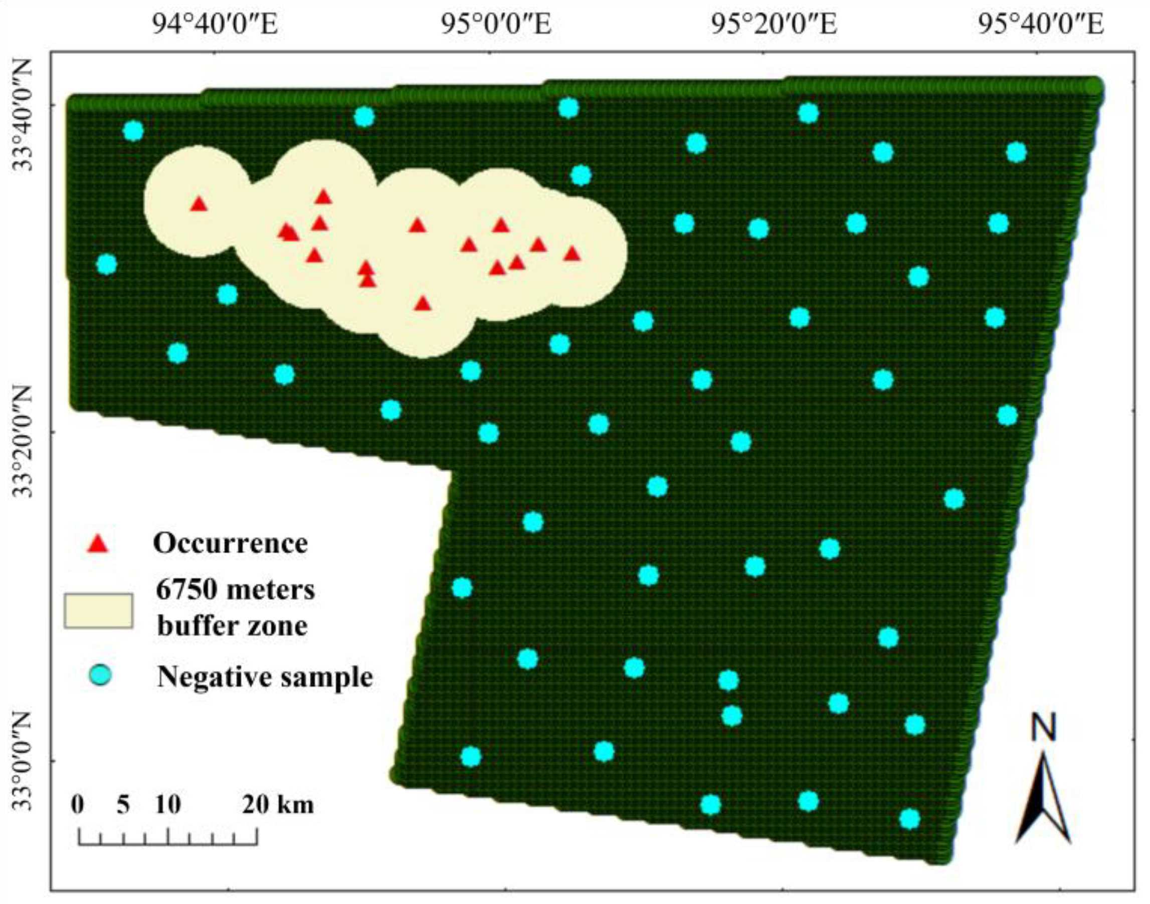
Based on the above criteria, 48 negative samples were selected in the study area (Figure 8). These samples were combined with 16 known occurrences to construct of a labeled dataset. SMOTE was then employed to augment the minority class to build a balanced dataset with equal numbers of positive and negative samples.

3.5.2. Parameter Optimization

Optimization of model parameters is one of the most important ways to improve the predictive performance of ML models. However, since there is still no general rule for determining the optimal parameters of the model in the field of ML, it is difficult to assign a prior reasonable parameter to a model. Consequently, it is necessary to fine-tune the sensitive parameters of the models to determine the optimal parameters of the models. In this study, the dataset was initially divided into a training set and a testing set according to a ratio of 7:3. Then the optimal parameter combination of four models’ training sets was obtained by means of K-fold cross-validation, which alleviates the overfitting problem that may be caused by dividing the training dataset at one time and enhances the generalization ability of the model. In this study, a $K$ value of 5 was adopted, leading to the random partitioning of the input training set data into five subsets of equivalent size. Among these, one subset was designated for validation purposes, while the remaining four subsets were employed for the model training. This process was repeated five times until each subset was used as a validation set once.

The mean square error (MSE) was employed to evaluate the results of cross-validation, which can be formulized as follows:

$$MSE={\displaystyle \frac{1}{N_t}}\sum _{i=1}^{N_t}{{(\widehat{y}}_i-y_i)}^2$$

(15)

where $N_t$ represents the number of data in validation dataset, ${\widehat{y}}_i$ denotes the predicted class value of target data (i.e., 1 for occurrence and 0 for non-occurrence) and $y_i$ signifies the true class value of target data. The model configuration with the lowest MSE was determined as the optimal one.

3.5.3. Performance Metrics

The classification performance of the prediction model can be evaluated by a fundamental term in ML named confusion matrix [71], in which there are four situations for a sample classified by the ML model, namely that (i) a sample that is actually an occurrence is correctly classified as an occurrence (called true positive sample or TP), (ii) a sample that is actually an occurrence is misclassified as a non-occurrence (called false negative sample or FN), (iii) a sample that is actually a non-occurrence is misclassified as an occurrence (called false positive sample or FP) and (iv) a sample that is actually non-occurrence is correctly classified as non-occurrence (called true negative sample or TN). A series of relevant evaluation indices can be calculated to evaluate the classification performance of the model, which can be expressed by the following formula [72,73]:

$$Sensitivity={\displaystyle \frac{TP}{TP+FN}}$$

(16)

$$Specificity={\displaystyle \frac{TN}{TN+FP}}$$

(17)

$$Positive predictive value={\displaystyle \frac{TP}{TP+FP}}$$

(18)

$$Negative predictive value={\displaystyle \frac{TN}{TN+FN}}$$

(19)

$$Accuracy={\displaystyle \frac{TP+TN}{TP+TN+FP+FN}}$$

(20)

Kappa measures the stability of the model by calculating the proportion of samples that are correctly classified after removing the probability of accidental agreement [74]. It can be expressed by the following formula [75,76]:

$$Kappa={\displaystyle \frac{TP+TN-\frac{\left(TP+FN\right)\left(TP+FP\right)+\left(TN+FN\right)\left(TN+FP\right)}{(TP+TN+FP+FN)}}{(TP+TN+FP+FN)-\frac{\left(TP+FN\right)\left(TP+FP\right)+\left(TN+FN\right)\left(TN+FP\right)}{(TP+TN+FP+FN)}}}$$

(21)

4. Results

4.1. Extraction of Ore-Related Alteration

According to classical alteration model of the study area (Figure 2), the target alterations to be extracted include potassic alteration, beresitization and propylitization. Since no potassic zones are found in the surface alteration, it is difficult to obtain the information of the potassic zone directly by remote sensing. Therefore, only the minerals related to the beresitization and propylitization were taken into consideration in the interpretation of remote sensing. Based on the ASTER proven spectral response bands of indicator minerals [35,77], indicator minerals, including jarosite, sericite, quartz, chlorite and epidote, were selected to trace alteration zones of pyritization, sericitization, silicification, chloritization and propylitization, respectively. Their corresponding spectral curves in the USGS spectral library are shown in Figure 9.

The principal component can be determined based on the spectral characteristics of the indicator minerals [77]. The feature vectors for indicator minerals of the PCA result were shown in

Table 1. Eigenvectors for indicator minerals, including jarosite, sericite, quartz, chlorite and epidote, with PCA based on ASTER data. The bold components represent the most suitable ones that are employed in the subsequent alteration extraction.

Indicator Mineral		PC1	PC2	PC3	PC4
Jarosite	Band 1	0.515831	0.569512	0.577487	0.275831
	Band 2	0.319782	0.233001	−0.078361	−0.915046
	Band 3	0.422136	0.294178	−0.806408	0.291489
	Band 4	0.673394	−0.731318	0.100368	0.040519
Sericite	Band 1	−0.242607	−0.625232	−0.538723	−0.509906
	Band 4	−0.960974	0.257465	0.089807	0.04664
	Band 6	0.129648	0.668019	−0.156013	−0.715962
	Band 7	0.029366	0.310719	−0.823026	0.474573
Quartz	Band 2	0.51378	0.584924	0.47045	0.415417
	Band 3	0.534755	0.351563	−0.618517	−0.455935
	Band 4	0.583442	−0.664527	−0.188246	0.427273
	Band 6	−0.331152	0.30442	−0.600564	0.661052
Chlorite	Band 1	−0.606167	−0.664767	−0.311625	−0.305838
	Band 2	−0.342449	−0.276984	0.664372	0.603837
	Band 5	0.030428	−0.0503	−0.674316	0.736099
	Band 8	−0.717192	0.691979	−0.082453	0.001399
Epidote	Band 1	−0.538364	−0.648355	−0.388355	−0.372802
	Band 3	−0.490353	−0.278288	0.612255	0.554304
	Band 5	−0.684097	0.708246	−0.091745	−0.148262
	Band 8	−0.041582	0.024072	−0.682574	0.729235

, and the spectrum curves of indicator minerals were depicted in Figure 9. According to Figure 9a, the spectrum curves of band 1 and band 3 show the characteristics of strong absorption, while band 2 and band 4 show reversely strong reflection. The band combination consisting of bands 1, 2, 3 and 4 was selected for the PCA of pyritization anomalies. In the resulting fourth principal component (PC4), the feature vectors for bands 1, 3 and band 2 exhibit opposite signs with large absolute values, aligning with the basic judgment rule described above. It is perfect that band 4 is negative, but it is also acceptable due to the value of 0.040519 that is close to the negative value. Therefore, the PC4 was selected as the identification result of pyritization anomalies. Similarly, the spectral curves of sericite in the bands 6 and 7 show strong absorption and reflection (Figure 9b), respectively. The band combination consisting of bands 1, 4, 6 and 7 was selected for PCA. In the resulting PC4, bands 6 and 7 have opposite sign and larger absolute value, so the PC4 was selected to represent the sericitization anomalies. The band spectral curve of quartz shows strong absorption characteristics in bands 2 and 6 (Figure 9c) and strong reflection in band 3 and band 4. The band combination, including bands 2, 3, 4 and 6, was selected, and the resulting third principal component (PC3) has the same symbol of bands 2 and 6, so the PC3 was selected to represent the silicification anomalies. Similarly, the band combination of 1, 2, 5 and 8 was selected for chloritization anomalies, and the PC4 was selected to represent chloritization anomalies. The epidote band combination of bands 1, 3, 5 and 8 was selected, and the PC4 was selected to represent the propylitization anomalies. The principal components of the five indicator minerals were obtained (Figure 10), which represents the zones where pyritization, sericitization, silicification, chloritization and propylitization are located, respectively. These features can be used as the predictor variables for ML-based MPM. Finally, ten multi-source features serve as input predictive variable fed into ML models, namely distance to porphyry intrusions, distance to regional faults, distance to ring structure, aeromagnetic anomalies, multivariate geochemical anomalies, silicification, sericitization, propylitization, chloritization and pyritization.

4.2. Performance Evaluation

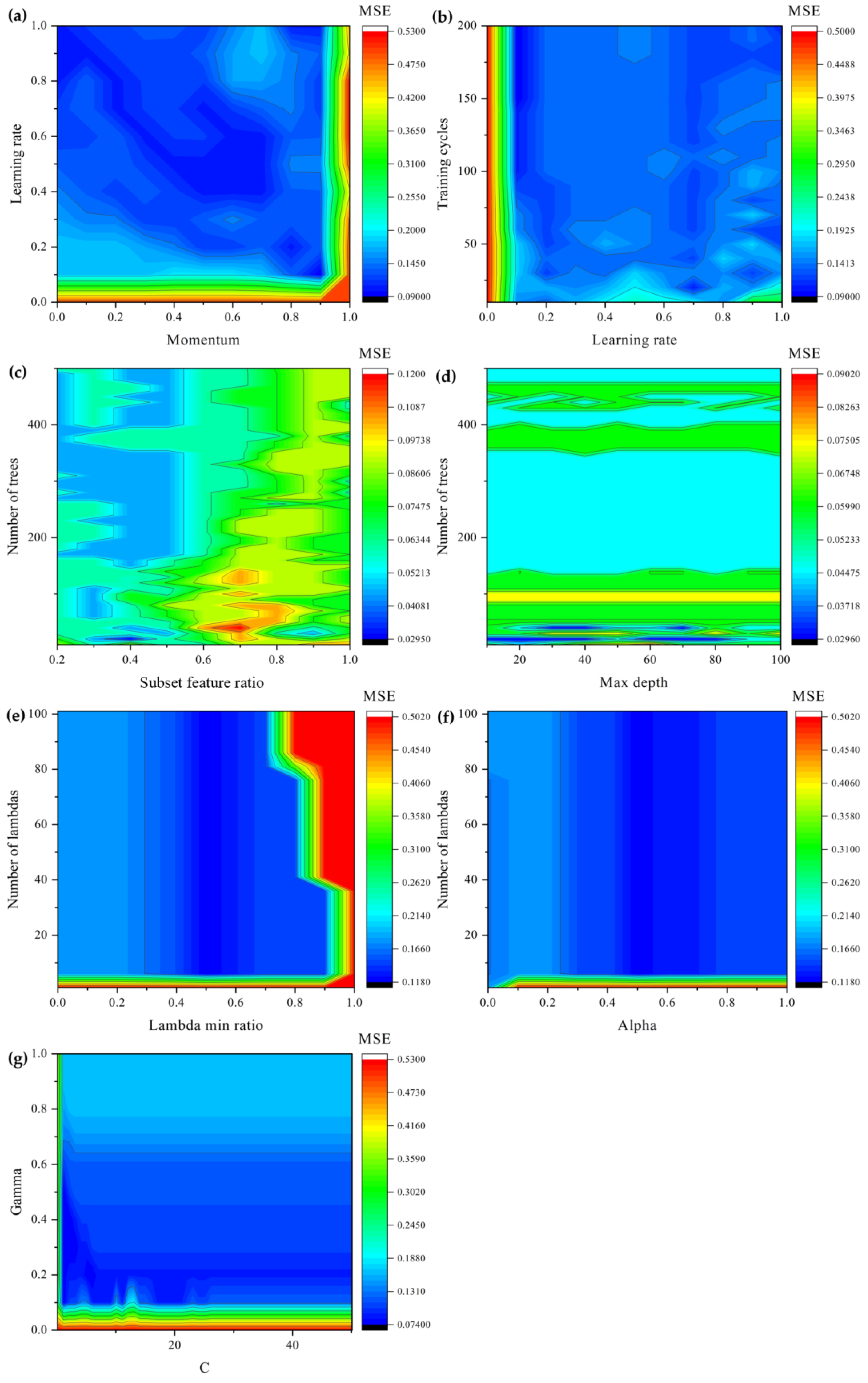
In the process of model training, the optimal parameters were determined by the strategy of grid search, i.e., the possible parameter combinations were exhaustively tested within a grid, where each cell represents a unique combination of parameters.

Table 2. Parameters used for training ML models.

Model	Parameter	Description	Reference Range	Optimal Parameter
ANN	Training cycles	Number of training cycles	10–200	200
	Learning rate	Change rate of weight in the training process	0–1	0.1
	Momentum	Prevent local maxima and smooth optimization directions	0–1	0.9
RF	Number of trees	Number of trees	10–510	40
	Subset features ratio	Ratio of randomly chosen features for training	0.2–1	0.4
	Maximum depth	Restrict the depth for each random tree	10–100	60
SVM	Gamma	A width parameter of radial basis function that determines the influencing range of each support vector	0–1	0.2
	Cost	Penalty factor for misclassification error	0.1–50.1	5.1
LR	Number of lambdas	Number of lambda values	1–101	26
	Lambda min ratio	Smallest value for lambda as a fraction of lambda	0–1	0.5
	Alpha	Controls the distribution between the L1 (Lasso) and L2 (Ridge regression) penalties	0–1	0.5

lists the reference ranges of parameter values of the employed four models suggested by previous studies [16,17]. The efficacy of a specific parameter combination was evaluated by MSE derived from 5-fold cross-validation, as mentioned in Section 3.5.2. Figure 11 illustrates the dynamic variation of MSE along with parameter changes. The parameters used to train the model with the lowest MSE were selected as the optimal parameters, which were listed in Table 2.

The different parameter configurations employed in model training significantly impact on the robustness and generalization capability of the machine learning methods. As presented in Figure 11, the fluctuation in the model’s classification error across diverse parameter settings and input datasets can be observed. Specifically, in the ANN model, both a low learning rate (<0.1) and a large momentum (>0.9) lead to an increase in MSE (Figure 11a). Under the condition of sufficient learning rate, increase in training cycle leads to slight and stable decrease in MSE (Figure 11b). In the RF model, increasing the number of trees generally reduces the MSE of the model, but such reduction is not evident (Figure 11c,d). The lowest MSEs are observed in the zones with a tree number smaller than 50. An increase in the tree number does not result in a significant decrease in MSE. The increase in the subset feature ratio participating in training will lead to the elevation of MSE. This increase effect is more obvious when a smaller number of trees is counted (< 150), which may be due to the poor generalization capability of the model caused by insufficient diversity. The variation of maximum depth has no significant effect on MSE. In the LR model, the low regularization strength (lambda < 5) induces severe inaccuracy (Figure 11e,f), while the varying lambdas exhibit a weak effect on MSE when its value exceeds 5. Additionally, the increase in the minimum ratio of lambda will lead to the increase in MSE, and the increase rate of MSE is significantly steeper when the lambda minimum ratio is greater than 0.7 (Figure 11e). In the SVM model, the value range of [0, 0.1] for gamma is warning for its resulting high MSE, while the variation in gamma and C in other zones is not sensitive to MSE (Figure 11g).

As shown in

Table 3. Statistical results of MSE calculated from 5-fold cross-validation.

Model	Mean Square Error
	Minimum	Maximum	Mean	Standard Deviation
ANN	0.009	0.53	0.2047	0.1368
RF	0.0295	0.121	0.0675	0.1773
SVM	0.074	0.53	0.169	0.1209
LR	0.118	0.502	0.2244	0.135

, among all the ML parameters, the RF model has the lowest average MSE of approximately 0.0675, followed by the average MSE of the SVM model with 0.169. In contrast, both the ANN and LR models exhibit higher average MSEs at 0.2047 and 0.2244, respectively. This indicates that the RF model exhibits the least error between its predicted values and the actual outcomes. The SVM model exhibits the smallest standard deviation in the 5-fold cross-validation, suggesting the model has the least variability across different parameter combinations. This indicates that the SVM model is less sensitive to changes in its parameters, which may be attributed to the fact that only two parameters are involved in the processes of parameter optimization.

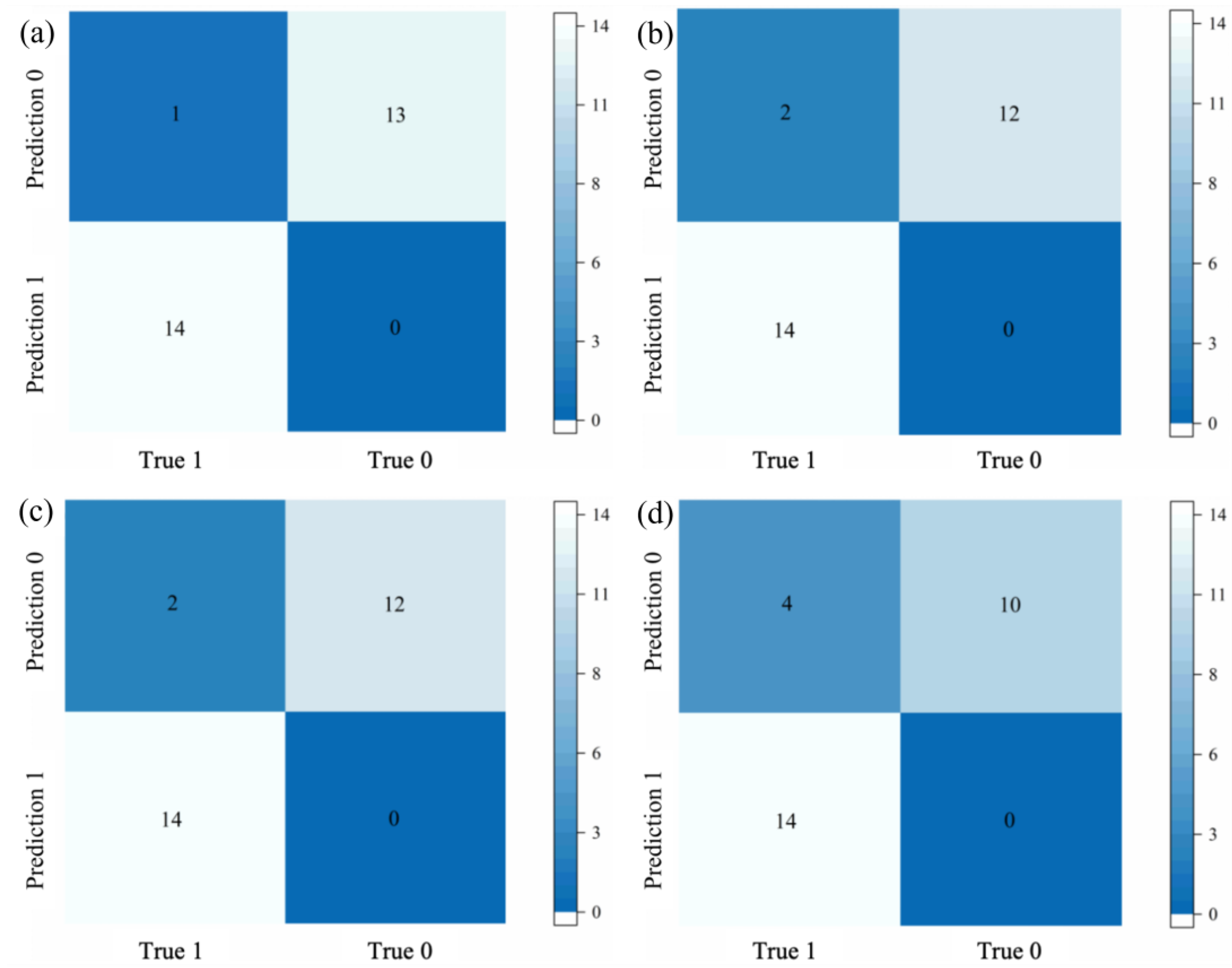
The prediction at each cell is represented by a floating probability value ranging from 0 to 1, which denotes the probability of a mineral occurrence. The ML algorithms label the cells with probability values greater than 0.5 as prospective areas, while the other cells are labeled as barren areas. The confusion matrices of the four models in the test dataset are shown in Figure 12, and various evaluation indices (

Table 4. Predictive performance of ML models.

Indices	ANN	RF	SVM	LR
Sensitivity	100.00%	100.00%	100.00%	100.00%
Specificity	93.33%	87.50%	87.50%	77.78%
Positive predict value	92.86%	85.71%	85.71%	71.43%
Negative predict value	100.00%	100.00%	100.00%	100.00%
Accuracy	96.43%	92.86%	92.86%	85.71%
Kappa	92.86%	85.71%	85.71%	71.43%

) are obtained from the calculation of the confusion matrices. In general, the ANN model achieves the greatest performance both in the overall accuracy and in predicting positive and negative samples, followed by the RF and SVM models, whereas the LR model produces relatively worse predictions. Specifically, all four models exhibit a sensitivity of 100%, confirming that they accurately identified all occurrence cells in the dataset. The ANN model exhibits a specificity of 93.33%, indicating that 93.33% of non-occurrence cells are correctly classified as barren areas. The rest of the models also achieved satisfactory values of specificity, with both RF and SVM reaching 87.5% and LR reaching 77.78%. The ANN model exhibits the most positive predictive value of 92.86%, indicating that 92.86% of the predicted prospective cells actually contain Cu-polymetallic occurrences, followed by both RF and SVM models, with 85.71%. The positive predictive value of the LR model is the lowest, which is 71.43%. The four models all have high negative predictive values, reaching 100%, indicating that 100% of predicted non-occurrence cells are true non-occurrence locations. The ANN model achieves the highest overall accuracy of 96.43%, indicating 96.43% of all samples are correctly classified, followed by the RF and SVM (92.86%) models and LR (85.71%) model, which produce relatively low value of classification accuracy. It can be observed that there are significant differences among the Kappa indices of the four models. The ANN model has the highest Kappa index value of 92.86%, followed by both RF and SVM models with the values of 85.71%, which indicates excellent agreement between the predictive models and observed mineral occurrences. The LR model, however, has a relatively low Kappa index value of 71.43%, reflecting a weaker correlation between the predictions and reality.

4.3. The Predictive Efficiency of Models

The success-rate curve provides a clear illustration of the predictive efficiency of the models by depicting the relationship between the target regions predicted by the models and the number of actual occurrences appearing in the area. The slope of the success-rate curve indicates the predictive efficiency of the model. In other words, the steeper the slope of the success-rate curve, the more occurrences are captured in a smaller delineated area. Based on this, the high-, moderate- and low-potential regions of Cu-polymetallic occurrences can be divided according to the thresholds identified by the intersection of the regression lines. The high-potential regions, commonly with a success-rate curve slope exceeding 5, are prospective areas suitable for further exploration [17]. The slope of the first segment of the success-rate curve, which denotes the high-potential regions, deems it as an indicator of predictive efficiency of the ML model that needs to be paid attention to in practical explorations. As shown in Figure 13, the first section of the success-rate curve of the RF model has the highest slope of 23.02, delineating the high-potential regions that cover only 3.5% of the total area but capture 75% of existing occurrences. The SVM model comes in second with the slope value of 10.473, capturing 56.25% of existing occurrences covering 4.8% of the total area. The LR and ANN models demonstrate relatively low predictive efficiency in the high-potential area, with slopes of 9.1114 and 6.3706, respectively.

Although ANN has the best performance in terms of model classification accuracy, in practical mineral exploration, it is more important to meet the requirement of a high success rate and limited target region that reduces exploration cost. Therefore, the predictive efficiency of high-potential areas should be ranked first. RF has the highest predictive efficiency with its predictive ability, and its classification accuracy also reaches a satisfactory level. Consequently, the RF model is considered the optimal model for exploration targeting in this area.

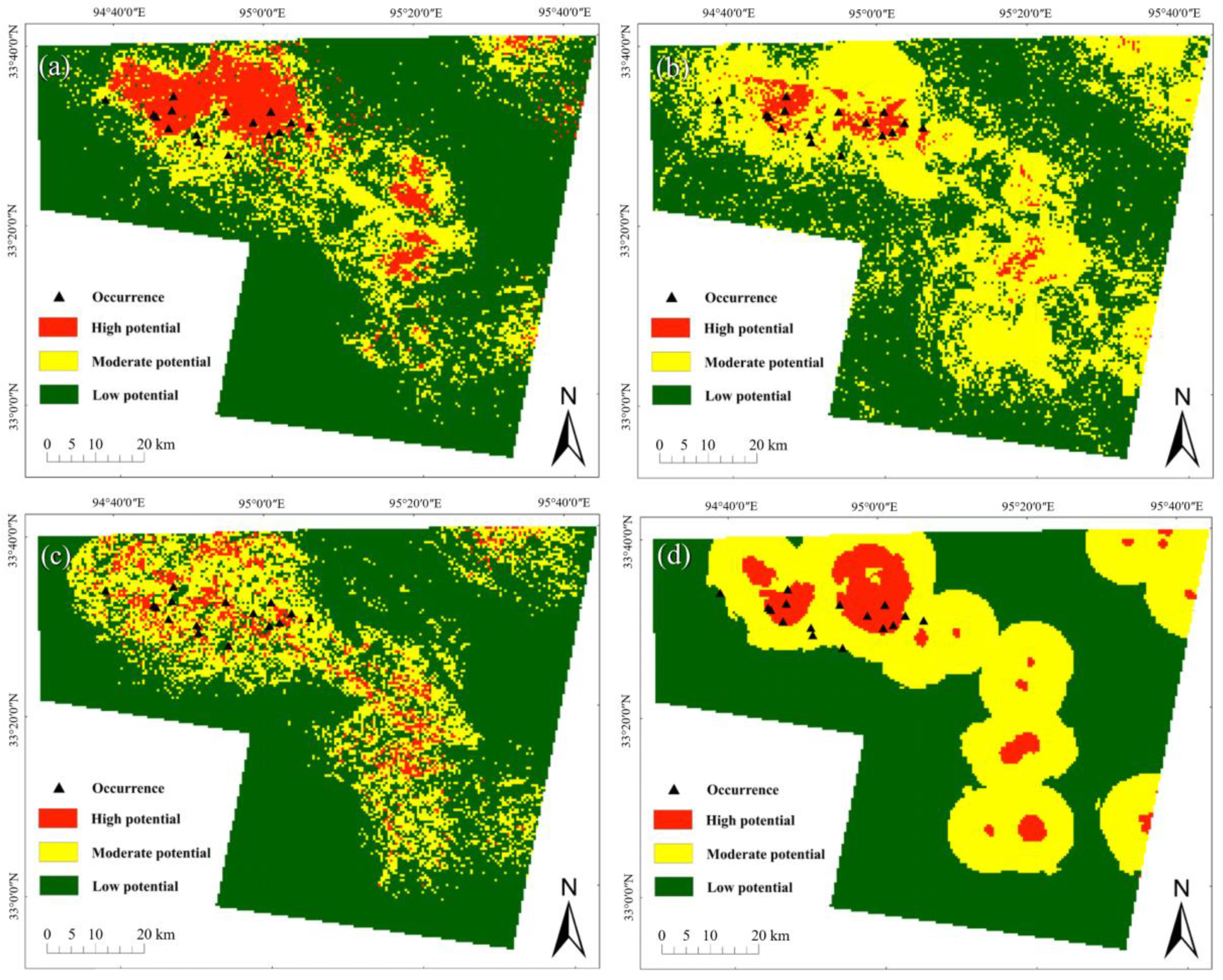
Based on the success-rate curves of the four models, the study area was subdivided into the high-, moderate- and low-potential regions, respectively, as shown in Figure 14. It can be found that the high-potential regions of the four models are mainly concentrated in Narigongma and Lurige mining areas, showing a strong correlation with the known occurrences. In the middle and north-east of the study area, there are also several small high-potential regions, but there are no known Cu-polymetallic occurrences in these regions, where further mineral exploration is strongly suggested to be implemented to probe their mineral potential.

4.4. Delineation of Exploration Targets

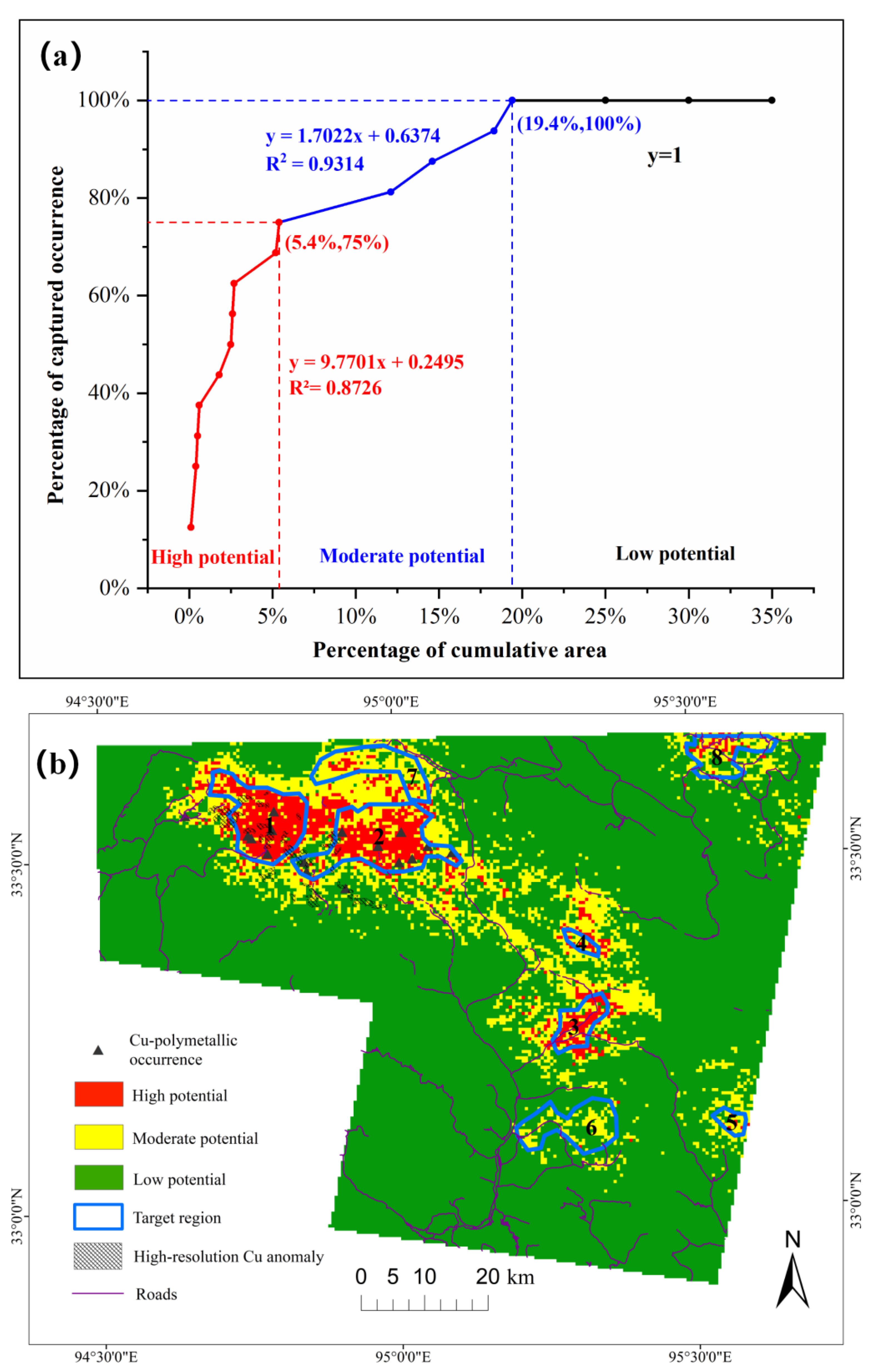
All the ML models described above can accurately classify positive and negative samples and draw high-potential areas with certain prediction efficiency. However, in order to meet the requirements of a high success rate and low risk in practical mineral exploration, the integration of multiple machine learning models was conducted to reduce the uncertainty of predictive results and improve the reliability of resultant exploration targets. For this purpose, the average predictive probability of four models in each cell was calculated and was employed to derived the success-rate curves (Figure 15a), based on which the final prospectivity map with high, moderate and low potential was generated (Figure 15b).

Eight regions of exploration target were delineated in the prospectivity map. Combined with the spatial analysis of multi-source evidential features, it can be found that all the target regions are located near the intrusions, within a buffered distance of 5600 m proximal to the intrusions, which reflects the strong correlation between intrusions and porphyry mineralization (Figure 16a). Targets 1# and 2# are located in the area of high multivariate geochemical anomaly, with an anomaly score greater than 5 (Figure 16b). As shown in Figure 16c, except for the Target 4#, the other target regions contain fault structures. Meanwhile, there are intersection points of fault structures in different directions in Targets 2#, 3#, 6# and 8#, and there is a certain probability of a mineralization center. The alteration zoning of the porphyry system has a typical concentric ring structure [78]. The spatial superposition of various alterations may indicate the existence of mineral deposits. As depicted from Figure 16d–h with medium-high alteration values, although a small portion of these targets overlaps with areas of lower alteration values. A comparative analysis of target region prospects is shown in detail in

Table 5. Comparative analysis of target regions.

No	Proportion of Target Region (%)	Number of Known Occurrences Included	Metallogenic Advantage
1#	1.83	5	(i) Large intrusions are exposed; (ii) most of the geochemical anomalies in the target regions were in the high-value area; (iii) existence of fault structure and intersection; (iv) high-value area of 4 kinds of alteration
2#	2.35	9	(i) Large intrusions are exposed; (ii) most of the geochemical anomalies in the target regions were in the high-value area; (iii) existence of fault structure and intersection; (iv) high-value area of 5 kinds of alteration
3#	0.62	0	(i) A small amount of intrusion is exposed; (ii) Existence of fault structure and intersection
4#	0.16	0	A small amount of intrusion is exposed
5#	0.2	0	A small amount of intrusion is exposed
6#	1.2	0	(i) A small amount of intrusion is exposed; (ii) existence of fault structure and intersection; (iii) high-value area of 2 kinds of alteration
7#	1.07	0	(i) A small amount of intrusion is exposed; (ii) existence of fault structure and intersection; (iii) high-value area of 3 kinds of alteration
8#	0.81	0	(i) A small amount of intrusion is exposed; (ii) existence of fault structure and intersection

. In order to validate the exploration targets, we employed high-resolution Cu anomalies derived from a 1:50,000 stream sediment geochemical survey [47], which can provide more accurate pathfinder information compared with the integrated geochemical anomalies from 1:200,000 data, although the mapping range of this survey is confined to the top-left corner of the study area that includes Targets 1#, 2# and 7#. A total of 321 samples were collected to quantitatively analyze nine mineralization-related elements, mainly using analytical methods of inductively coupled plasma mass spectrometry and X-ray fluorescence. However, only Cu anomalies were employed here for validating predictive targets. It can be observed from Figure 15b that all the Cu anomalies fall into the 1# and 2# high-potential areas and their surrounding moderate-potential zones. We also imported the road network to evaluate the transportation condition of the targets (Figure 15b). Based on comprehensive evaluation, Targets 1# and 3# are assigned the highest priority since Target 1# is validated by existing mineral occurrences and high-resolution geochemical anomalies with an accessible road condition, while Target 3# has superior transportation conditions and numerous high-potential zones. Although no mineral occurrences have been discovered yet, it holds significant potential for new discoveries of mineralization. Target 2# is supported by evidence of mineral occurrences and geochemical anomalies but has inconvenient transportation, placing it at a slightly lower exploration priority. Target 7# lacks validation from high-resolution geochemical anomalies but contains several high-potential units and a complete transportation network, while Target 8# has a well-developed transportation system and high-potential units. These targets can serve as third-tier alternatives. Among the remaining areas, Target 4# possesses high-potential units but lacks transportation access, and Targets 5# and 6# have transportation infrastructure but lack high-potential zones, rendering them the lowest-priority areas for exploration.

4.5. Model Interpretation

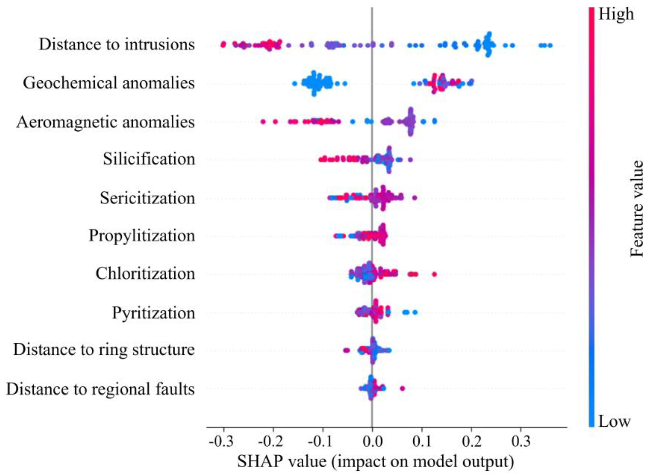
Machine learning algorithms have an inherent black-box effect, which precludes them from offering transparent modeling processes suitable for explaining their predictions. In this study, the Shapley additive explanation (SHAP) approach was employed to explain the output of RF models, which were found to be optimal models after model assessment. As shown in Figure 17, the points representing various values of sericitization anomalies, propylitization anomalies, distance to ring structures, and distance to regional faults are grouped within the SHAP range of [−0.1, 0.1] for sericitization anomalies, [−0.8, 0.3] for propylitization anomalies, [−0.5, 0.4] for distance to ring structures, and [−0.2, 0.6] for distance to regional faults. This clustering suggests that both high and low values of these features make similarly weak contributions to the model’s output. In contrast, the distance to intrusions and geochemical anomaly show a wide scatter distribution in their ratio. Most of the blue dots’ distance to intrusions are distributed on the positive axis of the SHAP scatter plot, which indicates that the closer the distance to the intrusions related to mineralization is, the stronger the ability of the model is to predict positive samples. Certain remote sensing features, including pyritization anomalies, sericitization anomalies and silicification anomalies, exhibit an opposite relationship with their SHAP values. This is due to the fact that during the PCA of these alterations, the actual mineralization information must be inverted to align with the principal component identified through remote sensing. However, this inversion does not impact the model’s learning of the mineralization pattern.

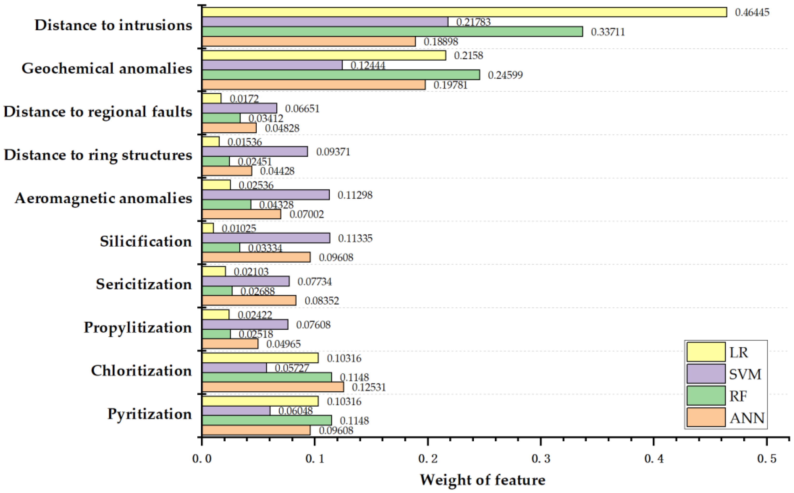
The geological interpretation of ML models can be conducted by analyzing the relative importance of each feature to the models’ predicted results, which can be calculated by the information gain ratio. As shown in Figure 18, the individual features exert distinctly varying importance in different ML models. Basically, LR and RF models exhibits more contrasting weights among different features, whereas SVM and ANN show more balanced weights. Specifically, the distance to intrusions has the highest relative importance among the three models of RF, SVM and LR models and ranks the second in ANN model. This is because the porphyry intrusions serve as the source of both energy and ore-forming materials, thus considered as the most ore-controlling factor within the geological understanding of mineral system in this area. The Cu-Mo-W-Co-Ni-Fe-Mn multivariate geochemical anomaly is the most important feature in ANN model, and the second most important feature in RF, SVM and LR models, which emphasizes the validity of geochemical indicators in tracing the mineralization in this area. Among the four models, the weights of pyritization, chloritization and silicification anomalies are only inferior to those of the distance to the intrusions and geochemical anomalies. In the known deposits such as the Narigongma deposit and Lurige deposit of the area, ore-bearing porphyry intrusions intruded into the intermediate-basic volcanic rocks, resulting in widespread well-developed pyritization, silicification and chloritization [37]. The relatively high contributions of these alteration features on model predictions demonstrates the effectiveness of employed remote sensing information for tracing the mineralization-related spatial proxies. In this study, the overall relative importance of remote sensing data in the ANN, RF and SVM models is considerable, with percentages of 45.06%, 31.5% and 38.45%, respectively. This suggests that a remote sensing interpretation can be a significant data source for MPM, particularly in greenfield areas that are less explored.

5. Discussion

5.1. Robust Framework of ML-Based MPM in Under-Explored Areas

ML algorithms have demonstrated their excellent predictive performance in mature, data-rich mining districts [7,16,17]. However, a new pressing challenge emerges in current mineral exploration tasks, that is, easily accessible mineral resources located in convenient-conditional, well-explored areas have largely been exhausted. The exploration foci are transferring to those areas characterized by harsh conditions and low exploration extent. Conducting ML-based MPM in such areas is highly challenging, yet critically necessary. The Narigongma area, serving as a typical under-explored region, is located at high altitudes with harsh natural conditions, where conventional geological exploration efforts are difficult to carry out, resulting in scarce data available for MPM. Therefore, this study focused on investigating robust frameworks for implementing ML-based MPM in under-explored areas. To achieve this goal and to address inherent issues involved in ML-based MPM, we employed effective scenarios in pre-modeling processing, predictive modeling and post-modeling assessment and application.

During the pre-modeling phase, data scarcity, including both insufficient evidence layers and limited mineral occurrences, is pivotal for robust MPM in under-explored regions. To address the lack of evidential layers, since the target deposits in this area developed distinct alteration zoning (Figure 2), we extracted five types of hydrothermal alteration related to porphyry mineralization via remote sensing (Figure 10), which enriched the input features used for model prediction. The sparse vegetation coverage in the study area also encourages the implementation of remote sensing-based alteration extraction. The results of the feature importance analysis (Figure 18) revealed that although remote sensing layers could not exert the most prominent influences on model output as those geological evidences did, they contributed considerably to the model prediction. Pyritization and chloritization related to beresitization especially exhibited substantial contributions to predictions, only inferior to the well-identified ore-controlling factors of intrusions and geochemical anomalies. This interpretable result aligns with established geological knowledge presented in Section 2, validating the effectiveness of integrating remote sensing features in mitigating data scarcity challenges. For the latter issue of scarce mineral occurrences, we leveraged SMOTE to generate synthetic training samples for model training. This data augmentation technique showcased its proven efficacy and broad applicability in the MPM domain in the recent literature [26,28]. The results of previous study indicated the SMOTE-augmented dataset consisting of balanced positive and negative samples generalized better model performance [28], which is due to the fact that SMOTE-ed data increases the decision boundary difference between positive and negative samples, suggesting a broader decision width and boosting the recognition ability of the ML models that favored more accurate classification [26].

In the process of predictive modeling, we employed a rigorous strategy combining a grid search with five-fold cross-validation to ensure the robustness of the parameter optimization for the four models. As shown in Figure 11, the results of model training indicate that the parameter combinations exhibit strong randomness in the accuracy of resultant models when tackling few-shot data. In this regard, empirical parameter selection or error convergence strategy are unsuitable for MPM studies. The employed grid search strategy, as a “trial-and-error” method, is not theoretically optimal but proves to be the most effective for model training in this study.

During the phase of post-modeling assessment and application, based on comprehensive evaluation, we focused on two critical issues, namely exploration significance and the uncertainty of modeling results. Although the confusion matrix and its derivative metrics are extensively employed in machine learning evaluation, they employ a low probability threshold of 0.5 for discriminating mineralized versus barren units, which is not suitable for expensive-cost and high-risk mineral exploration tasks. In addition, these metrics solely measure algorithmic performance without incorporating domain-specific constraints or exploration principles. Consequently, we prioritized the success-rate curve as the primary evaluation criterion, which can reflect the core principle of mineral exploration, i.e., maximizing success-rate while minimizing the delimited area. Based on this criterion, we not only ranked ML models by their ability to achieve high predictive efficiency (Figure 13 and Figure 15a) but also delineated zones of different prospectivity levels from exploration significance (Figure 14 and Figure 15b). The interpretability analyses link the modeling results and geological background, providing clues for explaining the model performance. ANN showed the best performance when evaluated by the low-threshold confusion matrix (Table 4), whereas it exhibited relatively poor performance in the success-rate curve where the top probability threshold is measured (Figure 13a). This may be attributed to the fact that ANN model failed to capture the most significant mineralization information (i.e., intrusion and geochemical anomalies) in the decision-making process, with relatively lower weights in these features (Figure 18), which leads to its weak recognition ability for identifying the prospective targets when limited area (8.9%) was counted (Figure 13a). In comparison, RF achieved the best performance in predictive efficiency, not only because of its random mechanism that proved to have anti-overfitting ability in few-shot tasks [57] but also due to the fact that RF model perfectly distinguished the most important ore-controlling factors in its predictive modeling, evidenced by the key feature contributions of intrusions and geochemical anomalies as well as significant influences exerted by chloritization and pyritization anomalies (Figure 18), which accords well with our understanding of porphyry mineral systems, as we discussed before. Given the consistently satisfactory performance of all four models employed in this study, we integrated their predictions for delineating final exploration targets. Such a strategy can balance between optimality and stochasticity of individual models and can alleviate the uncertainty issue to some extent.

5.2. Limitation and Future Work

Although the ML-based MPM of this study achieved satisfactory results, there remain some limitations. Uncertainty represents a major constraint in this study. Geological exploration is inherently high-risk and highly uncertain, stemming from the extreme complexity of ore-forming systems and the noise information derived from the vast spatial-temporal evolution of geological processes. A key advantage of ML-based mineral prospectivity modeling lies in its powerful ability of pattern recognition for extracting mineralization-related information. Nevertheless, the raw data still contains substantial irrelevant noise signals unrelated to mineralization, which can mislead both geologists and ML models during the decision-making stage. Secondly, the black-box nature of ML modeling introduces uncontrollable uncertainty. To address this, the study implemented rigorous procedures of parameter optimization and post-modeling interpretability analyses to minimize uncertainty arising from this source. Finally, biases in understanding the mineral systems also induce uncertainty. As shown in the workflow presented in Section 5.1, the understanding of the porphyry mineral system guides both feature selection before modeling and interpretable application of predictive results after modeling. Deviations in geological understanding negatively impact these critical stages, increasing model uncertainty and reducing prediction efficacy.

The lack of advanced ML algorithms constitutes another limitation of this study. The machine learning algorithms are advancing rapidly, and some cutting-edge techniques such as deep forest [7] and graph-based neural networks [79,80] have been introduced and applied in the MPM domain. We initially considered adopting a deep learning algorithm with more complex architectures. However, given that the study area is a greenfield region restricted by data scarcity, training sophisticated models with limited data would likely lead to overfitting and bad generalization results, as reported in the previous literature [16,28]. Therefore, the employment of advanced machine learning algorithms in the future poses no significant technical hurdle, but the critical challenge lies in establishing a data-efficient environment to enable their effective implementation.

Future work should focus on expanding effective data sources, which would dilute irrelevant mineralization information and establish a data foundation for the application of advanced ML algorithms, as discussed above. Incorporating multi-source remote sensing data represents a promising direction, particularly through the introduction of high-resolution remote sensing data (e.g., WorldView-3, ZY1E hyperspectral imagery). These data offer higher characterization accuracy for specific alteration minerals, thereby enhancing the effectiveness of alteration extraction. Additionally, efforts should prioritize the expansion of the valid characterization of mineralization information. A novel framework of numerical terrain analysis integrating mineralogy, geomorphology, satellite imagery, ground-truthing, sedimentology and isotopic analysis has been recently proposed by Dill et al. [81,82,83]. The core of the method that inspires us is to build a genetic link between the geomorphological indices and complex geodynamic evolution of the target system (e.g., mineral system), allowing for tracing the hidden system behaviors (e.g., mineralization) via accessible quantitative indices. This method has been successfully applied in hot-spot island-related REE deposits [81,82]. In our case, given the highly exposed bedrock conditions in the study area, terrain indices derived from mineralogical–geomorphological analysis can also be effectively employed to trace specific mineralization-related alteration information, although these indices are less sensitive than in the studies of REE deposits. For example, rocks altered by propylitization (characterized by carbonatization and chloritization) are prone to weathering and erosion, often forming gentle slopes or depressions. In contrast, silicification exhibits strong resistance to weathering, typically forming raised alteration highlands or steep scarps. Pyrite near the surface oxidizes to form limonite (iron hat), resulting in a loosened rock structure that is easily eroded, commonly leading to depressions, gullies or negative topography. However, pyritization can be associated with silicification and structural fracture zones, which induces the formation of linear highlands. These landscape-specific alterations can be traced by the geomorphological indices, which contribute to enrich the evidential features for ML-based predictive modeling.

6. Conclusions

Mapping mineral potentials through advanced predictive models is crucial for mineral exploration activities, especially for exploration targeting in greenfield, where scarce data are available. In this study, ML-based MPM using four ML models, namely ANN, RF, SVM and LR, was employed to map the Cu-polymetallic prospectivity in Narigongma area. A remote sensing technique was employed to extract mineralization-related alteration, enriching the data source for MPM modeling. The dataset consists of 10 multi-source evidence layers, which provides a sound data basis for model training. The SMOTE method was utilized to balance the labeled dataset. To determine the optimal parameter combination for the model, a grid search strategy with 5-fold cross-validation was employed. The performance and efficiency of the models were evaluated by confusion matrices and success-rate curves. The results show that all four models have considerable predictive capability, among which ANN has the best classification accuracy, whereas RF achieves the highest predictive efficiency, which captures 75% of known occurrences in the 3.5% high-potential area. According to the comprehensive integration of the four ML models, eight prospecting target regions were delineated, and these regions align well with favorable geological conditions for ore formation. The exploration targets were finally ranked based on the verification of high-resolution geochemical anomalies and transportation conditions. The results of model interpretability analyses highlight the crucial influences exerted by spatial proxies of porphyry intrusions and geochemical exploration as well as significant contributions of pyritization and chloritization, which accords well with the established knowledge about porphyry mineral systems in the study area.

The findings of this study demonstrate that the ML models trained on remote sensing and multi-source information provide an effective solution for MPM in well-exposed and under-explored areas. The limitations of the study lie in uncertainties induced by multiple sources of data, model and knowledge as well as the lack of cutting-edge algorithms, which are partly rooted in data scarcity issues. Therefore, future work focuses on expanding effective data sources, which can be implemented by employing hyperspectral imagery and introducing new pathfinder indicators such as mineralogy-linked geomorphological indices.

References

1. Zuo, R.; Carranza, E.J.M. Support vector machine: A tool for mapping mineral prospectivity. Comput. Geosci. 2011, 37, 1967–1975. [Google Scholar] [CrossRef]
2. Porwal, A.; Carranza, E.J.M. Introduction to the special issue: GIS-based mineral potential modelling and geological data analyses for mineral exploration. Ore Geol. Rev. 2015, 71, 477–483. [Google Scholar] [CrossRef]
3. Chung, C.F.; Agterberg, F.P. Regression models for estimating mineral resources from geological map data. J. Int. Assoc. Math. Geol. 1980, 12, 473–488. [Google Scholar] [CrossRef]
4. Harris, J.R.; Sanborn-Barrie, M.; Panagapko, D.A.; Skulski, T.; Parker, J.R. Gold prospectivity maps of the Red Lake greenstone belt: Application of GIS technology. Can. J. Earth Sci. 2006, 43, 865–893. [Google Scholar] [CrossRef]
5. Agterberg, F.P. Combining indicator patterns in weights of evidence modeling for resource evaluation. Nat. Resour. Res. 1992, 1, 39–50. [Google Scholar] [CrossRef]
6. Carranza, E.J.M. Data-Driven Evidential Belief Modeling of Mineral Potential Using Few Prospects and Evidence with Missing Values. Nat. Resour. Res. 2015, 24, 291–304. [Google Scholar] [CrossRef]
7. Liu, Y.; Sun, T.; Wu, K.; Zhang, J.; Zhang, H.; Pu, W.; Liao, B. Tungsten prospectivity mapping using multi-source geo-information and deep forest algorithm. Ore Geol. Rev. 2025, 177, 106452. [Google Scholar] [CrossRef]
8. Qin, Y.; Liu, L.; Wu, W. Machine Learning-Based 3D Modeling of Mineral Prospectivity Mapping in the Anqing Orefield, Eastern China. Nat. Resour. Res. 2021, 30, 3099–3120. [Google Scholar] [CrossRef]
9. Forson, E.D.; Amponsah, P.O. Mineral prospectivity mapping over the gomoa area of Ghana’s southern kibi-winneba belt using support vector machine and naive bayes. J. Afr. Earth Sci. 2023, 206, 105024. [Google Scholar] [CrossRef]
10. Brown, W.M.; Gedeon, T.D.; Groves, D.I.; Barnes, R.G. Artificial neural networks: A new method for mineral prospectivity mapping. Aust. J. Earth Sci. 2000, 47, 757–770. [Google Scholar] [CrossRef]
11. Brown, W.M.; Gedeon, T.D.; Groves, D.I. Use of Noise to Augment Training Data: A Neural Network Method of Mineral-Potential Mapping in Regions of Limited Known Deposit Examples. Nat. Resour. Res. 2003, 12, 141–152. [Google Scholar] [CrossRef]
12. Sun, T.; Feng, M.; Pu, W.; Liu, Y.; Chen, F.; Zhang, H.; Huang, J.; Mao, L.; Wang, Z. Fractal-Based Multi-Criteria Feature Selection to Enhance Predictive Capability of AI-Driven Mineral Prospectivity Mapping. Fractal Fract. 2024, 8, 224. [Google Scholar] [CrossRef]
13. Abedi, M.; Norouzi, G.H.; Bahroudi, A. Support vector machine for multi-classification of mineral prospectivity areas. Comput. Geosci. 2012, 46, 272–283. [Google Scholar] [CrossRef]
14. Zheng, C.; Yuan, F.; Luo, X.; Li, X.; Liu, P.; Wen, M.; Chen, Z.; Albanese, S. Mineral prospectivity mapping based on Support vector machine and Random Forest algorithm – A case study from Ashele copper–zinc deposit, Xinjiang, NW China. Ore Geol. Rev. 2023, 159, 105567. [Google Scholar] [CrossRef]
15. Carranza, E.J.M.; Laborte, A.G. Random forest predictive modeling of mineral prospectivity with small number of prospects and data with missing values in Abra (Philippines). Comput. Geosci. 2015, 74, 60–70. [Google Scholar] [CrossRef]
16. Sun, T.; Chen, F.; Zhong, L.; Liu, W.; Wang, Y. GIS-based mineral prospectivity mapping using machine learning methods: A case study from Tongling ore district, eastern China. Ore Geol. Rev. 2019, 109, 26–49. [Google Scholar] [CrossRef]
17. Sun, T.; Li, H.; Wu, K.; Chen, F.; Zhu, Z.; Hu, Z. Data-driven predictive modelling of mineral prospectivity using machine learning and deep learning methods: A case study from Southern Jiangxi Province, China. Minerals 2020, 10, 102. [Google Scholar] [CrossRef]
18. Fu, Y.; Cheng, Q.; Jing, L.; Ye, B.; Fu, H. Mineral Prospectivity Mapping of Porphyry Copper Deposits Based on Remote Sensing Imagery and Geochemical Data in the Duolong Ore District, Tibet. Remote Sens. 2023, 15, 439. [Google Scholar] [CrossRef]
19. Carranza, E.J.M.; Ruitenbeek, F.J.A.V.; Hecker, C.A.; Meijde, M.V.D.; Meer, F.D.V.D. Knowledge-guided data-driven evidential belief modeling of mineral prospectivity in Cabo de Gata, SE Spain. Int. J. Appl. Earth. Obs. Geoinform. 2008, 10, 374–387. [Google Scholar] [CrossRef]
20. Carranza, E.J.M. Geocomputation of mineral exploration targets. Comput. Geosci. 2011, 37, 1907–1916. [Google Scholar] [CrossRef]
21. Cheng, Q. Mapping singularities with stream sediment geochemical data for prediction of undiscovered mineral deposits in Gejiu, Yunnan Province, China. Ore Geol. Rev. 2007, 32, 314–324. [Google Scholar] [CrossRef]
22. Cheng, Q. Singularity theory and methods for mapping geochemical anomalies caused by buried sources and for predicting undiscovered mineral deposits in covered areas. J. Geochem. Explor. 2012, 122, 55–70. [Google Scholar] [CrossRef]
23. Chawla, N.; Japkowicz, N.; Aleksander, K. Editorial: Special Issue on Learning from Imbalanced datasets. Sigkdd Explor. 2004, 6, 1–6. [Google Scholar] [CrossRef]
24. Hariharan, S.; Tirodkar, S.; Porwal, A.; Bhattacharya, A.; Joly, A. Random Forest-Based Prospectivity Modelling of Greenfield Terrains Using Sparse Deposit Data: An Example from the Tanami Region, Western Australia. Nat. Resour. Res. 2017, 26, 489–507. [Google Scholar] [CrossRef]
25. Fernandez, A.; Garcia, S.; Herrera, F. SMOTE for Learning from Imbalanced Data: Progress and Challenges, Marking the 15-year Anniversary. J. Artif. Intell. Res. 2018, 61, 863–905. [Google Scholar] [CrossRef]
26. Liu, Y.; Sun, T.; Wu, K.; Xiang, W.; Zhang, J.; Zhang, H.; Feng, M. Interpretability Analysis of Data Augmented Convolutional Neural Network in Mineral Prospectivity Mapping Using Black-Box Visualization Tools. Nat. Resour. Res. 2025, 34, 759–783. [Google Scholar] [CrossRef]
27. Li, T.; Xia, Q.; Zhao, M.; Gui, Z.; Leng, S. Prospectivity Mapping for Tungsten Polymetallic Mineral Resources, Nanling Metallogenic Belt, South China: Use of Random Forest Algorithm from a Perspective of Data Imbalance. Nat. Resour. Res. 2019, 29, 203–227. [Google Scholar] [CrossRef]
28. Zhou, K.; Sun, T.; Liu, Y.; Feng, M.; Tang, J.; Mao, L.; Pu, W.; Huang, J. Prospectivity Mapping of Tungsten Mineralization in Southern Jiangxi Province Using Few-Shot Learning. Minerals 2023, 13, 669. [Google Scholar] [CrossRef]
29. Sabins, F. Remote sensing for mineral exploration. Ore Geol. Rev. 1999, 14, 157–183. [Google Scholar] [CrossRef]
30. Mahmood, T.H.; Hasan, K.; Akhter, S.H. Lithologic mapping of a forested montane terrain from Landsat 5 TM image. Geocarto Int. 2019, 34, 750–768. [Google Scholar] [CrossRef]
31. Shirmard, H.; Farahbakhsh, E.; Müller, R.; Chandra, R. A review of machine learning in processing remote sensing data for mineral exploration. Remote Sens. Environ. 2022, 268, 112750. [Google Scholar] [CrossRef]
32. Mohamed Taha, A.M.; Xi, Y.; He, Q.; Hu, A.; Wang, S.; Liu, X. Investigating the Capabilities of Various Multispectral Remote Sensors Data to Map Mineral Prospectivity Based on Random Forest Predictive Model: A Case Study for Gold Deposits in Hamissana Area, NE Sudan. Minerals 2023, 13, 49. [Google Scholar] [CrossRef]
33. Eldosouky, A.M.; Abdelkareem, M.; Elkhateeb, S.O. Integration of remote sensing and aeromagnetic data for mapping structural features and hydrothermal alteration zones in Wadi Allaqi area, South Eastern Desert of Egypt. J. Afr. Earth. Sci. 2017, 130, 28–37. [Google Scholar] [CrossRef]
34. Francisco, T.; Cecilia, V.; David, C.; Zhang, L. Lithological and Hydrothermal Alteration Mapping of Epithermal, Porphyry and Tourmaline Breccia Districts in the Argentine Andes Using ASTER Imagery. Remote Sens. 2018, 10, 203. [Google Scholar]
35. Zhao, Z.; Zhou, J.; Lu, Y.; Chen, Q.; Cao, X.; He, X.; Fu, X.; Zeng, S.; Feng, W. Mapping alteration minerals in the Pulang porphyry copper ore district, SW China, using ASTER and WorldView-3 data: Implications for exploration targeting. Ore Geol. Rev. 2021, 134, 104171. [Google Scholar] [CrossRef]
36. Chen, Q.; Zhao, Z.; Zhou, J.; Zeng, M.; Xia, J.; Sun, T.; Zhao, X. New Insights into the Pulang Porphyry Copper Deposit in Southwest China: Indication of Alteration Minerals Detected Using ASTER and WorldView-3 Data. Remote Sens. 2021, 13, 2798. [Google Scholar] [CrossRef]
37. Yang, Z.; Hou, Z.; Xu, J.; Bian, X.; Wang, G.; Yang, Z.; Tian, S.; Liu, Y.; Wang, Z. Geology and origin of the post-collisional Narigongma porphyry Cu-Mo deposit, southern Qinghai, Tibet. Gondwana Res. 2014, 26, 536–556. [Google Scholar] [CrossRef]
38. Hou, Z.; Zeng, P.; Gao, Y.; Du, A.; Fu, D. Himalayan Cu–Mo–Au mineralization in the eastern Indo–Asian collision zone: Constraints from Re–Os dating of molybdenite. Miner. Deposit. 2006, 41, 33–45. [Google Scholar] [CrossRef]
39. Yin, A.; Harrison, T.M. Geologic evolution of the Himalayan-Tibetan orogen. Annu. Rev. Earth Pl. Sc. 2000, 28, 211–280. [Google Scholar] [CrossRef]
40. Wang, Z.; Yang, Z.; Yang, Z.; Tian, S.; Liu, Y.; Ma, Y.; Wang, G.; Qu, W. Narigongma porphery molybdenite copper deposit, northern extension of Yulong copper belt: Evidence from the age of Re-Os isotope. Acta Petrol Sin. 2008, 24, 503–510. [Google Scholar]
41. Song, Z.; Jia, Q.; Chen, X.; Chen, B.; Zhang, Y.; Zhang, X.; Quan, S.; Li, Y. The Petrogenic age of Narigongma Granitic Diorite-porphyry in the Northern Part of the Sanjiang region and Its geological implications. Acta Geosci. Sinica 2011, 32, 154–162, (In Chinese with English Abstract). [Google Scholar]
42. Song, Z.; Jia, Q.; Zhang, Y.; Chen, B.; Chen, X.; Wang, F.; Tian, Y.; Li, Y.; Zhang, X.; Quan, S. LA-ICPMS ziron U-Pb dating of Narigongma biotite granite porphyry in northern Sanjiang region and its geological significance. Geol. Bull. China 2012, 31, 439–447, (In Chinese with English Abstract). [Google Scholar]
43. Zhang, M.; Liu, J.; Xiao, W.; Yang, Z. Geological characteristics and ore prospecting orientation of porphyry copper deposit in Qinghai Province. Miner. Res. Geol. 2007, 21, 440–444. [Google Scholar]
44. GeoCloud Database of China Geological Survey. Available online: https://geocloud.cgs.gov.cn (accessed on 23 September 2025).
45. Hu, X.; Li, X.; Yuan, F.; Ord, A.; Jowitt, S.M.; Li, Y.; Dai, W.; Zhou, T. Numerical modeling of ore-forming processes within the Chating Cu-Au porphyry-type deposit, China: Implications for the longevity of hydrothermal systems and potential uses in mineral exploration. Ore Geol. Rev. 2020, 116, 103230. [Google Scholar] [CrossRef]
46. Chen, J.; Pan, T.; Hao, J. Metallogenic Regularity and Prediction of the Copper Polymetallic Deposit in the North Section of Sanjiang in Qinghai Province; Geological Publishing House: Beijing, China, 2010. (In Chinese) [Google Scholar]
47. Wang, F. Exploration model and periphery prospecting prediction for Narigongma porphyry copper-molybdenum deposit in the northern part of Sanjiang, Qinghai province. Master Thesis, Jilin University, Jilin, China, 2014. (In Chinese with English Abstract). [Google Scholar]
48. Zhang, J. Study on Extraction Method of Remote Sensing AlterationInformation in Yulong Porphyry Copper Belt. Master Thesis, Chengdu University of Technology, Sichuan, China, 2017. (In Chinese with English Abstract). [Google Scholar]
49. Dong, Q. Quantitative Evaluation and Prediction of Regional Metallogeny in Northern Segment of Three River Region, Southwest China. Ph.D. Thesis, China University of Geosciences, Beijing, China, 2009. (In Chinese with English Abstract). [Google Scholar]
50. Rowan, L.C.; Mars, J.C. Lithologic mapping in the Mountain Pass, California area using Advanced Spaceborne Thermal Emission and Reflection Radiometer (ASTER) data. Remote Sens. Environ. 2003, 84, 350–366. [Google Scholar] [CrossRef]
51. Fu, H.; Fu, B.; Ninomiya, Y.; Shi, P. New Insights of Geomorphologic and Lithologic Features on Wudalianchi Volcanoes in the Northeastern China from the ASTER Multispectral Data. Remote Sens. 2019, 11, 2663. [Google Scholar] [CrossRef]
52. Crósta, A.P.; De Souza Filho, C.R.; Azevedo, F.; Brodie, C. Targeting key alteration minerals in epithermal deposits in Patagonia, Argentina, using ASTER imagery and principal component analysis. Int. J. Remote Sens. 2003, 24, 4233–4240. [Google Scholar] [CrossRef]
53. Chawla, N.V.; Bowyer, K.W.; Hall, L.O. SMOTE: Synthetic Minority Over-sampling Technique. J. Artif. Intell. Res. 2002, 16, 321–357. [Google Scholar] [CrossRef]
54. Sohrawordi, M.; Hossain, M.A. Prediction of lysine formylation sites using support vector machine based on the sample selection from majority classes and synthetic minority over-sampling techniques. Biochimie 2022, 192, 125–135. [Google Scholar] [CrossRef]
55. Çelik, U.; Başarır, C. The Prediction of Precious Metal Prices via Artificial Neural Network by Using RapidMiner. Alphan. J. 2017, 1, 45–54. [Google Scholar] [CrossRef]
56. Wu, Y.; Feng, J. Development and Application of Artificial Neural Network. Wireless Pers. Commun. 2018, 102, 1645–1656. [Google Scholar] [CrossRef]
57. Rodriguez-Galiano, V.; Sanchez-Castillo, M.; Chica-Olmo, M.; Chica-Rivas, M. Machine learning predictive models for mineral prospectivity: An evaluation of neural networks, random forest, regression trees and support vector machines. Ore Geol. Rev. 2015, 71, 804–818. [Google Scholar] [CrossRef]
58. Panda, L.; Tripathy, S.K. Performance prediction of gravity concentrator by using artificial neural network-a case study. Inter. J. Min. Sci. Technol. 2014, 24, 461–465. [Google Scholar] [CrossRef]
59. Statistics, L.B.; Breiman, L. Random forests. Mach Learn. 2001, 45, 5–32. [Google Scholar]
60. Breiman, L.I.; Friedman, J.H.; Olshen, R.A.; Stone, C.J. Classification and Regression Trees; Chapman and Hall: New York, NY, USA, 1984; Volume 40, p. 358. [Google Scholar]
61. Vapnik, V. The nature of statistical learning theory; Springer: Berlin/Heidelberg, Germany, 2000. [Google Scholar]
62. Huang, C.; Davis, L.S.; Townshend, J.R.G. An assessment of support vector machines for land cover classification. Int. J. Remote Sens. 2002, 23, 725–749. [Google Scholar] [CrossRef]
63. Zhang, N.; Zhou, K.; Li, D. Back-propagation neural network and support vector machines for gold mineral prospectivity mapping in the Hatu region, Xinjiang, China. Earth. Sci. Inform. 2018, 11, 553–566. [Google Scholar] [CrossRef]
64. Burges, C.J.C. A Tutorial on Support Vector Machines for Pattern Recognition. Data. Min. Knowl. Disc. 1998, 2, 121–167. [Google Scholar] [CrossRef]
65. Harris, J.R.; Wilkinson, L.; Heather, K. Application of GIS Processing Techniques for Producing Mineral Prospectivity Maps-A Case Study: Mesothermal Au in the Swayze Greenstone Belt, Ontario, Canada. Nat. Resour. Res. 2001, 10, 91–124. [Google Scholar] [CrossRef]
66. Porwal, A.; Gonzalez-Alvarez, I.; Markwitz, V.; McCuaig, T.C.; Mamuse, A. Weights-of-evidence and logistic regression modeling of magmatic nickel sulfide prospectivity in the Yilgarn Craton, Western Australia. Ore Geol. Rev. 2010, 38, 184–196. [Google Scholar] [CrossRef]
67. Zhao, J.; Sui, Y.; Zhang, Z.; Zhou, M. Application of Logistic Regression and Weights of Evidence Methods for Mapping Volcanic-Type Uranium Prospectivity. Minerals 2023, 13, 608. [Google Scholar] [CrossRef]
68. Carranza, E.J.M. Objective selection of suitable unit cell size in data-driven modeling of mineral prospectivity. Comput. Geosci. 2009, 35, 2032–2046. [Google Scholar] [CrossRef]
69. Hengl, T. Finding the right pixel size. Comput. Geosci. 2006, 32, 1283–1298. [Google Scholar] [CrossRef]
70. Carranza, E.J.M.; Hale, M.; Faassen, C. Selection of coherent deposit-type locations and their application in data-driven mineral prospectivity mapping. Ore Geol. Rev. 2008, 33, 536–558. [Google Scholar] [CrossRef]
71. Provost, F.J.; Kohavi, R. Guest Editors’ Introduction: On Applied Research in Machine Learning. Mach. Learn. 1998, 30, 127–132. [Google Scholar] [CrossRef]
72. Liu, C.; Berry, P.M.; Dawson, T.P.; Pearson, R.G. Selecting thresholds of occurrence in the prediction of species distributions. Ecography 2005, 28, 385–393. [Google Scholar] [CrossRef]
73. Bui, D.T.; Tuan, T.A.; Klempe, H.; Pradhan, B.; Revhaug, I. Spatial prediction models for shallow landslide hazards: A comparative assessment of the efficacy of support vector machines, artificial neural networks, kernel logistic regression, and logistic model tree. Landslides 2015, 13, 361–378. [Google Scholar] [CrossRef]
74. Moisen, G.G.; Frescino, T.S. Comparing five modelling techniques for predicting forest characteristics. Ecol. Modell. 2002, 157, 209–225. [Google Scholar] [CrossRef]
75. Landis, J.R.; Koch, G.G. The measurement of observer agreement for categorical data. Biometrics 1977, 33, 159–174. [Google Scholar] [CrossRef]
76. Wang, K.; Zheng, X.; Wang, G.; Liu, D.; Cui, N. A Multi-Model Ensemble Approach for Gold Mineral Prospectivity Mapping: A Case Study on the Beishan Region, Western China. Minerals 2020, 10, 1126. [Google Scholar] [CrossRef]
77. Deng, H.; Yao, Y.; Peng, G.; Xia, H. Extraction of remote sensing alteration anomalies and prospecting prediction of porphyry Cu - Mo deposits in Narigongma, Qinghai Province. Remote Sens. Land. Resour. 2014, 26, 154–161. [Google Scholar]
78. Sillitoe, R.H. Porphyry copper systems. Econ. Geol. 2010, 105, 3–41. [Google Scholar] [CrossRef]
79. Yan, Q.; Xue, L.; Li, Y.; Wang, R.; Ding, K.; Xu, Z. Mineral prospectivity mapping using geological map semantic knowledge graph embedding: A case study of gold prospecting in Ankang, Shaanxi Province, China. Int. J. Digit. Earth 2025, 18, 2517827. [Google Scholar] [CrossRef]
80. Sheng, S.; Wang, Y.; Tian, J.; Chen, X.; Ning, Y.; Dong, Y. Graph attention network-based mineral prospectivity prediction: A case study of copper exploration in eastern Tien Shan, China. Ore Geol. Rev. 2025, 184, 106766. [Google Scholar] [CrossRef]
81. Dill, H.G.; Buzatu, A.; Balaban, S.I.; Rüsenberg, K.A. A mineralogical-geomorphological terrain analysis of hotspot volcanic islands-The missing link between carbonatite-and pegmatite Nb-F-Zr-Li-Be-bearing REE deposits and new tools for their exploration (Canary Islands Archipelago, Spain). Ore Geol. Rev. 2023, 163, 105702. [Google Scholar] [CrossRef]
82. Dill, H.G.; Buzatu, A.; Balaban, S.I.; Schmitt, D.; Heimhofer, U.; Techmer, A. Numerical terrain analysis of fluvial-marine watersheds on the Isle of Santiago, Cape Verde, based on satellite imagery, ground-truthing and landform indices-A preparatory study in search of Nb-Ta-REE deposits related to hotspot islands. J. Afr. Earth Sci. 2025, 227, 105548. [Google Scholar] [CrossRef]
83. Dill, H.G.; Buzatu, A.; Balaban, S.I.; Kleyer, C. Compositional and Numerical Geomorphology Along a Basement–Foreland Transition, SE Germany, with Special Reference to Landscape-Forming Indices and Parameters in Genetic and Applied Terrain Analyses. Geosciences 2025, 15, 1–64. [Google Scholar] [CrossRef]
Figure 2. The ideal model of hydrothermal alteration and mineralization in the Narigongma Cu-Mo deposit, modified from [47].
Minerals 15 01050 g002
Figure 3. Flowchart of ML-based MPM in this study.
Minerals 15 01050 g003
Figure 4. Multi-source features are used as predictor variables for prospectivity modeling: (a) distance to intrusions; (b) aeromagnetic anomaly; (c) distance to ring structures; (d) distance to regional faults; (e) multivariate geochemical anomaly.
Minerals 15 01050 g004
Figure 5. The spectral curves before (a) and after (b) atmospheric correction.
Minerals 15 01050 g005
Figure 6. Schematic description of SMOTE.
Minerals 15 01050 g006
Figure 7. Plot of distances and corresponding probabilities that one Cu-polymetallic occurrence is situated next to another one.
Minerals 15 01050 g007
Figure 8. The distribution of the selected negative samples within the region.
Minerals 15 01050 g008
Figure 9. The spectrum curves of indicator minerals with ASTER data from USGS spectrum library [78]: (a) jarosite; (b) sericite; (c) quartz; (d) chlorite; (e) epidote. The green lines are presumably sampled wavelengths.
Minerals 15 01050 g009
Figure 10. Features of remote sensing evidence layers based on PCA: (a) pyritization; (b) sericitization; (c) silicification; (d) chloritization; (e) propylitization.
Minerals 15 01050 g010
Figure 11. Classification error (MSE) for possible combinations of parameters used for training each machine learning model: (a) learning rate and momentum for training ANN; (b) training cycles and learning rate used for training ANN; (c) number of trees and subset features ratio for training RF; (d) number of trees and maximum depth for training RF; (e) number of lambdas and lambda minimum ratio for training LR; (f) number of lambdas and alpha for training LR; (g) gamma and C for training SVM.
Minerals 15 01050 g011
Figure 12. Testing set confusion matrix of (a) ANN, (b) RF, (c) SVM and (d) LR models.
Minerals 15 01050 g012
Figure 13. Success-rate curves of predictive models: (a) ANN; (b) RF; (c) SVM and (d) LR models.
Minerals 15 01050 g013
Figure 14. Prospectivity maps of the (a) ANN, (b) RF, (c) SVM and (d) LR models showing different potential regions delineated by the thresholds identified from Figure 13.
Minerals 15 01050 g014
Figure 15. Exploration targeting based on average predicted probability: (a) success rate curve and (b) prospectivity map.
Minerals 15 01050 g015
Figure 16. The location of the target regions in various feature layers: (a) distance to intrusions; (b) multivariate geochemical scores; (c) distance to regional faults; (d) pyritization; (e) sericitization; (f) silicification; (g) chloritization; (h) propylitization.
Minerals 15 01050 g016
Figure 17. SHAP scatter plot for each feature data point used in RF model.
Minerals 15 01050 g017
Figure 18. Weights obtained with the information gain ratio indicating the contribution of each evidential layer to models.
Minerals 15 01050 g018