Geostatistically Enhanced Learning for Supervised Classification of Wall-Rock Alteration Using Assay Grades of Trace Elements and Sulfides

Abstract

The spatial zoning of wall-rock alteration is a useful guide for exploration of porphyry deposits. The current techniques to typify and quantify alteration types have a component of subjectivity and may not reconcile with mineralogical observations. An alternative is to apply machine learning (ML) to classify alteration based on geochemical and mineralogical feature variables. However, classification loses accuracy because of natural and artificial short-scale variability and missing information, or because it ignores the spatial correlations of the feature variables. Here we show that these inconveniences can be overcome by replacing these variables with proxies obtained through geostatistical simulation. The use of such proxies improves the accuracy scores by eight percentual points by removing the noise affecting the feature variables and infilling their missing values. Furthermore, the uncertainty in the classification predictions can be quantified accurately. Our results demonstrate how geostatistics enriches ML to achieve higher predictive performance and handle incomplete and noisy data sets in a spatial setting. This synergy has far-reaching consequences for decision making in mining exploration, geological modeling, and geometallurgical planning. Beyond the presented pioneering application, we expect our approach to be used in supervised classification problems that arise in varied disciplines of natural sciences and engineering and involve regionalized data.

1. Introduction

The prediction of class labels for categorical response variables within spatial contexts is a critical task across diverse disciplines, including the natural sciences, social sciences, and engineering. In the metals and mining sector, geologists and mining engineers are tasked with predicting the intrinsic attributes of rocks at any location within a mineral deposit. These predictions rely on visual identification and observations at data point locations, where cylindrical core samples drilled from rock formations and fresh samples obtained using a chisel and hammer are available.

Mineral deposits can be classified into different types based on their dominant genetic process [1]. The fundamental processes involve magmatism, hydrothermal, and sedimentary processes with a strong impact of tectonism, and in places, contributions brought about by weathering and erosion. The genetic processes vary in details. However, there is little doubt that most ore deposits around the world either are a direct product of concentration processes arising from the circulation of hot (∼50 °C to >500 °C) aqueous solutions through the Earth’s crust, or have been significantly modified by such fluids [2]. A wide variety of ore-forming processes are associated with hydrothermal fluids operating in both igneous and sedimentary environments, and at pressures and temperatures ranging from those at shallow crustal levels to those deep in the lithosphere.

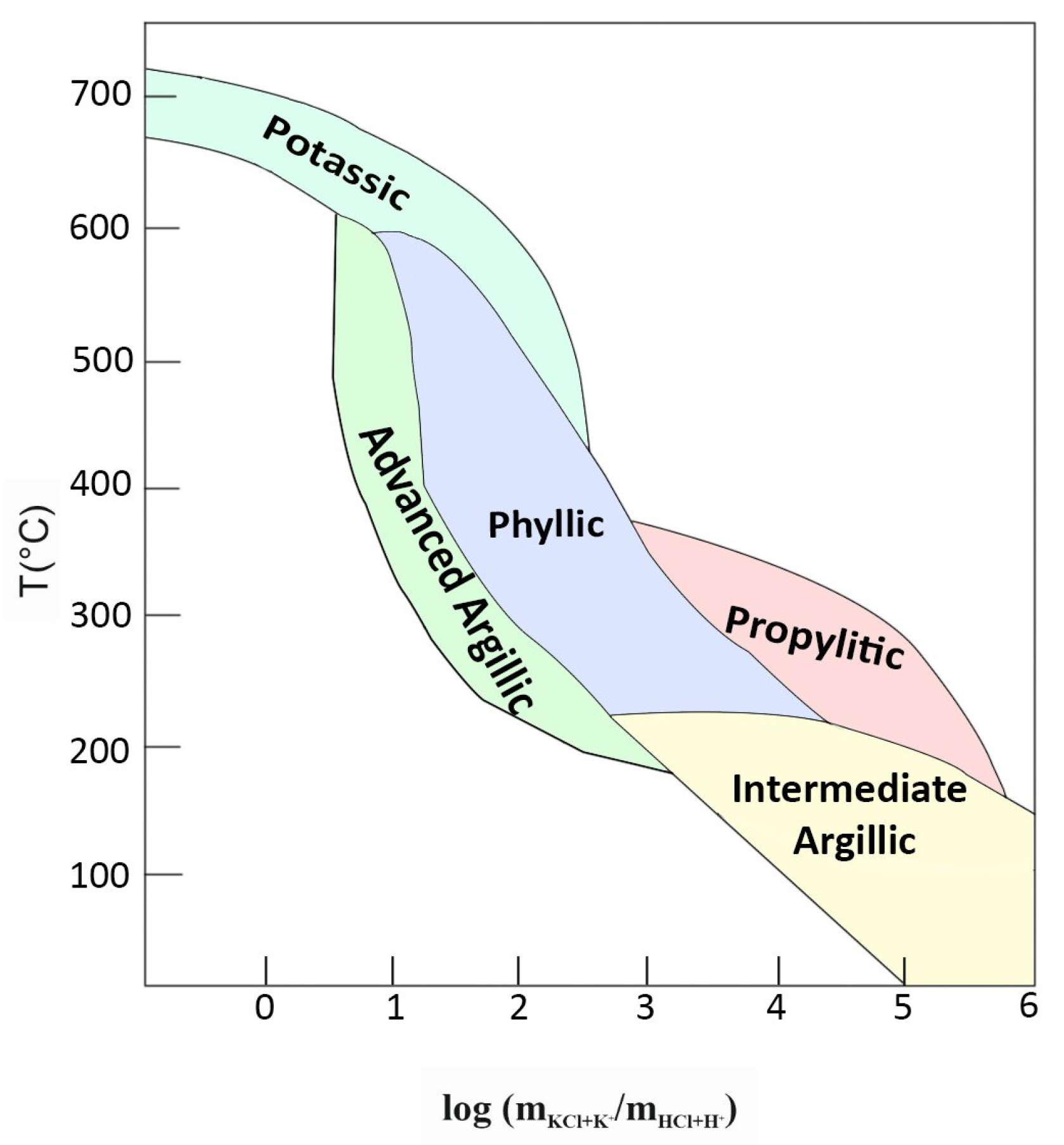
1.1. Wall-Rock Alteration

Around or alongside orebodies of hydrothermal origin, host rocks (wall-rocks) are variably altered, in terms of color, texture, mineralogy, and bulk chemistry, by the activity of these hot solutions. Variations are usually present from the ore zone outwards. Such spatial changes generally have a close temporal relationship with ore deposition. The most useful explorational and scientific aspects of hydrothermal alteration is their zoning, defined as “the spatial distribution patterns of major or trace elements, mineral species, mineral assemblages, or textures” [3], and is related to rock types, mineralogy, physical rock discontinuities (structures), and intensity (type) of alteration. Hydrothermal fluids chemically attack the mineral constituents of wall-rocks, forming secondary mineral assemblages in equilibrium with evolving physicochemical conditions [4].

In the entire spectrum of hydrothermal alteration, the most conspicuous zoning type is that of porphyry Cu (±Au, ±Mo) deposits in which alteration zones are arranged as concentric shells [5]. Porphyry deposits arguably represent the most economically important and fertile class of nonferrous metallic mineral resources. These deposits are characterized by sulfide and oxide ore minerals in veinlets and disseminations in large volumes of hydrothermally altered rock. Metals are transported as complex ions in the circulating hydrothermal fluids. As ${\mathrm{H}}^{+}$ metasomatism increases and temperature decreases, alteration types move from potassic to propylitic, phyllic, intermediate argillic, and advanced argillic, creating zones enriched in certain minerals, thereby allowing to focus exploration activity towards exact targets.

1.2. Conceptual Basis of the Research Problem

State-of-the-art techniques to typify and quantify wall-rock alterations include the application of mineralogical (for example, alteration indices that use normative minerals) and chemical (for example, mass balance calculations) approaches [6], which have their inherent disadvantages such as sensitivity to the composition of the precursors, difficulty of reconciling with mineralogical observations, and a component of subjectivity that invariably reduces the accuracy in the procedure of physical identification of alteration types. Furthermore, geochemical overprinting of an alteration type by subsequent phases of hydrothermal activity compounds to the problem of visual identification. In several settings, inaccurate or imprecise identification of alteration types has led to the dismissal of invaluable subsurface data, which subsequently proved misleading in the process of ore discovery.

Another pathway is to use supervised classification via machine learning (ML) based on geochemical analyses of drill cores. As mineralization is typically characterized by sampling less than 0.001% of the entire ore deposit, ML classification results in significant uncertainty compounded by high geological variability. These factors introduce unique risks to the profitable exploitation of mineral resources. The core challenge of mineral resource modeling lies in predicting the spatial distribution of rock types, wall-rock alteration types, and metal grades within the 3D subsurface of a deposit based on sparse drill core data collected at scattered locations.

1.3. Novel Contributions

Traditionally, the supervised classification of wall-rock alteration types has relied on whole-rock geochemical assays involving concentrations and transformed values of major oxides, alkali and alkaline-earth elements, and other chemical constituents—typically encompassing 55–60 feature variables. This study introduces a pioneering case for the classification of alteration types by just the concentrations of four metals and three metal sulfides, achieving a superior classification accuracy than in previous studies based solely on geochemical data of major elements. This contribution may be regarded as a novel discovery, primarily due to the general scarcity of publicly available proprietary drill hole data sets and, more specifically, the limited availability of laboratory data concerning the solubilities and thermodynamic stability conditions of metal sulfides relative to rock-forming silicates.

The proposed methodology extends the framework established by [7], who combined kriging with machine learning for rock type prediction. The present study introduces a key innovation by replacing kriging with geostatistical simulation, and by using nugget effect filtering to remove short-scale spatial variation (“noise”) in laboratory-measured values. Specifically, each original feature at a data location will be substituted with 50 normally distributed simulated proxies to improve predictive performance and to quantify prediction uncertainty. The methodology circumvents reliance on the original observations by generating multiple realizations by stochastic simulation, which preserves the statistical and spatial behavior of the feature variables, except for short-scale variations.

A major benefit of this approach lies in its robustness under data constraints—specifically, scenarios characterized by (a) substantial missing values among features, (b) a restricted number of influential features, and (c) sparse sampling. To compare the importances of the two sets of features—the original measured set versus the simulated proxies—we tested the individual classification performances by a machine learning algorithm, namely eXtreme Gradient Boosting (XGBoost). The categorical response is a total of six different wall-rock alteration types spatially distributed within the ore deposit. To address class imbalance, a cost-sensitive classification strategy is furthermore employed, informed by criteria rooted in thermodynamics and mineral exploration, to minimize the expected misclassification cost and to improve model reliability.

The principal research questions addressed in this scientific investigation are as follows:

1.

Is it possible to accurately classify wall-rock alteration types across any location within an ore deposit using concentrations of just four metals (Cu, Au, Mo, and As) and three metal sulfides (chalcopyrite, pyrite, and total sulfides), as input features derived from sampled data points? We posit that a classifier capable of discerning robust numerical patterns linked to distinct alteration types may achieve comparable or superior performance. The features employed are derived from a drill hole data set acquired under industry quality assurance and quality control standards. We will assess the accuracy of predictions by an evaluation with standard model performance metrics for classification.

2.

Does the implemented methodology provide an advantage with regards to its robustness under data constraints? Specifically, two distinct scenarios are evaluated to assess model performance under data constraining conditions: (i) substantial missing values among feature variables, and (ii) sparse spatial sampling. In the first scenario, missing feature values are imputed using the median value computed per alteration type for each corresponding input feature variable. In the second scenario, records with incomplete feature sets are excluded, and only isotopically sampled data points are retained to ensure reliability in spatial representation. The predictive performance for each scenario is evaluated using standard metrics, including accuracy, precision, recall, and F1-score. Comparative analysis of these results will inform the methodology’s resilience and applicability in real-world geochemical classification tasks.

3.

In the presence of unbalanced data—where certain wall-rock alteration types are overrepresented while others are sparsely sampled—does a cost-sensitive classification strategy yield superior predictive accuracy? Two methodological approaches are evaluated: (i) classification of the proxy data set with integration of XGBoost with a cost-matrix informed by thermodynamic and mineral exploration criteria to minimize expected misclassification cost, and (ii) classification of the proxy data set without integration of XGBoost with a cost-matrix. Model performance is assessed using standard metrics (accuracy, precision, recall, and F1-score), thereby providing a robust basis for evaluating the effectiveness of cost-sensitive learning under class imbalance.

The objective of this paper is to develop a hybrid approach combining geostatistical simulation and machine learning, called Geostatistically Enhanced Learning, which aims (1) to classify wall-rock alteration types at any location within an ore deposit using assay grades of metals (Cu, Au, Mo, and As) and metal sulfides (chalcopyrite, pyrite, and total sulfides) as input features with short-scale spatial variations, measurement errors, and missing information, and (2) to quantify the uncertainty associated with the predictions.

The outline is as follows: Section 2 gives a general description of related work and their limitations. Section 3 provides a theoretical background to the working principle of supervised classification with XGBoost and geostatistical simulation, as adopted in this research. The proposed methodology is then introduced in Section 4. Section 5 presents the data set of the case study and the results of the classification problem. Section 6 provides a discussion of the advantages of our proposal and its practical implications. Section 7 concludes the paper, while details on the experimental setup and parameter fitting are provided in Appendix A and Appendix B.

2. Related Work & Limitations

At first glance, the scientific problem in this investigation does not necessitate merging machine learning (ML) algorithms with those of geostatistics: the problem is simply one of classifying the likely alteration type associated with a given pattern of grade variations measured on drill cores, for which ML can be applied directly. For an overview of ML algorithms and their applications to alteration mapping and, more generally, to mineral exploration and mineral prospectivity mapping, see [8,9,10,11,12,13,14,15,16,17,18,19,20,21] and the references therein.

Yet, there are additional dimensions to the problem, making it substantially more complex. In particular, the following should be considered:

1.

Elemental and mineralogical concentrations (grades) are regionalized variables that exhibit spatial auto- and cross-correlations. In other words, the concentrations measured at a drill core bring information on the concentrations at surrounding locations, therefore, indirectly on the alteration class at these locations. Ignoring the information of neighboring drill cores, therefore, implies a loss in efficiency of ML classifiers.

2.

The dependence relationships between alteration classes and elemental and mineralogical concentrations furthermore depend on the spatial scale. While geochemical assays often exhibit short-scale variability and isolated occurrences of outlying values, the same does not happen with the prevailing alteration classes, the variations in which are more regular in space. Accordingly, ML classifiers would perform better if they were able to “extract” from the elemental and mineralogical concentrations the information that relates to the same spatial scale as the alteration classes, i.e., without short-scale variability.

3.

Measurement errors affect the quality of drill core data. It is well-known [22] that geochemical analyses are subject to errors arising from the sampling, preparation, and assaying of drill cores. In the geostatistical modeling of drill core data, these errors are one source of the well-known nugget effect in covariance functions and variograms [23], while in ML classification, they entail a loss in efficiency compared to what would be obtained by training the classifier on error-free data.

4.

Grade data sets are often heterotopic; that is, not all the grade variables are sampled at all the drill cores, which translates into missing values of different elemental and mineralogical grades. The traditional method for handling missing values in a data set is to impute with realistic values. Then arises the question: which value is realistic and which is not?

All the previous points originate from the fact that the classification problem at hand is not only of statistical nature, but also of spatial nature due to the spatial dependence of the feature and response variables and their spatial sampling design, and advocate for a spatial statistical (geostatistical) treatment of these variables.

Although traditional ML approaches were not developed for modeling spatial stochastic processes because of their inherent inability to account for the nature of spatial dependency (the spatial correlation structure) intrinsic to such processes, attempts have been made in the past decades for spatial prediction (either classification or regression) using alternate models or even integrating machine learning with geostatistical algorithms. Notable are that of spatial linear mixed-models [24], Convolutional Neural Networks [25,26], ML-Euclidean distance fields [27], ML-Residual Kriging [28,29,30,31,32,33], RF-GLS [34], RFsp [35], geographical RF [36,37], RF-Spatial Interpolation [38], spatial RF [39], and Kriging prior Regression [33]. Instead of fusing ML and spatial prediction algorithms, an alternative is to fuse the individual outputs of each by means of a weighting function, which allows an exact prediction at sampling locations [40,41]. ML models trained on sampling data can furthermore be applied on data obtained by geostatistical simulation in order to provide a measure of the uncertainty on the true unknown classes at unobserved locations [42,43,44].

However, the aforementioned proposals only address the problem of spatial correlations and, in some cases, the problem of heterotopic sampling designs, but not the other problems related to the spatial scale and the presence of measurement errors. Accordingly, to date, no comprehensive methodology has been proposed for regionalized classification problems, providing predictions at unobserved locations and uncertainty measures on these predictions, based on spatially correlated data carrying only partial information, mixing spatial scales, and affected by measurement errors.

In this respect, our proposal will address all the four aforementioned points. The key idea is to approach the missing data problem by training the ML classifier on proxy values generated by geostatistical simulation; in turn, these simulated values are “denoised”, i.e., they filter out the measurement errors and natural microvariability to only retain the spatial information adapted to the scale of variation in the response variable.

3. Theoretical Background

This section gives an overview of the tools and methods on which our proposal is built.

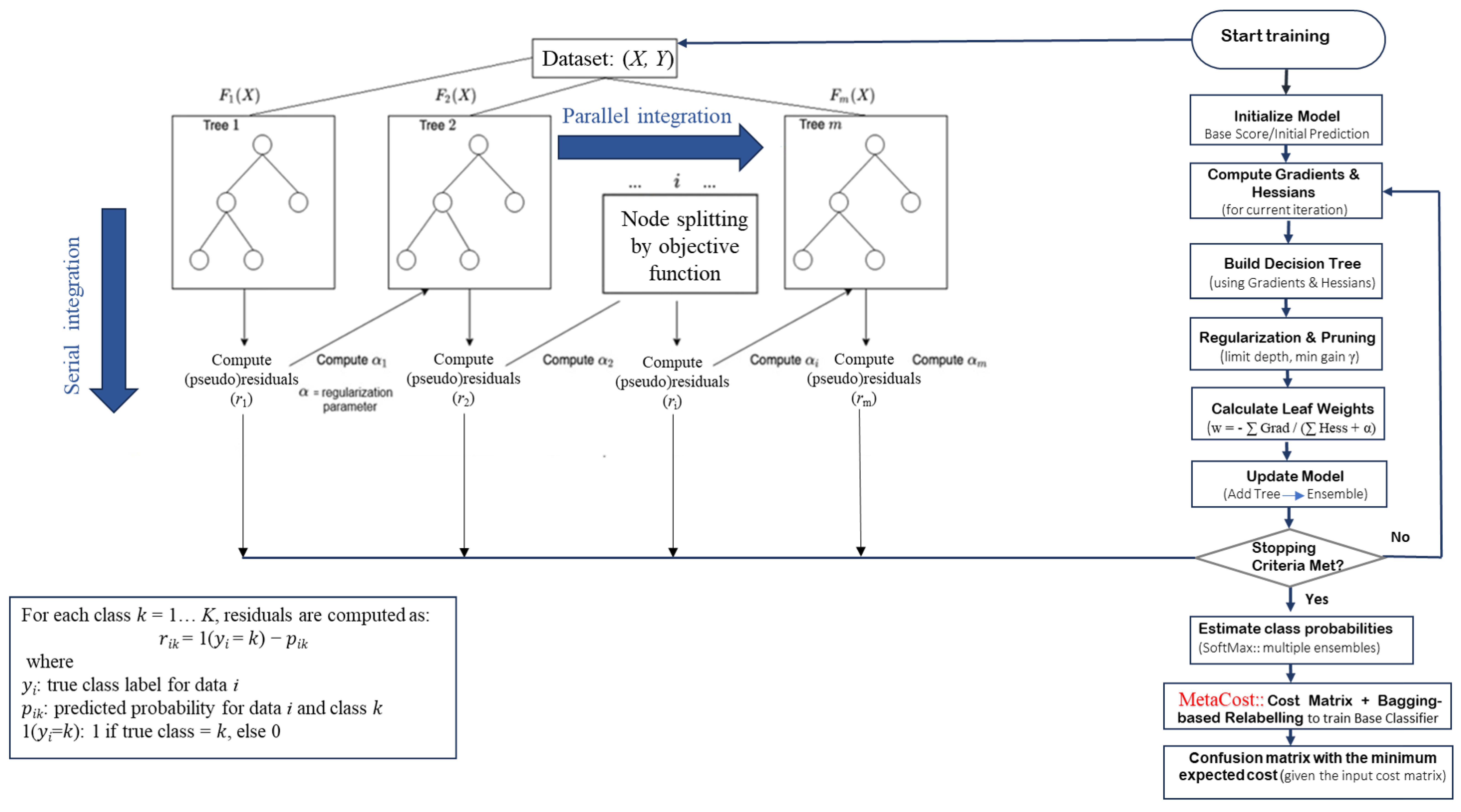
3.1. Basics on XGBoost Classification

XGBoost, short for eXtreme Gradient Boosting [45], an optimized implementation of gradient boosting [46], is a tree-based ensemble learning method. This ensemble is created by training a weak model and then training another model to correct the residuals or mistakes of the model before it. It has built-in parallel processing to train models on large data sets quickly. XGBoost also supports customizations allowing users to adjust model parameters to optimize performance based on the specific problem.

How does XGBoost work? It builds decision trees sequentially, with each tree attempting to correct the mistakes made by the previous one. The process can be broken down as follows:

1.

Start with a base learner: The first model decision tree is trained on the data.

2.

Calculate the errors: After training, the first tree the errors between the predicted and actual values are calculated.

3.

Train the next tree: The next tree is trained on the errors of the previous tree. This step attempts to correct the errors made by the first tree.

4.

Repeat the process: This process continues with each new tree trying to correct the errors of the previous trees until a stopping criterion is met.

5.

Combine the predictions: The final prediction is a combination of the predictions from all the trees.

XGBoost minimizes a regularized objective function given by [45]

$$\mathcal{L}=\sum _{i=1}^n\ell (y_i,{\widehat{y}}_i)+\sum _{j=1}^m{\mathrm{\Omega }}_j,$$

(1)

where ℓ is a differentiable convex loss function that measures the difference between the prediction ${\widehat{y}}_i$ and the target $y_i$ for each training data (with index i ranging from 1 to n), whereas the term ${\mathrm{\Omega }}_j$ is a mapping that depends on the number of leaves in the j-th tree (with index j ranging from 1 to m) and the output for each leaf node. The sum of ${\mathrm{\Omega }}_1,\dots ,{\mathrm{\Omega }}_m$, known as the regularization parameter, penalizes the complexity of the model, i.e., the set of regression tree functions, and helps to smooth the final learnt weights to avoid overfitting. Intuitively, the regularized objective will tend to select a model employing simple and predictive functions. When the regularization parameter is set to zero, XGBoost falls back to the traditional gradient tree boosting.

The workflow in Figure 1 enables XGBoost to build a robust classifier by sequentially adding trees that correct the errors of the previous ones, optimizing the model’s performance through gradient boosting and regularization techniques. The implementation details are provided next.

3.1.1. Step 1: Data Input and Preprocessing

1.

Input Data: Provide the feature matrix and corresponding target labels.

2.

Preprocessing:

• Encode categorical variables (for example, one-hot encoding).
• Normalize or standardize features if necessary.
• Split the data set into training and test sets.

3.1.2. Step 2: Model Initialization

1.

Initial Prediction: Set an initial prediction for all instances. For classification, this is often the log odds of the positive class.

2.

Parameter Setup: Define hyperparameters such as learning rate, maximum tree depth, and regularization terms. A Bayesian optimization scheme (Optuna) is implemented for hyperparameter tuning.

3.1.3. Step 3: Iterative Boosting Process

For each boosting round, the following steps are performed:

1.

Compute Gradients and Hessians: Calculate the gradient (first derivative) and Hessian (second derivative) of the loss function with respect to the current predictions.

2.

Construct a Decision Tree:

• Use the computed gradients and Hessians to build a decision tree that predicts the residuals.
• Determine the best splits by maximizing the gain, which measures the improvement in the loss function.
• Update the model’s predictions by incorporating the scaled output of the newly constructed tree.

3.1.4. Step 4: Objective Function Optimization

1.

Loss Function: XGBoost minimizes a regularized loss function (Equation (1)) that combines the training loss (for example, logistic loss) and a regularization term to penalize model complexity.

2.

Regularization: Helps prevent overfitting by controlling the complexity of the model.

3.1.5. Step 5: Output Aggregation and Prediction

1.

Aggregate Outputs: Sum the outputs from all trees to obtain the final prediction scores.

2.

Apply Softmax Function: Convert the aggregated scores into probabilities for each class using the softmax function.

3.

Final Prediction: Assign the class label with the highest probability as the predicted class.

3.1.6. Step 6: Model Evaluation

1.

Performance Metrics: Evaluate the model using appropriate metrics such as accuracy, precision, recall, F1-score, and confusion matrix.

2.

Cross-Validation: Optionally, perform cross-validation to assess the model’s generalization ability.

3.2. Basics on MetaCost

MetaCost [47] is a method used to make classifiers cost-sensitive by minimizing the expected cost of misclassification. Here is a high-level overview of how it works:

1.

Training Multiple Classifiers: MetaCost works by training multiple base classifiers on various bootstrap samples (random samples with replacement) of the original training data set.

2.

Estimating Class Probabilities: For each instance in the training set, MetaCost uses the trained classifiers to estimate the probabilities of it belonging to each possible class.

3.

Cost-Sensitive Reclassification: MetaCost then reclassifies each instance based on these estimated probabilities and a given cost matrix. The cost matrix defines the cost associated with each type of misclassification (for example, the cost of predicting Class A when the true class is Class B).

4.

Final Classifier: Finally, MetaCost trains a single classifier on the reclassified data, producing a cost-sensitive classifier that minimizes the expected misclassification cost.

The key points are the following:

• Bootstrap Sampling: This technique creates multiple random samples from the original training set to improve the robustness of the classifier.
• Cost Matrix: The cost matrix is crucial as it defines the costs associated with different types of misclassifications, guiding the reclassification process.
• Meta-Learning: MetaCost is considered a meta-learning algorithm because it builds upon other classifiers, transforming their predictions into cost-sensitive ones. MetaCost is effective in scenarios where misclassification costs vary significantly. It helps make more informed decisions by taking the costs into account rather than just aiming for the highest accuracy.

3.3. Tuning the XGBoost Classifier

Bayesian optimization using Optuna is an efficient method for hyperparameter tuning that models the objective function as a probabilistic surrogate (usually a Gaussian Process or Tree-structured Parzen Estimator). Instead of blindly searching the parameter space like grid or random search, it uses past evaluation results to intelligently choose the next set of hyperparameters to test. Optuna automates this process and is highly flexible, supporting pruning of unpromising trials and GPU acceleration. In the given code, it is used to optimize an XGBoost classifier by maximizing the weighted F1-score across stratified cross-validation folds.

3.4. Uncertainty Analysis

The bootstrap resampling [48] part of the code focuses on generating an ensemble of XGBoost classifiers by repeatedly resampling the training data set with replacement. In the present study, for each of 50 bootstrap iterations, a new training subset is created, and an XGBoost model—using the previously optimized hyperparameters—is trained on this subset. Each model then makes predictions on the same test set (data with complete information of the feature variables), resulting in a distribution of 50 predicted classes for every test data. By analyzing these predictions, the most frequently occurring class is selected as the final output for each sample, and the proportion of models that voted for this class is calculated as a confidence score. This method captures the variability in the model’s predictions, offering a way to assess prediction stability and quantify the uncertainty in classification outcomes.

3.5. Basics on Geostatistical Simulation

Geostatistical simulation is aimed at constructing a set of regionalized variables that have the same statistical and spatial distributions as a set of original variables. Therefore, although they are fictitious, the simulated variables are realistic and behave like the true ones.

How does geostatistical simulation work?

The original regionalized variables are interpreted as realizations of spatial random fields, and the simulated variables are just other realizations of the same random fields [23]. Accordingly, one needs to (1) specify a random field model and (2) construct realizations of this model.

Concerning the first point, the most widespread model in the case of a quantitative regionalized variable is the multigaussian model, where the variable is seen as a monotonic transform of a standard Gaussian random field. The model only depends on the definition of a transformation function, which can be estimated by applying a quantile–quantile transformation of the data to a standard normal distribution, and of a covariance function for the Gaussian random field. In the multivariate setting, a Gaussian transformation must be defined for each variable and the covariance function becomes matrix-valued, that is, it contains direct covariance functions in its diagonal elements, which describe the auto-correlations of the Gaussian random fields, and cross-covariance functions in its off-diagonal elements, which describe their cross-correlations. In applications, direct and cross-variograms are often used in place of covariance functions. Covariances or variograms can be experimentally estimated from a set of data scattered in space, then modeled by theoretical functions. The reader is referred to [23,49] for technical details.

Concerning the second point, the construction of simulated realizations or “scenarios” requires the definition of an algorithm. In the case of the multigaussian model, numerous algorithms have been designed; see [23,50] for a comprehensive survey. An additional important aspect is the conditioning of the simulation, which enforces the simulated scenarios to reproduce the observed data values at the data locations. Such a conditioning can be realized by use of kriging (univariate setting) or cokriging (multivariate setting) to post-process the non-conditional realizations and convert them into conditional [23].

4. Geostatistically Enhanced Learning for Supervised Classification

Our proposal incorporates the following elements:

1.

Supervised classification: In supervised learning, the ML algorithm “learns” to recognize a pattern or make general predictions using known examples. Supervised learning algorithms create a map, or model, $\mathit{f}$ that relates a data (or feature) vector $\mathit{x}$ to a corresponding label or target vector $\mathit{y}$: $\mathit{y}=\mathit{f}\left(\mathit{x}\right)$ using labeled training data—data for which both the input and corresponding label (${\mathit{x}}^{\left(i\right)},{\mathit{y}}^{\left(i\right)}$) are known and available to the algorithm—to optimize the model. A well-trained model should be able to generalize and make accurate predictions for previously unseen inputs.

2.

Extreme Gradient Boosting (XGBoost): It emerges as a top-choice classifier for its robustness against overfitting, minimal feature engineering, and ability to manage high-dimensional feature sets and sparse inputs [45]. Recent research shows that in terms of predictive accuracy, XGBoost generally has an advantage over single decision trees, often outperforms Random Forests by a margin in many cases, and is competitive with or better than Support Vector Machines and Neural Networks for tabular data sets [51,52].

3.

MetaCost: This algorithm is designed for cost-sensitive classification and minimizes the expected cost of misclassifications, rather than their number [47].

4.

Variogram analysis: It is the process of calculating experimental covariances or variograms that capture auto- and cross-correlations of spatial data and of fitting them with valid functions that are then inputted in geostatistical simulation [23].

5.

Conditional simulation: It generates multiple scenarios that reproduce the statistical and spatial behavior of one or more regionalized variables, and the observed values of these variables [23].

6.

Nugget effect filtering: The short-scale variations in a regionalized variable (nugget effect, reflecting measurement errors and natural microvariability) can be filtered out when delivering the simulated values [53,54].

Overall, our proposed Geostatistically Enhanced Learning for supervised classification consists of nine steps (Figure 2; details in the next subsections):

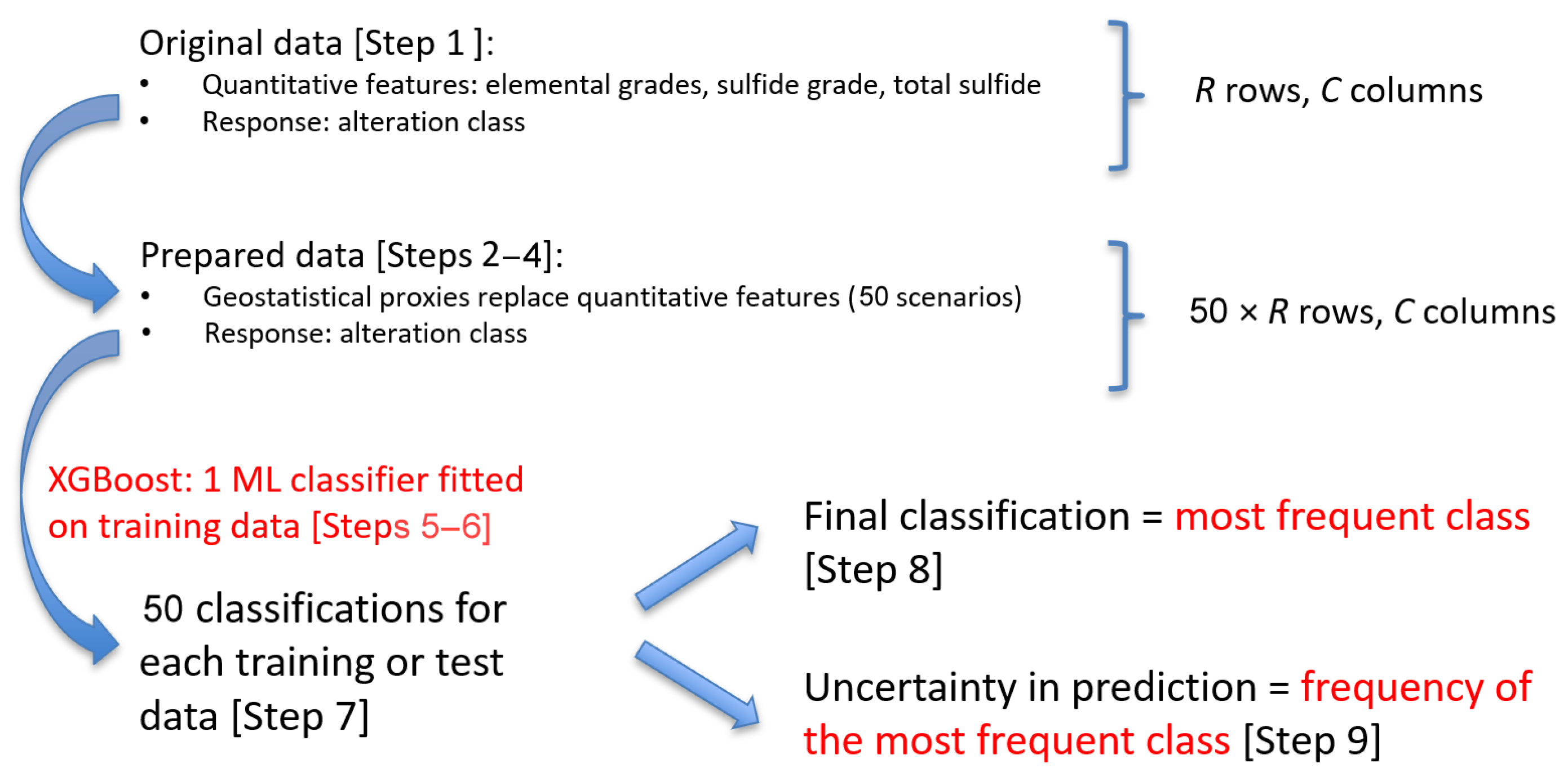
• Step 1: Data cleaning.
• Step 2: Transforming each feature variable to a normal scale.
• Step 3: Variogram analysis of the normal score transforms.
• Step 4: Geostatistical simulation with nugget effect filtering to replace the value of each original feature variable at each data location with 50 simulated proxies that are normally distributed.
• Step 5: Random splitting of the data set into training (70%) and test (30%) subsets.
• Step 6: Training XGBoost with MetaCost on the training data with the simulated proxies.
• Step 7: Applying XGBoost to obtain 50 classifications for each training or test data.
• Step 8: Selecting the most frequent classification at each data location.
• Step 9: Assessing the classification confidence at each data location by calculating the frequency of the most frequent class.

4.1. Geostatistical Simulation with Filtering to Create Proxy Variables (Step 4)

Provided with the direct and cross-covariances of the Gaussian-transformed feature variables, it becomes possible to simulate these variables at any location of interest. In this research, we used a continuous spectral algorithm, which relies on the Fourier transform of the covariance functions and on an importance sampling strategy [55]. The locations targeted for simulation are the training and test data locations.

The simulation can furthermore filter out the variability associated with any of the basic nested structures of the covariance model, in particular, the nugget effect that corresponds to natural microvariability and measurement errors. The general workflow for the simulation with nugget effect filtering is indicated in Figure 3. The formalism and equations can be found in [53].

The result of the simulation is a set of scenarios or realizations (50 in the present research). Each scenario provides a set of Gaussian random fields—the proxies—whose spatial correlation structure is given by the continuous component (without the nugget effect) of the covariance model, conditioned to the observed values of the feature variables of both the training and test data. Note that the response variable (alteration class) is not used in the constructions of the proxies.

An aspect worth emphasizing is the organization of the simulation results for their subsequent use in supervised classification. Unlike [53,54] who repeat the classification task on each simulated scenario, leading to as many classifiers as there are scenarios (50 in the present case), in this research we applied the classification only once, by considering a data set with an augmented number of rows (50 times more rows than the original data set) instead of an augmented number of columns (same number of rows as the original data set and 50 times more columns).

The benefit of this stratagem is threefold:

1.

The classifier needs to be trained only once.

2.

All the simulated scenarios are equally important in the classification process.

3.

This classifier can be applied to any set of simulated scenarios, even if they are not the same as the scenarios used to train the classifier. In other words, the simulated scenarios that have been used to train the classifier do not need to be extended to new locations where drill hole data become available, and the classifier does not need to be retrained.

4.2. Uncertainty Analysis Based on Simulated Proxies (Step 9)

Instead of 50 bootstrapped samples as proposed in Section 3.4, uncertainty analysis can be performed directly on the 50 sets of simulated proxies at the data locations. Specifically, the proxies at the training data are used to train a single XGBoost classifier, which is applied to the 50 sets of proxies at the test data locations. By analyzing the 50 predictions at each test data location, the most frequently occurring class is selected as the final output and the proportion of classifications matching this class is calculated as a confidence score.

5. Application Case Study

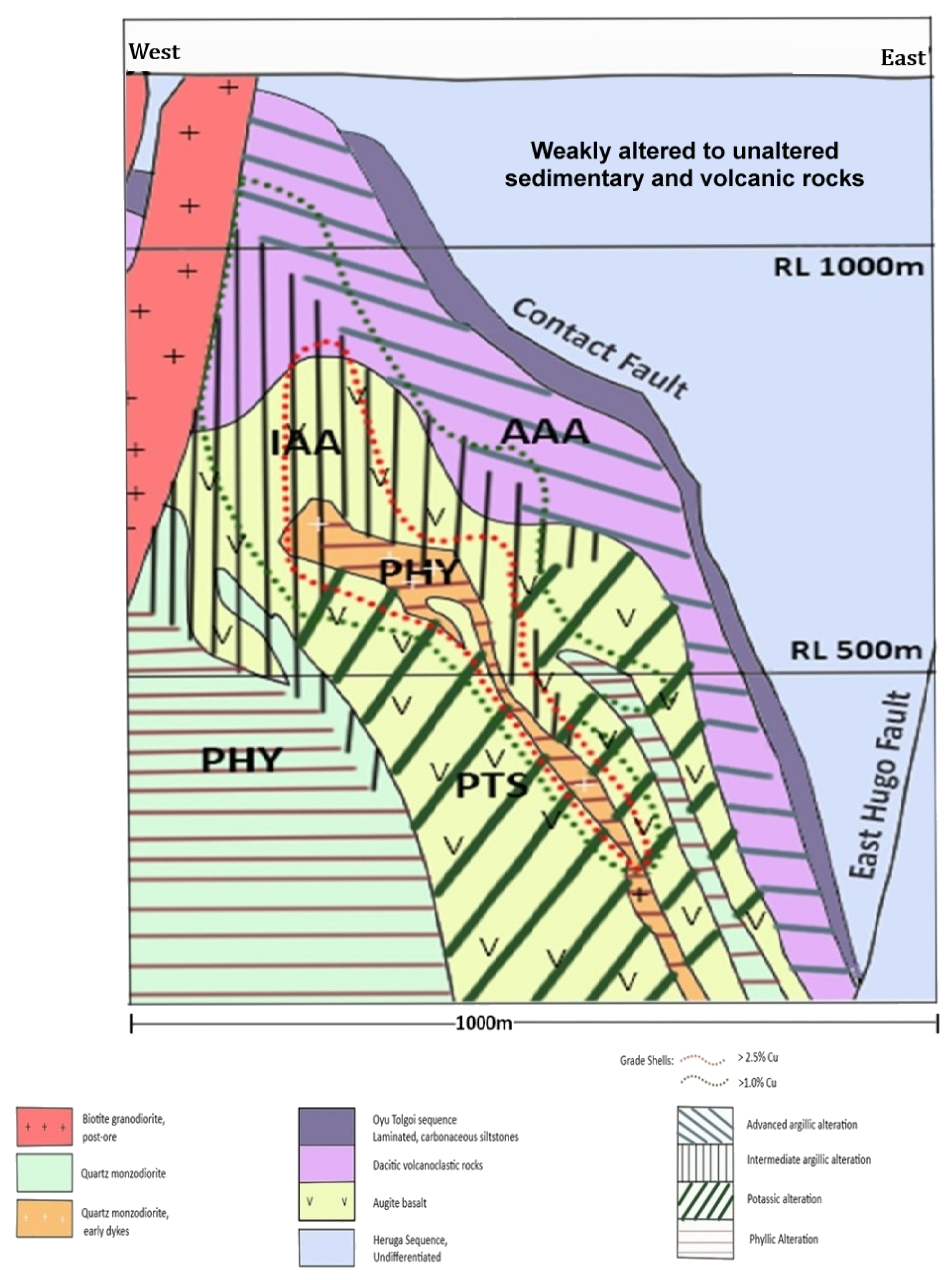
5.1. Deposit Geology

A chain of porphyry mineralization occurs within the Central Asian Orogenic Belt, extending for 5000 km from the Urals in the west to the Pacific coast in the east. The most prolific geologic period of ore formation, including the largest deposits, was during the Late Devonian and Early Carboniferous [56]. The mineralization process is characterized by intrusions of large volumes of granitic magma accompanied by the availability of metal-rich hydrothermal fluids, with ore localization controlled by structural features, rock types, and wall-rock alteration types. The details of the ore-forming process can be found in [57,58].

In Mongolia, porphyry mineralization occurs in two places: Erdenet and Oyu Tolgoi. Erdenet is located in Central Mongolia, whereas Oyu Tolgoi (43.0253° N, 106.8665° E) is located within the South Gobi Desert, about 650 km due south of the capital, Ulaanbaatar.

The latter constitutes a cluster of seven porphyry Cu-Au-(±Mo, ±Ag) deposits, the largest high-grade group of Palaeozoic porphyry deposits known in the world. The rock sequence surrounding this cluster of deposits is predominantly composed of basaltic to intermediate volcanic rocks of Devonian age, overlain by layered dacitic pyroclastic and sedimentary rocks intruded by basaltic and dolerite sills. The southern deposits (Southwest, Heruga North, and Heruga) are characterized by high Au (g/t)/Cu (%) ratios (0.8–3:1), whereas the Hugo Dummett (North and South) deposits are characterized by lower ratios (0.1–1:1) and hosted mainly by volcanic and plutonic rocks with extensive phyllic and advanced argillic hydrothermal alteration. The detailed geology and mineral exploration history in the Oyu Tolgoi district can be found in [59] and the references within. A simplified geological map of the area comprising the twin Hugo Dummett deposits can be found in [7].

The deposit concerned in this study is the Hugo Dummett South deposit, a polymetallic porphyry with economic grades of Cu, Au, and Mo (±Ag) and potentially deleterious grades of As, F, S, and Fe. It is hosted by an east-dipping basalt rock sequence intruded by porphyritic quartz-monzodiorite plutons. The deposit is both disrupted by, and bounded by fault displacements in four directional orientations. The mineralization occurs in an anastomosing network of stockwork veinlets of sulfides ± quartz and is associated with Late Devonian intermediate-to-high-K, porphyritic quartz-monzodiorite, emplaced as structurally controlled dykes and small plugs, followed by Late Devonian, post-mineral, biotite granodiorite intrusions. The Cu-Au mineralization at this deposit is centered on a high-grade copper (typically > 2.5%) and gold (0.5–2 g/t) zone of intense quartz stockwork veining. The stockwork is mainly localized within the quartz-monzodiorite intrusive; however, it also extends into the basaltic wall-rock units.

Table 1. Rock types observed in drill cores of the Hugo Dummett South deposit.

Serial Number	Rock Type	Age
1	Quaternary cover	Quaternary
2	Cretaceous clay	Cretaceous
3	Carboniferous andesite dykes	Carboniferous
4	Basalt dykes	Carboniferous
5	Carboniferous intrusive	Carboniferous
6	Carboniferous rhyolite dykes	Carboniferous
7	Faulted rocks	Late Devonian and older
8	Biotite granodiorite dykes	Late Devonian and older
9	Hydrothermal breccia	Late Devonian and older
10	Quartz monzodiorite	Late Devonian and older
11	Ignimbrite	Late Devonian and older
12	Augite basalt	Late Devonian and older
13	Hanging wall sequence	Late Devonian and older

shows the rock types encountered in drill holes within the Hugo Dummett South deposit along with their corresponding ages.

There are potentially multiple overlapping mineralizing phases. Hydrothermal alteration exhibits a strong lithologic control with a number of assemblages including a minor preserved potassic (PTS) suite, overwhelmed by the prominent, overprinting phyllic (PHY), advanced argillic (AAA), and intermediate argillic (IAA) alteration styles (Figure 4). Propylitic alteration (PRO) occurs as a weak outermost zone and has no associated mineralization.

5.2. Data Description

The data set under consideration comprised geological, geochemical, and survey information of 360 drill holes, with assays of thirteen chemical elements (Cu, Au, Ag, Mo, As, Fe, S, C, F, Pb, Zn, Cd, and Hg), mineral percentages, and alteration types. Drill core samples were composited to a length of 2.0 m. The training and test sets contained 18,758 and 8042 data, respectively, of which only 16,447 and 7068 have no missing value.

For classification purposes, 7 feature variables were selected, consisting of the concentrations of 4 chemical assays (Cu, Au, Mo, and As), 2 sulfide concentrations (chalcopyrite and pyrite), and total sulfide concentration (TS) that accounts for bornite, chalcopyrite, chalcocite, covellite, enargite, pyrite, pyrrhotite, molybdenite, galena, and sphalerite. Statistics on these variables are given in

Table 2. Statistics on target variable (alteration class) in the data table.

	Alteration Class	Alteration Code	Number of Records in Training Set	Number of Records in Test Set
Entire drill hole data base	Advanced argillic	AAA	5348	2377
	Intermediate argillic	IAA	2979	1383
	Phyllic	PHY	6478	2738
	Propylitic	PRO	2882	1131
	Potassic	PTS	475	230
	Unaltered	UAL	596	183
	All classes		18,758	8042
Drill hole composites without missing data	Advanced argillic	AAA	4427	2044
	Intermediate argillic	IAA	2883	1333
	Phyllic	PHY	5785	2426
	Propylitic	PRO	2650	1014
	Potassic	PTS	239	125
	Unaltered	UAL	463	126
	All classes		16,447	7068

and

Table 3. Statistics on feature variables in the data table (23,515 data points have information of all the features, of which 16,447 belong to the training set and 7068 to the test set).

Feature	Number of Records in Training Set	Number of Records in Test Set	Min.	Max.	Mean	St. Dev.
Cu (%)	16,811	7246	0.0	21.5	0.807	0.845
Au (ppm)	16,810	7246	0.0	26.8	0.097	0.285
Mo (ppm)	16,751	7218	0.06	3730	58.06	82.43
As (ppm)	16,448	7068	0.5	13,400	167.56	392.64
chalcopyrite (%)	18,758	8042	0.0	11.2	1.102	1.051
pyrite (%)	18,758	8042	0.0	38.0	2.011	1.970
TS (%)	18,758	8042	0.0	60.0	3.457	2.160

.

5.3. Geostatistical Modeling and Simulation of Proxies

The traditional multigaussian modeling workflow [23] was applied:

1.

Normal score transformation: The values of each of the 7 feature variables were converted into Gaussian values based on a quantile-quantile transformation of their experimental distribution into a standard Gaussian distribution. As a result, we obtained 7 Gaussian variables, which were used in the subsequent steps in place of the original feature variables.

2.

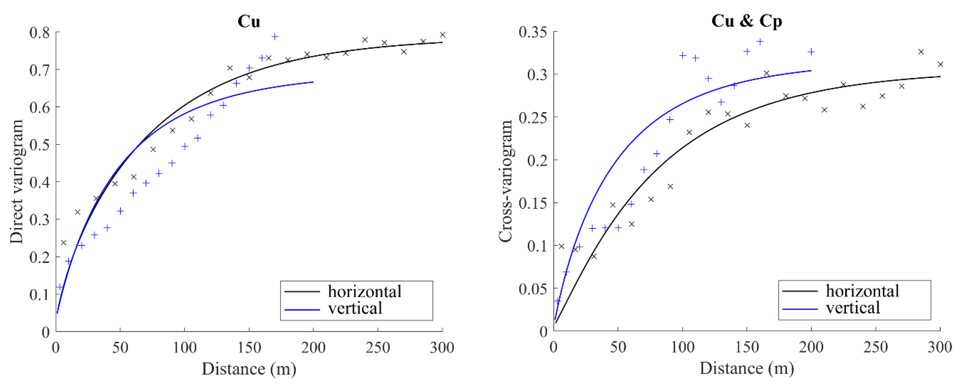
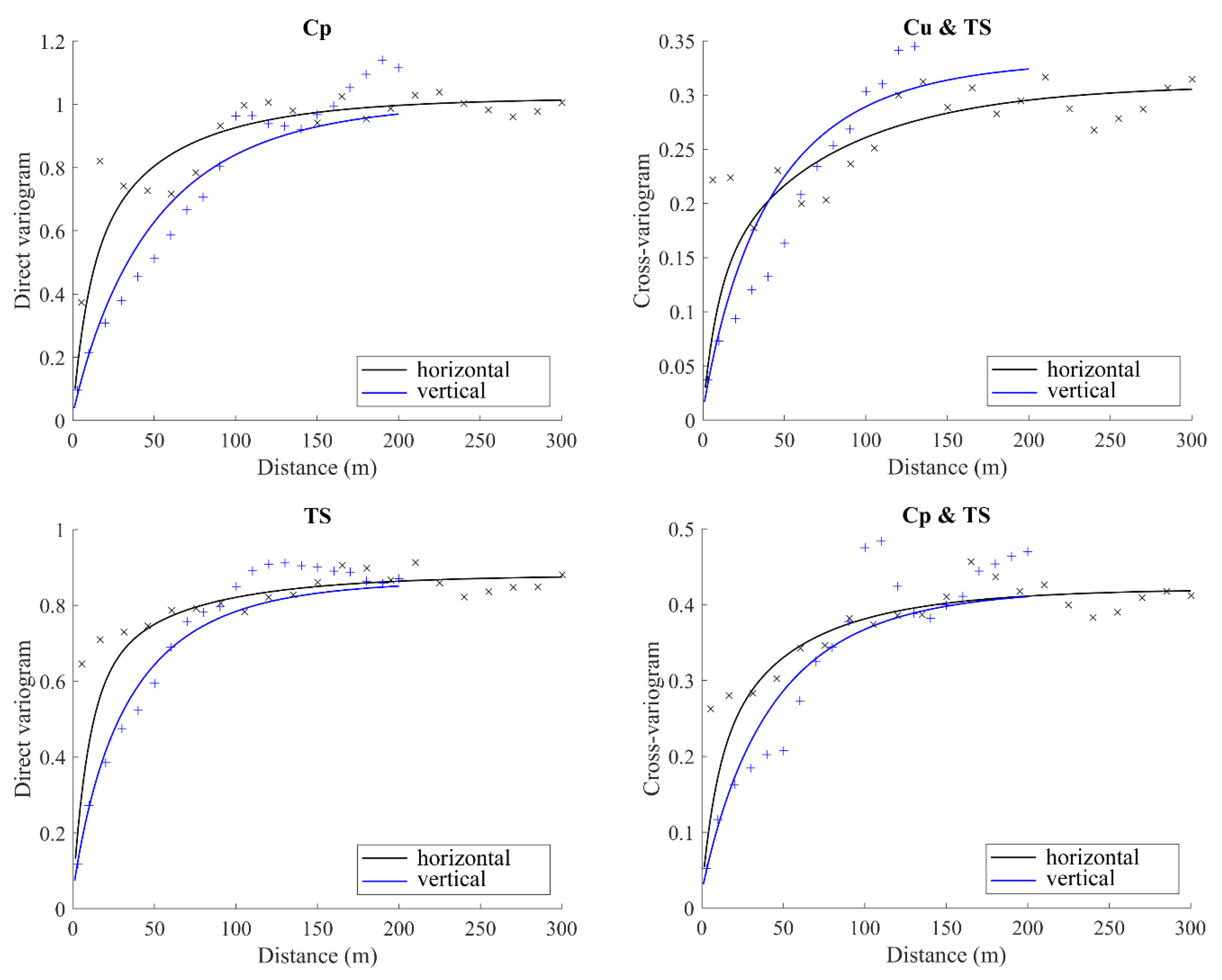
Variogram analysis: The experimental direct and cross-variograms of the normal score data were calculated along the horizontal and vertical directions, recognized as the main anisotropy directions, and fitted with a linear model of coregionalization [49] consisting of a nugget effect and nested exponential variograms with practical ranges between 25 m and 250 m (Figure 5). The fitting was performed with a semi-automated algorithm [60] that ensures the positive semidefiniteness of each coregionalization matrix of size $7\times 7$.

3.

Simulation of the proxies at the data locations: A spectral algorithm was used to jointly simulate the 7 Gaussian variables at the data locations without the nugget effect component [53,55], and to condition the simulation to the normal score values observed at the 30 nearest data locations (including the target data location). This resulted in 50 sets of normally distributed proxies at the data locations. The proxies simulated at the training data locations were used for training the XGBoost classifier, while the proxies simulated at the test data were used for assessing the performance of the fitted XGBoost classifier and for uncertainty quantification.

5.4. Cost Matrix Definition

The misclassification cost matrix (

Table 4. Misclassification cost matrix obtained by adding two partial cost matrices.

		Predicted Class
		PTS	PRO	PHY	IAA	AAA	UAL
True Class	PTS	0	5	7	9	8	12
	PRO	5	0	10	12	9	10
	PHY	7	10	0	4	7	16
	IAA	9	12	4	0	5	16
	AAA	8	9	7	5	0	12
	UAL	12	10	16	16	12	0

) is defined as the sum of two partial cost matrices (

Table 5. Partial cost matrix based on thermodynamic parameters.

		Predicted Class
		PTS	PRO	PHY	IAA	AAA	UAL
True Class	PTS	0	1	3	5	6	8
	PRO	1	0	2	4	5	8
	PHY	3	2	0	2	3	8
	IAA	5	4	2	0	1	8
	AAA	6	5	3	1	0	8
	UAL	8	8	8	8	8	0

and

Table 6. Partial cost matrix based on exploration criteria.

		Predicted Class
		PTS	PRO	PHY	IAA	AAA	UAL
True Class	PTS	0	4	4	4	2	4
	PRO	4	0	8	8	4	2
	PHY	4	8	0	2	4	8
	IAA	4	8	2	0	4	8
	AAA	2	4	4	4	0	4
	UAL	4	2	8	8	4	0

) scaled between 0 (no misclassification) and 8 (worst misclassification). The first partial cost matrix builds on thermodynamic parameters (temperature, activity of ${\mathrm{K}}^{+}$ and ${\mathrm{H}}^{+}$ ions, as shown in Figure 6, and pH), where the alteration types can be ordered as PTS, PRO, PHY, IAA, and AAA. The second partial cost matrix relies on exploration criteria and considers a trade-off between exploration drilling costs and missed opportunities for mineral discovery, where IAA and PHY are associated with a strong mineralization, AAA and PTS with a weak mineralization, and PRO and UAL (fresh rock) with no mineralization.

5.5. Experimental Setup

Two cases were examined, one based on the seven original feature variables, the other one based on simulated proxies with nugget-effect filtering instead of the original feature variables. In each case, the classifier was fitted on the training data subset and its performance is assessed on the test subset (Figure 7 and Figure 8).

1.

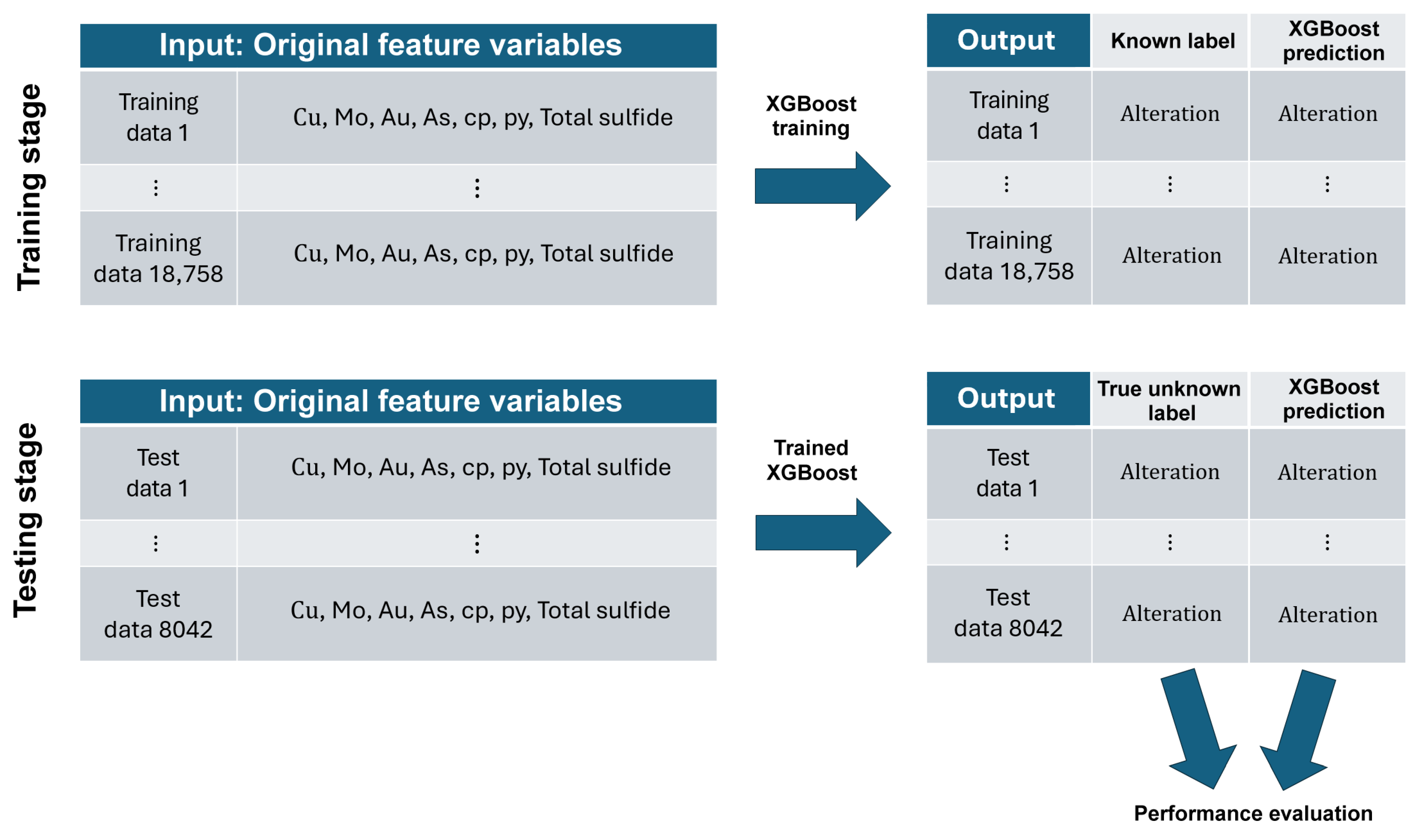
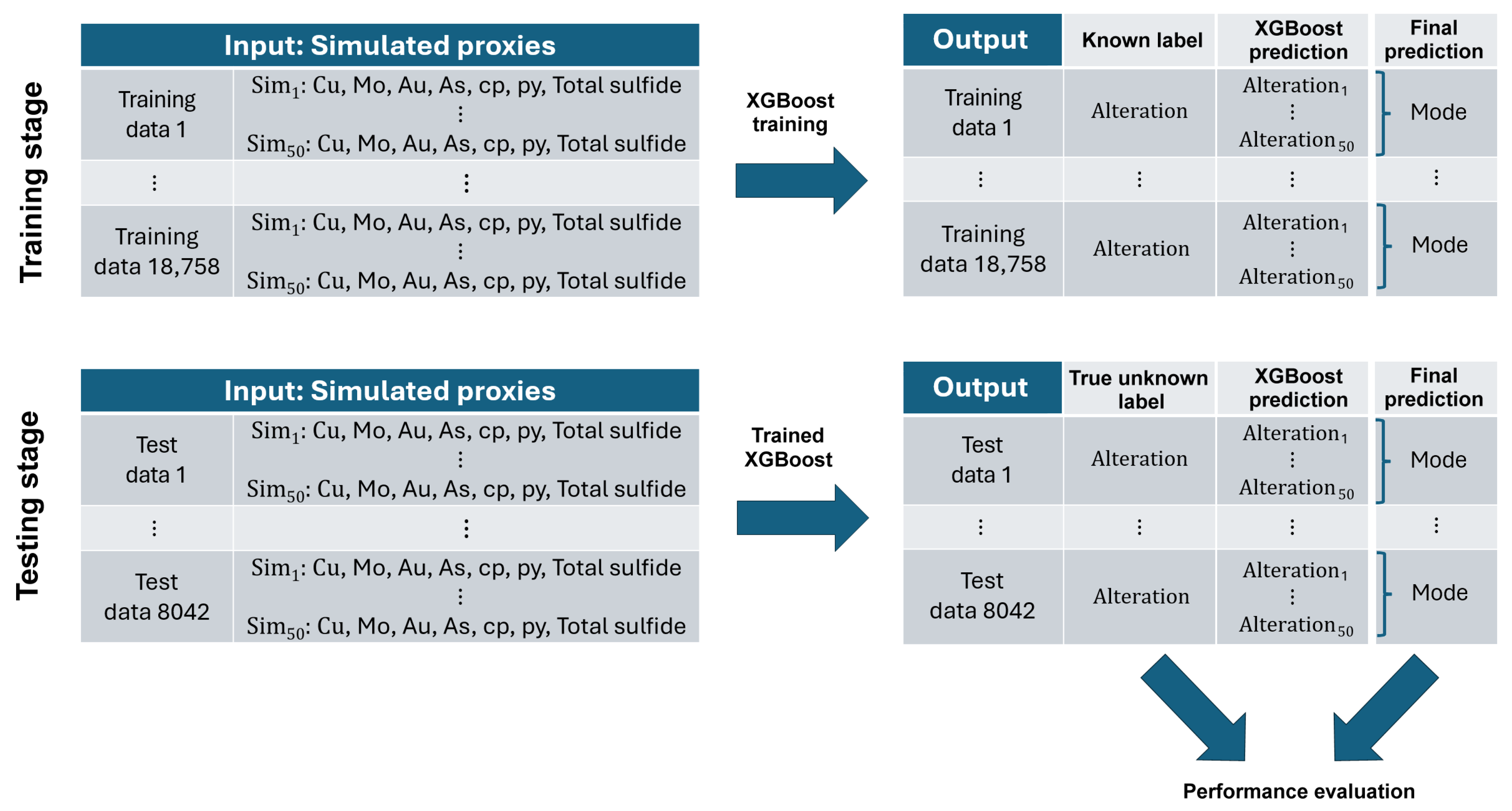
Experiment 1: This experiment was performed to answer the following question: does our implemented methodology provide an advantage with regards to its robustness under data constraints?

For case 1 (classification based on original feature variables), two distinct scenarios were evaluated to assess model performance under data constraining conditions: (A) substantial missing values among feature variables, and (B) sparse spatial sampling. In scenario A (Figure 7), missing feature values were imputed using the median value computed per alteration type, for each corresponding input feature variable. In scenario B, the training data with missing values were excluded, and only isotopically sampled data points were retained.

For case 2 (classification based on simulated proxies), data imputation or data remotion was not needed, insofar as conditional geostatistical simulation could be performed with heterotopic data (Figure 8).

2.

Experiment 2: This experiment was performed to answer the following question: in the presence of unbalanced data, does a cost-sensitive classification strategy yield superior predictive scores?

For case 2, two methodological scenarios were evaluated to answer the question: (A) classification of the proxy data set with integration of XGBoost with a cost-matrix informed by thermodynamic and mineral exploration criteria to minimize expected misclassification cost (same as case 2 of Experiment 1), and (B) classification of the proxy data set without integration of XGBoost with any cost-matrix.

All the analyses and workflows (Appendix A) in this study were implemented in Matlab (R2023b) and Python (v3.12) using custom-developed scripts. In detail, Matlab scripts were used for the geostatistical modeling and simulation, including normal score transformation of the feature data, calculation of direct and cross-variograms, semi-automated fitting of a linear model of coregionalization, and spectral simulation to generate the proxies. The outputs of this part of the workflow consisted of comma-separated values (CSV) files with the spatial coordinates, true alteration classes, and simulated proxies for the training and test data points.

Python scripts were used for training the XGBoost classifier and for the subsequent evaluation at the test data points. The scripts were written in Python 3.12 and rely on open-source libraries, including NumPy, Pandas, Scikit-learn, XGBoost, Optuna, Seaborn, prettycm and SciPy for data processing, model training, statistical computations, and data visualization. Data preparation and feature encoding were performed in Pandas, while XGBoost served as the core machine learning algorithm within the MetaCost framework to incorporate misclassification costs during training. The simulated data set workflow employed scripts to train the classifier on the simulated proxies obtained with Matlab, subsequently computing modal (most frequent) class outcomes across 50 realizations, followed by performance evaluation using custom metric functions. The traditional dataset workflow implemented MetaCost directly on observed data for comparison. Additional scripts were developed for bootstrapping and frequency–accuracy analysis to assess prediction confidence.

All the data files and source codes for the Matlab and Python scripts are provided in public repositories, as indicated in the Data Availability Statement at the end of this paper.

5.6. Prediction Results

The classification scores on test data for the two experiments (Experiment 1 and Experiment 2) under consideration are provided in

Table 7. Classification scores on test data for Experiment 1 (A).

Metric	Classification from Original Feature Variables (8042 Test Data)	Classification from Geostatistical Proxies (8042 Test Data)
Accuracy	0.66	0.77
Cohen’s Kappa	0.55	0.69
Precision	0.67	0.77
Recall	0.66	0.77
F1-score	0.66	0.77
Specificity	0.92	0.95
Sensitivity	0.55	0.74

,

Table 8. Classification scores on test data for Experiment 1 (B).

Metric	Classification from Original Feature Variables (7068 Test Data)	Classification from Geostatistical Proxies (8042 Test Data)
Accuracy	0.69	0.77
Cohen’s Kappa	0.58	0.69
Precision	0.69	0.77
Recall	0.69	0.77
F1-score	0.69	0.77
Specificity	0.93	0.95
Sensitivity	0.68	0.74

and

Table 9. Classification scores on test data for Experiment 2.

Metric	(A) Classification from Geostatistical Proxies with MetaCost (8042 Test Data)	(B) Classification from Geostatistical Proxies Without MetaCost (8042 Test Data)
Accuracy	0.77	0.75
Cohen’s Kappa	0.69	0.67
Precision	0.77	0.75
Recall	0.77	0.75
F1-score	0.77	0.75
Specificity	0.95	0.94
Sensitivity	0.74	0.73

, while the respective confusion matrices are displayed in Figure 9. Details on the parameter fitting are left to Appendix B.

5.6.1. Experiment 1

(A)

Test for the scenario where original missing feature values are imputed using the median value computed per alteration type, for each corresponding input feature variable, vs. proxy-based classification where imputation is not required (Table 7; Figure 9a,c).

(B)

Test for the scenario where training data with missing values are excluded, and only isotopically sampled data points are retained, vs. proxy-based classification where data remotion is not required (Table 8; Figure 9b,c).

5.6.2. Experiment 2

Test for the scenario where the proxy-based classification is run with (A) XGBoost integrated with a cost-matrix informed by thermodynamic and mineral exploration criteria to minimize expected misclassification cost and (B) XGBoost is not integrated with any cost-matrix (Table 9; Figure 9c,d).

5.6.3. Analysis

The results call for the following comments:

1.

In the traditional workflow, data imputation deteriorates all the scores ($-2\%$ to $-3\%$ in accuracy, precision, recall, and F1-score) with respect to the case when the missing data are simply removed (Table 7 and Table 8). This is a warning against “blind” imputation procedures that ignore the spatial correlation structure of the data.

2.

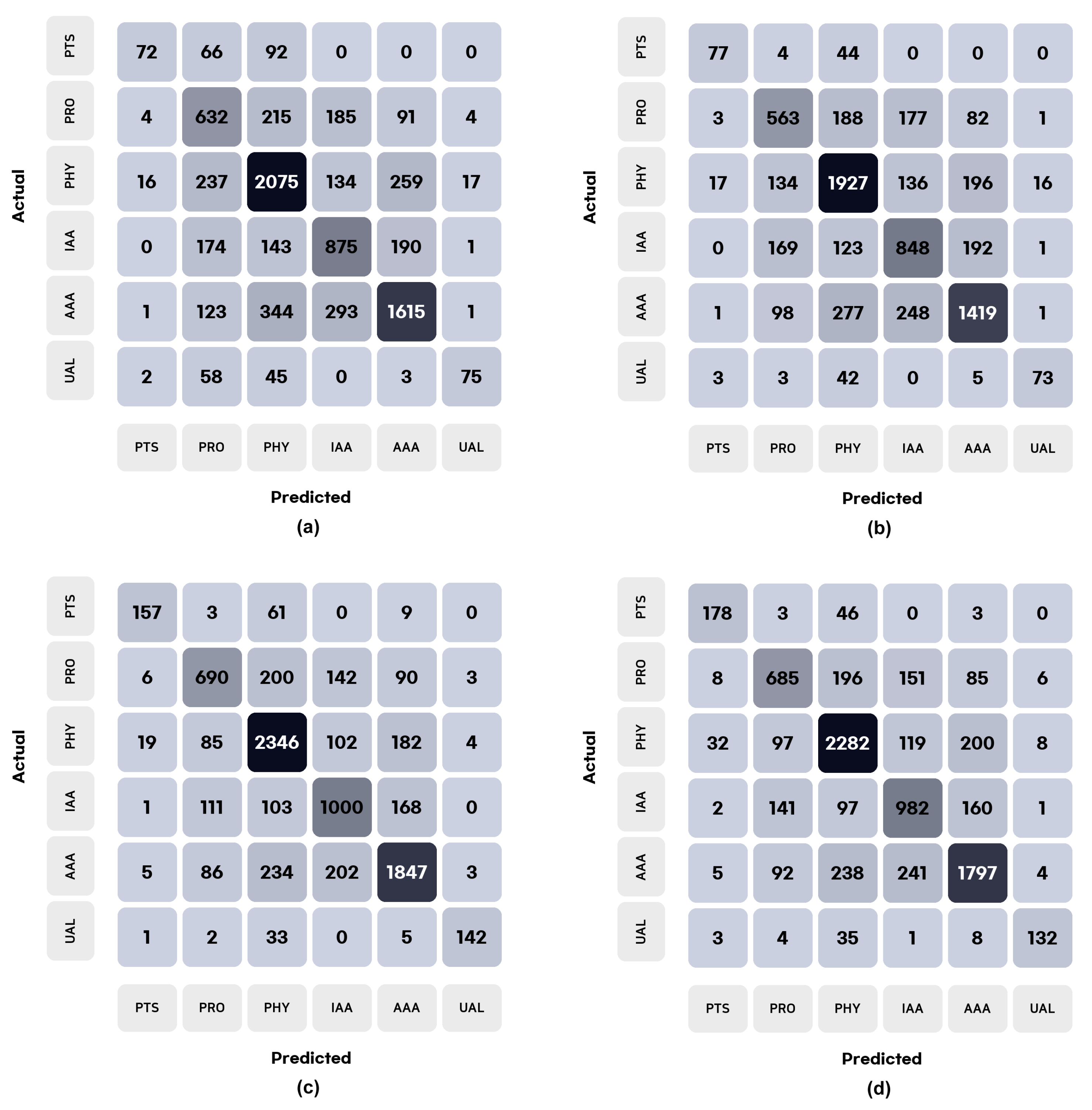
In all cases, the classification based on geostatistically enhanced learning outperforms the traditional workflow, with a significant improvement of all the scores ($+8\%$ to $+11\%$ in accuracy, precision, recall, and F1-score, when comparing cases 1 and 2 of Experiment 1; $+6\%$ to $+9\%$ when comparing case 1 of Experiment 1 and scenario B of Experiment 2). This indicates that geostatistically enhanced learning substantially reduces misclassifications, both false positives and false negatives, as corroborated by the confusion matrices in Figure 9.

3.

Although it is designed to minimize the expected cost of misclassifications rather than their number, MetaCost slightly improves the accuracy, precision, recall, and F1-score ($+2\%)$ when used in combination with the geostatistical proxies. This may be explained because the costs defined in Table 4 depend on regionalized properties of the alteration classes (thermodynamic and geology), therefore enhancing the classification with respect to costs that are blind to the spatial setting.

5.7. Prediction Uncertainty Quantification

Uncertainty quantification was performed on the most successful cases, corresponding to Experiment 1 (B) (Table 8).

In the first case, 50 classifiers were trained on as many training data sets obtained by bootstrap resampling and then applied to the test set, as explained in Section 3.4. The most frequent class was selected as the final output for each test data, and the proportion of classifiers that provided this class was calculated as a confidence score. In the second case, the confidence score at each test data location was also assessed by the frequency of the most frequent class in our methodology (Step 9; Section 4.2); for instance, a class obtained in 40 out of 50 scenarios should have an 80% probability of being the true one.

The confidence scores obtained in the first case turn out to considerably underestimate the true classification accuracy, while those obtained in the second case quantify much better the true classification accuracy (Figure 10).

6. Discussion: Significance and Outlook

This study combines two approaches that are traditionally separate: (1) geostatistical simulation to remove the noise affecting feature variables and to infill their missing values with proxies, and (2) an XGBoost classification to predict a categorical response from the simulated proxies. Such a workflow is a methodological leap beyond conventional practices where alterations are delineated by manual expert interpretation or by simpler (geo)statistical/ML methods [11,61]. Few works to date have so explicitly combined these techniques for 3D geological classification, making this case study methodologically noteworthy in the fields of exploration and mining geology.

6.1. Advantages of Using Simulated Proxies

The use of geostatistical simulation is multifold:

1.

Spatial context encoding: Geostatistical simulation injects knowledge of spatial continuity and geological trends into the data set. The proxies are not unconditionally simulated values—they honor the spatial locations, sample distributions, and variograms. Thus, when XGBoost trains on these features, it is indirectly learning from the spatial patterns of geochemistry and mineralogy, not just point values. This is a form of data augmentation that encodes the 3D spatial context, and constitutes a big advantage over using raw, point-sampled data where the spatial relationships would be invisible to the algorithm.

2.

Holistic use of data: Our method avoids discarding drill intervals that lack a particular measurement by filling in a geostatistically plausible value. Traditional ML models would either drop those samples or impute that feature value, losing information. Here, no part of the drill core data goes unused—every location has a full complement of features, albeit they are simulated. This means the ML classifier is not biased by only the complete-case data; it benefits from mineralogical indicators even where originally absent, because those gaps were filled in a geologically informed manner. The result is a classifier that exploits the full richness of the data set—something that is particularly advantageous in 3D exploration settings where data are inherently sparse and clustered in drill holes—and is more robust since it relies on a much larger effective training set.

3.

Noise filtering: The feature variables exhibit short-scale variations that complicate the classification task, whereas alterations classes often show highly continuous variations in space and not isolated occurrences. The noise-free simulated features only retain the large-scale variations and allow to better correlate the output with the input, enhancing the classification accuracy. Note that, if no nugget effect filtering were applied, the proxies simulated at the data locations would exactly match the normal score transforms of the feature variables. That is, without nugget effect filtering, the classification of case 2 would be the same as a classification based on the original feature variables (case 1).

4.

Spatial interpolation: The proxies can be simulated at any location in space, even a completely unobserved one, which means that one can make the alteration “response” densely predictable by simulating the correlated predictors everywhere.

5.

Uncertainty quantification: The multiple scenarios of simulated proxies not only provide a prediction at each target location, but also a measurement of how reliable this prediction is, whereas ML fails at measuring the uncertainty in the classification results.

In summary, the simulated proxies serve as a form of “data amplification” for machine learning. They provide a way to generate much more training data and input features in a principled way, rather than relying solely on sparse raw measurements. This is a noteworthy contribution to exploration methodology, as it blends the strengths of geostatistical simulation (honoring spatial geology) with the strengths of ML (detecting complex multivariate signatures).

Previous studies [9,11] applying machine learning to classify alteration zones from geochemical data roughly achieve 70% accuracy, similar to the prediction accuracy (69%) obtained by using our original data with missing values. A headline result of the study is the jump to a 77% prediction accuracy after using the simulated proxies as input. This ∼$8\%$ gain is significant for multi-class geological classification and underscores the value of the enriched input data: the XGBoost classifier could learn much more robust and generalizable patterns when provided with a complete suite of noise-free geochemical and mineralogical features for every sample location, rather than having to contend with missing values, sparse sampling and noisy data.

Also, one cannot expect the prediction accuracy to reach values close to 100%, as overprinting processes and weathering complicate the correct visual identification of alteration classes, which translates into some label noise (mislogging) in the drill core data.

6.2. Application to Geological and Alteration Mapping with Remote Sensing Big Data

In mineral prospectivity mapping, two types of surface data are often available [62,63,64,65,66]:

• Field data, such as geochemical and mineralogical concentrations of ground samples;
• Two-dimensional remote sensing data from airborne or spaceborne multispectral (e.g., ASTER, Landsat, Sentinel) or hyperspectral (e.g., AVIRIS, PRISMA, EMIT, Hyperion) sensors.

At first glance, our geostatistically enhanced learning methodology can be applied with both types of data as features to predict the alteration class, insofar as it does not require these features to be known at the same locations. The practical difficulty, however, stems from the massive character of remote sensing data sets (e.g., hundreds of wavelength bands and millions of pixels for hyperspectral data), which makes the geostatistical modeling and simulation of remote sensing proxies computationally prohibitive.

A pathway to integrate remote sensing data into our methodology is to replace only the feature variables of field data with proxies simulated with nugget effect filtering. The reason is twofold: (1) most often, remote sensing data are exhaustively sampled, therefore there is no need to impute them at locations targeted for alteration mapping; and (2) the “noise” in multispectral and hyperspectral images can be removed by simple approaches such as kernel smoothing or weighted moving averages. The smoothed remote sensing feature variables can then be used together with the noise-free field data proxies for supervised classification.

Now, the simulation of these proxies should account for the remote sensing data as covariates in order to generate scenarios that reproduce the cross-correlations between both types of data. To alleviate the computational requirements, multi-collocated cokriging [67] can be used in the conditioning step (recall Section 3.5): when simulating the proxies at a given target location, only the remote sensing data at this location and at the surrounding field data locations are considered instead of the whole massive set of remote sensing data. Also, if the remote sensing variables are too numerous (e.g., too many wavelength bands), one can merge them into a single super secondary variable [68], or apply dimension reduction techniques such as principal component analysis, independent component analysis, minimum noise fraction, or supervised reduction.

A similar approach can be applied in extended workflows where 3D high-resolution proximal sensing data are available, such as borehole imaging hyperspectral data collected on multiple layers, together with drill hole data with geochemical and mineralogical concentrations and geological/alteration logging information.

6.3. Practical Utility and Implications for Mining Workflows

In mineral exploration, higher predictive accuracy for alteration mapping translates to greater confidence in geological interpretations. A 77% correct classification rate is significantly better than traditional interpolation or manual mapping of alteration, which are subjective and less reproducible.

Perhaps most importantly, the classifier can be applied to any unsampled location and provide an alteration model that improves the geological interpretation and understanding of a deposit or a region of interest and aids in investment and strategic decisions, indicating strong practical utility of our work beyond theoretical accuracy metrics. Examples include the following:

1.

Data augmentation for mineral prospectivity mapping and AI-driven targeting: In mineral deposit targeting, training data are often sparse and incomplete (read: affected by heterotopic sampling designs). Geostatistical simulation creates spatially exhaustive and complete realizations of geological variables, effectively augmenting the dataset for machine learning and, more generally, artificial intelligence (AI) models, along the lines of the digital-twin solution in [69].

2.

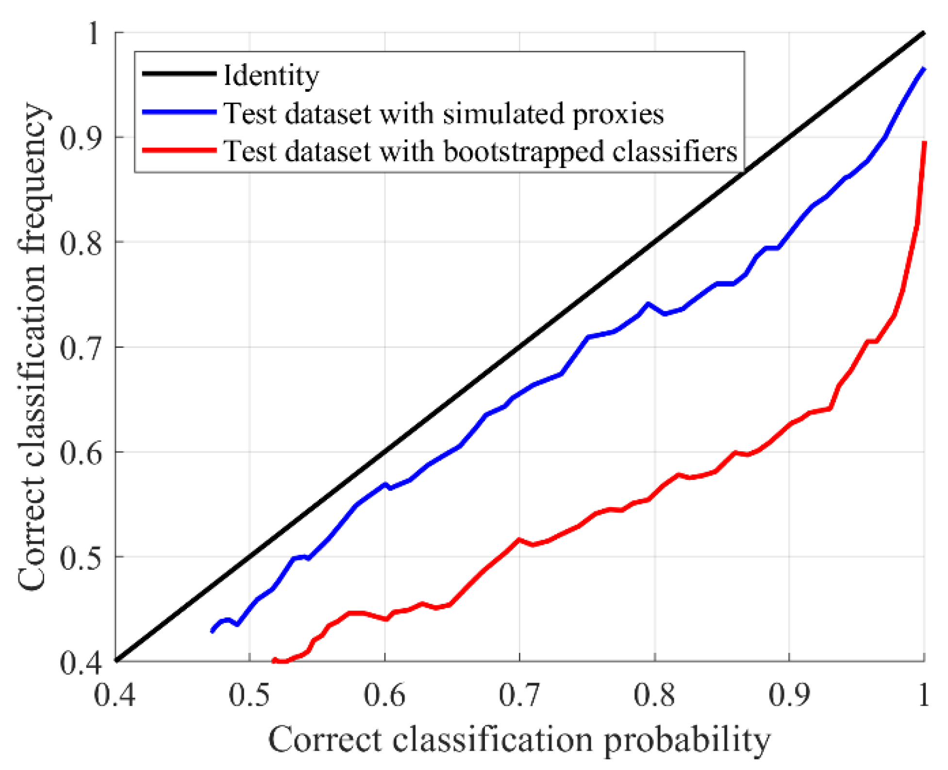
Risk-aware exploration decisions: By assessing the uncertainty in alteration predictions at each location, one can produce probability volumes for ore-bearing alteration type (read: probabilistic prospectivity maps). The implication is a better grasp of risk: areas with consistent predictions across scenarios are robust and could be trusted for decision-making, whereas areas with a high potential of ore-bearing alteration but uncertain predictions might need additional drilling for data acquisition to improve model reliability and reduce exploration risks. Confidence levels above $70\%$ are generally considered acceptable for geological classification tasks, while confidence levels below this threshold may indicate excessive uncertainty; more conservative thresholds may be justified for class assignment especially when economic consequences are high. Uncertainty-aware models can furthermore guide how to prioritize exploration targets according to the exploration program and risk preferences of the project developers (e.g., junior or major mining company) [70]. For instance, in advanced exploration stages, drilling programs may focus on those critical areas where the scenarios flip between ore-bearing and non-mineralized alteration classes, whereas other areas may be deprioritized as the additional data would not substantially impact project valuation. This approach contrasts with traditional geometry-based drilling plans, facilitating more cost-effective and risk-aligned programs, and ultimately reducing drilling requirements by focusing on uncertainty-informed target areas.

3.

Geological modeling: In ore geology research, geological models of alteration, lithology, and mineralization provide a quantitative basis to discuss the geometry of hydrothermal systems and can be used to test genetic hypotheses, for example, checking if the spatial distribution of predicted alteration aligns with expected fluid flow patterns or metal zoning. Our approach can generate multiple geological models, which AI can then analyze for spatial patterns consistent with mineral system theory. Mineral system modeling platforms (e.g., those that simulate fluid flow, heat transport, or geochemical dispersion) can incorporate the simulation outputs as stochastic priors for permeability, lithology, or structural features. This is complementary to current practices in mineral resource estimation where geostatistical simulation is used to quantify ore grade uncertainty—here we would quantify geological interpretation uncertainty.

4.

Mineral resource estimation: Assessing the uncertainty in the classification of alteration, lithology, or mineralization also supports probabilistic resource quantification, improves the efficiency of resource delineation, and enables scenario-based planning and more defensible reporting of mineral resources.

5.

Geometallurgical planning: Different alterations imply different ore hardness and processing characteristics. A 3D alteration model can outline geometallurgical domains (hard vs. soft ore, acid-consuming gangue, metallurgical recovery, sedimentation velocity, etc.), bridging geology and metallurgy.

7. Concluding Remarks

This study is significant on multiple fronts. Methodologically, it pushes the boundary by uniting geostatistical simulation with ML classification in a 3D geological context—an approach only hinted at in emerging literature. In terms of application, it delivered a high-accuracy alteration model that proved its worth in real-world exploration decisions, thus validating the approach’s utility. Compared to existing research in mineral exploration and ore geology, it achieves higher predictive performance and provides a template for how to handle incomplete and noisy data sets in complex 3D environments.

The use of simulated proxies stands out as a clever strategy to overcome limited and noisy regionalized data, likely setting a precedent for future 3D geological modeling. The implications are far-reaching: We are looking at the future of exploration where geologists augment their expertise with machine learning models that continuously learn from and interpolate between sparse data points, leading to faster and more accurate targeting of mineral resources. Geostatistical simulation furthermore injects uncertainty awareness into ML and AI workflows, making exploration decisions more risk-informed. This synergy of human and artificial intelligence, underpinned by sound geological reasoning and statistical rigor, could significantly improve success rates and efficiency in finding and developing orebodies going forward.

We expect more researchers and practitioners to adopt similar techniques for various tasks: not just alteration mapping, but also lithology logging from geochemical proxies, structural zone classification, or even regional prospectivity modeling in 2D or 3D. As computing power and software user-friendliness improve, junior exploration companies and large mining firms alike may start integrating these tools into their standard workflow-effectively bringing “Big Data” analytics into the core of geological modeling.

References

- Deb, M.; Sarkar, S. Minerals and Allied Natural Resources and Their Sustainable Development; Springer: Singapore, 2017. [Google Scholar]
- Robb, L. Introduction to Ore-Forming Processes; Blackwell Publishing: Oxford, UK, 2005. [Google Scholar]
- Guilbert, J.; Park, C. The Geology of Ore Deposits; W.H. Freeman and Company: New York, NY, USA, 1986. [Google Scholar]
- Barnes, H. Geochemistry of Hydrothermal Ore Deposits; John Wiley & Sons: New York, NY, USA, 1997. [Google Scholar]
- Lowell, J.; Guilbert, J. Lateral and vertical alteration mineralization zoning in porphyry ore deposits. Econ. Geol. 1970, 65, 373–408. [Google Scholar] [CrossRef]
- Mathieu, L. Quantifying hydrothermal alteration: A review of methods. Geosciences 2018, 8, 245. [Google Scholar] [CrossRef]
- Dutta, P.; Emery, X. Classifying rock types by geostatistics and random forests in tandem. Mach. Learn. Sci. Technol. 2024, 5, 025013. [Google Scholar] [CrossRef]
- Smirnoff, A.; Boisvert, E.; Paradis, S.J. Support vector machine for 3D modelling from sparse geological information of various origins. Comput. Geosci. 2008, 34, 127–143. [Google Scholar] [CrossRef]
- Abbaszadeh, M.; Hezarkhani, A.; Soltani-Mohammadi, S. Classification of alteration zones based on whole-rock geochemical data using support vector machine. J. Geol. Soc. India 2015, 85, 500–508. [Google Scholar] [CrossRef]
- Rodriguez-Galiano, V.; Sanchez-Castillo, M.; Chica-Olmo, M.; Chica-Rivas, M. Machine learning predictive models for mineral prospectivity: An evaluation of neural networks, random forest, regression trees and support vector machines. Ore Geol. Rev. 2015, 71, 804–818. [Google Scholar] [CrossRef]
- Caté, A.; Schetselaar, E.; Mercier-Langevin, P.; Ross, P. Classification of lithostratigraphic and alteration units from drillhole lithogeochemical data using machine learning: A case study from the Lalor volcanogenic massive sulphide deposit, Snow Lake, Manitoba, Canada. J. Geochem. Explor. 2018, 188, 216–228. [Google Scholar] [CrossRef]
- Xiang, J.; Xiao, K.; Carranza, E.J.M.; Chen, J.; Li, S. 3D mineral prospectivity mapping with random forests: A case study of Tongling, Anhui, China. Nat. Resour. Res. 2019, 29, 395–414. [Google Scholar] [CrossRef]
- Chen, J.; Mao, X.; Deng, H.; Liu, Z.; Wang, Q. Three-dimensional modelling of alteration zones based on geochemical exploration data: An interpretable machine-learning approach via generalized additive models. Appl. Geochem. 2020, 123, 104781. [Google Scholar] [CrossRef]
- Dumakor-Dupey, N.K.; Arya, S. Machine learning—A review of applications in mineral resource estimation. Energies 2021, 14, 4079. [Google Scholar] [CrossRef]
- Jooshaki, M.; Nad, A.; Michaux, S. A systematic review on the application of machine learning in exploiting mineralogical data in mining and mineral industry. Minerals 2021, 11, 816. [Google Scholar] [CrossRef]
- Jung, D.; Choi, Y. Systematic review of machine learning applications in mining: Exploration, exploitation, and reclamation. Minerals 2021, 11, 148. [Google Scholar] [CrossRef]
- Jia, R.J.; Lv, Y.; Wang, G.; Carranza, E.J.M.; Chen, Y.; Wei, C.; Zhang, Z. A stacking methodology of machine learning for 3D geological modeling with geological-geophysical datasets, Laochang Sn camp, Gejiu (China). Comput. Geosci. 2021, 151, 104754. [Google Scholar] [CrossRef]
- Pour, A.B.; Harris, J.; Zuo, R. Machine learning for analysis of geo-exploration data. In Geospatial Analysis Applied to Mineral Exploration; Pour, A.B., Parsa, M., Eldosouky, A.M., Eds.; Elsevier: Amsterdam, The Netherlands, 2023; pp. 279–294. [Google Scholar]
- Shi, Z.; Zuo, R.; Zhou, B. Deep reinforcement learning for mineral prospectivity mapping. Math. Geosci. 2023, 55, 773–797. [Google Scholar] [CrossRef]
- Farhadi, S.; Tatullo, S.; Konari, M.B.; Afzal, P. Evaluating StackingC and ensemble models for enhanced lithological classification in geological mapping. J. Geochem. Explor. 2024, 260, 107441. [Google Scholar] [CrossRef]
- Sun, K.; Chen, Y.; Geng, G.; Lu, Z.; Zhang, W.; Song, Z.; Guan, J.; Zhao, Y.; Zhang, Z. A review of mineral prospectivity mapping using deep learning. Minerals 2024, 14, 1021. [Google Scholar] [CrossRef]
- Gy, P. Sampling of Particulate Materials: Theory and Practice; Elsevier: Amsterdam, The Netherlands, 1982. [Google Scholar]
- Chilès, J.; Delfiner, P. Geostatistics: Modeling Spatial Uncertainty; John Wiley & Sons: Hoboken, NJ, USA, 2012. [Google Scholar]
- Banerjee, S.; Carlin, B.; Gelfand, A. Hierarchical Modeling and Analysis for Spatial Data; CRC Press: Boca Raton, FL, USA, 2014. [Google Scholar]
- Zhang, C.; Zuo, R.; Xiong, Y. Detection of the multivariate geochemical anomalies associated with mineralization using a deep convolutional neural network and a pixel-pair feature method. Appl. Geochem. 2021, 130, 104994. [Google Scholar] [CrossRef]
- Zhang, S.; Carranza, E.J.M.; Wei, H.; Xiao, K.; Yang, F.; Xiang, J.; Xu, Y. Data-driven mineral prospectivity mapping by joint application of unsupervised convolutional auto-encoder network and supervised convolutional neural network. Nat. Resour. Res. 2021, 30, 1011–1031. [Google Scholar] [CrossRef]
- Behrens, T.; Schmidt, K.; Rossel, R.A.V.; Gries, P.; Scholten, T.; MacMillan, R.A. Spatial modelling with Euclidean distance fields and machine learning. Eur. J. Soil Sci. 2018, 69, 757–770. [Google Scholar] [CrossRef]
- Balk, B.; Elder, K. Combining binary decision tree and geostatistical methods to estimate snow distribution in a mountain watershed. Water Resour. Res. 2000, 36, 13–26. [Google Scholar] [CrossRef]
- Li, J.; Heap, A.D.; Potter, A.; Daniell, J.J. Application of machine learning methods to spatial interpolation of environmental variables. Environ. Model. Softw. 2011, 26, 1647–1659. [Google Scholar] [CrossRef]
- Fayad, I.; Baghdadi, N.; Bailly, J.; Barbier, N.; Gond, V.; Hérault, B.; El Hajj, M.; Fabre, F.; Perrin, J. Regional scale rain-forest height mapping using regression-kriging of spaceborne and airborne LiDAR data: Application on French Guiana. Remote Sens. 2016, 8, 240. [Google Scholar] [CrossRef]
- Liu, Y.; Cao, G.; Zhao, N.; Mulligan, K.; Ye, X. Improve ground-level PM2.5 concentration mapping using a random forests-based geostatistical approach. Environ. Pollut. 2018, 235, 272–282. [Google Scholar] [CrossRef]
- Fox, E.; Ver Hoef, J.; Olsen, A.R. Comparing spatial regression to random forests for large environmental data sets. PLoS ONE 2020, 15, e0229509. [Google Scholar] [CrossRef]
- Schmidinger, J.; Barkov, V.; Vogel, S.; Atzmueller, M.; Heuvelink, G.B.M. Kriging prior regression: A case for kriging-based spatial features with TabPFN in soil mapping. arXiv 2025, arXiv:2509.09408v2. [Google Scholar]
- Saha, A.; Basu, S.; Datta, A. Random forests for spatially dependent data. J. Am. Stat. Assoc. 2023, 118, 665–683. [Google Scholar] [CrossRef]
- Hengl, T.; Nussbaum, M.; Wright, M.; Heuvelink, G.; Gräler, B. Random forest as a generic framework for predictive modeling of spatial and spatio-temporal variables. PeerJ 2018, 6, e5518. [Google Scholar] [CrossRef]
- Georganos, S.; Grippa, T.; Niang Gadiaga, A.; Linard, C.; Lennert, M.; Vanhuysse, S.; Mboga, N.; Wolff, E.; Kalogirou, S. Geographical random forests: A spatial extension of the random forest algorithm to address spatial heterogeneity in remote sensing and population modelling. Geocarto Int. 2021, 36, 121–136. [Google Scholar] [CrossRef]
- Qin, Z.; Peng, Q.; Jin, C.; Xu, J.; Xing, S.; Zhu, P.; Yang, G. Geographically weighted random forest fusing multi-source environmental covariates for spatial prediction of soil heavy metals. Environ. Pollut. 2025, 385, 127135. [Google Scholar] [CrossRef] [PubMed]
- Sekulić, A.; Kilibarda, M.; Heuvelink, G.B.M.; Nikolić, M.; Bajat, B. Random forest spatial interpolation. Remote Sens. 2020, 12, 1687. [Google Scholar] [CrossRef]
- Talebi, H.; Peeters, L.J.M.; Otto, A.; Tolosana-Delgado, R. A truly spatial random forests algorithm for geoscience data analysis and modelling. Math. Geosci. 2022, 54, 1–22. [Google Scholar] [CrossRef]
- Nwaila, G.T.; Zhang, S.E.; Frimmel, H.E.; Manzi, M.S.D.; Dohm, C.; Durrheim, R.J.; Burnett, M.; Tolmay, L. Local and target exploration of conglomerate-hosted gold deposits using machine learning algorithms: A case study of the Witwatersrand gold ores, South Africa. Nat. Resour. Res. 2020, 29, 135–159. [Google Scholar] [CrossRef]
- Erten, G.E.; Yavuz, M.; Deutsch, C.V. Combination of machine learning and kriging for spatial estimation of geological attributes. Nat. Resour. Res. 2022, 31, 191–213. [Google Scholar] [CrossRef]
- Adeli, A.; Emery, X.; Dowd, P. Geological modelling and validation of geological interpretations via simulation and classification of quantitative covariates. Minerals 2018, 8, 7. [Google Scholar] [CrossRef]
- Talebi, H.; Mueller, U.; Tolosana-Delgado, R.; Grunsky, E.; McKinley, J.; de Caritat, P. Surficial and deep earth material prediction from geochemical compositions. Nat. Resour. Res. 2019, 28, 869–891. [Google Scholar] [CrossRef]
- Bai, T.; Tahmasebi, P. Hybrid geological modeling: Combining machine learning and multiple-point statistics. Comput. Geosci. 2020, 142, 104519. [Google Scholar] [CrossRef]
- Chen, T.; Guestrin, C. XGBoost: A scalable tree boosting system. In Proceedings of the KDD ’16: The 22nd ACM SIGKDD International Conference on Knowledge Discovery and Data Mining, San Francisco, CA, USA, 13–17 August 2016; Krishnapuram, B., Shah, M., Eds.; Association for Computing Machinery: New York, NY, USA, 2016; pp. 785–794. [Google Scholar]
- Friedman, J.H. Greedy function approximation: A gradient boosting machine. Ann. Stat. 2001, 29, 1189–1232. [Google Scholar] [CrossRef]
- Domingos, P. MetaCost: A general method for making classifiers cost-sensitive. In Proceedings of the KDD ’99: The Fifth ACM SIGKDD International Conference on Knowledge Discovery and Data Mining, San Diego, CA, USA, 15–18 August 1999; Fayyad, U., Chaudhuri, S., Madigan, D., Eds.; Association for Computing Machinery: New York, NY, USA, 1999; pp. 155–164. [Google Scholar]
- Efron, B. Bootstrap methods: Another look at the jackknife. Ann. Stat. 1979, 7, 101–118. [Google Scholar] [CrossRef]
- Wackernagel, H. Multivariate Geostatistics: An Introduction with Applications; Springer: Berlin/Heidelberg, Germany, 2003. [Google Scholar]
- Lantuéjoul, C. Geostatistical Simulation: Models and Algorithms; Springer: Berlin/Heidelberg, Germany, 2002. [Google Scholar]
- Shwartz-Ziv, R.; Armon, A. Tabular data: Deep learning is not all you need. Inf. Fusion 2022, 81, 84–90. [Google Scholar] [CrossRef]
- Li, H.; Gao, M.; Ji, X.; Zhang, Z.; Cheng, Z.; Santosh, M. Machine learning-based tectonic discrimination using basalt element geochemical data: Insights into the Carboniferous-Permian tectonic regime of western Tianshan orogen. Minerals 2025, 15, 122. [Google Scholar] [CrossRef]
- Adeli, A.; Emery, X. Geostatistical simulation of rock physical and geochemical properties with spatial filtering and its application to predictive geological mapping. J. Geochem. Explor. 2021, 220, 106661. [Google Scholar] [CrossRef]
- Guartán, J.A.; Emery, X. Regionalized classification of geochemical data with filtering of measurement noises for predictive lithological mapping. Nat. Resour. Res. 2021, 30, 1033–1052. [Google Scholar] [CrossRef]
- Emery, X.; Arroyo, D.; Porcu, E. An improved spectral turning-bands algorithm for simulating stationary vector Gaussian random fields. Stoch. Environ. Res. Risk Assess. 2016, 30, 1863–1873. [Google Scholar] [CrossRef]
- Yakubchuk, A.; Cole, A.; Seltmann, R.; Vitalievich, S.V. Tectonic setting, characteristics, and regional exploration criteria for gold mineralization in the Altaid orogenic collage: The Tien Shan Province as a key example. In Integrated Methods for Discovery: Global Exploration in Twenty-First Century; Goldfarb, R.J., Nielsen, R.L., Eds.; Society of Economic Geologists: Littleton, CO, USA, 2002; pp. 177–201. [Google Scholar]
- Seedorff, E.; Dilles, J.H.; Proffett, J.M.; Einaudi, M.T.; Zurcher, L.; Stavast, W.J.A.; Johnson, D.A.; Barton, M.D. Porphyry deposits: Characteristics and origin of hypogene features. In Economic Geology One Hundredth Anniversary Volume; Hedenquist, J.W., Thompson, J.F.H., Goldfarb, R.J., Richards, J.P., Eds.; Society of Economic Geologists: Littleton, CO, USA, 2005; pp. 251–298. [Google Scholar]
- Sillitoe, R.H. Porphyry copper systems. Econ. Geol. 2010, 105, 3–41. [Google Scholar] [CrossRef]
- Porter, T. The geology, structure and mineralisation of the Oyu Tolgoi porphyry copper-gold-molybdenum deposits, Mongolia: A review. Geosci. Front. 2016, 7, 375–407. [Google Scholar] [CrossRef]
- Emery, X. Iterative algorithms for fitting a linear model of coregionalization. Comput. Geosci. 2010, 36, 1150–1160. [Google Scholar] [CrossRef]
- Zhang, S.; Nwaila, G.; Bourdeau, J.; Ghorbani, Y.; Carranza, E. Machine learning-based delineation of geodomain boundaries: A proof-of-concept study using data from the Witwatersrand goldfields. Nat. Resour. Res. 2023, 32, 879–900. [Google Scholar] [CrossRef]
- Chen, X.; Warner, T.A.; Campagna, D.J. Integrating visible, near-infrared and short-wave infrared hyperspectral and multispectral thermal imagery for geological mapping at Cuprite, Nevada: A rule-based system. Int. J. Remote Sens. 2010, 31, 1733–1752. [Google Scholar] [CrossRef]
- Bishop, C.A.; Liu, J.G.; Mason, P.J. Hyperspectral remote sensing for mineral exploration in Pulang, Yunnan Province, China. Int. J. Remote Sens. 2011, 32, 2409–2426. [Google Scholar] [CrossRef]
- Pour, A.B.; Hashim, M. ASTER, ALI and Hyperion sensors data for lithological mapping and ore minerals exploration. SpringerPlus 2014, 3, 130. [Google Scholar] [CrossRef]
- Alimohammadi, M.; Alirezaei, S.; Kontak, D.J. Application of ASTER data for exploration of porphyry copper deposits: A case study of Daraloo–Sarmeshk area, southern part of the Kerman copper belt, Iran. Ore Geol. Rev. 2015, 33, 183–199. [Google Scholar] [CrossRef]
- Canbaz, O.; Gürsoy, O.; Karaman, M.; Çalışkan, A.B.; Gökce, A. Hydrothermal alteration mapping using EO-1 Hyperion hyperspectral data in Kosedag, Central Eastern Anatolia (Sivas-Turkey). Arab. J. Geosci. 2021, 14, 2245. [Google Scholar] [CrossRef]
- Madani, N.; Emery, X. A comparison of search strategies to design the cokriging neighborhood for predicting coregionalized variables. Stoch. Environ. Res. Risk Assess. 2019, 33, 183–199. [Google Scholar] [CrossRef]
- Babak, O.; Deutsch, C.V. Collocated cokriging based on merged secondary attributes. Math. Geosci. 2009, 41, 921–926. [Google Scholar] [CrossRef]
- Liang, M.; Putzmann, C.; Gokaydin, D. Enhancing Geoscience Model Confidence via Digital Twins—Integrated Modelling, Simulation, and Machine Learning Technologies; The Australasian Institute of Mining and Metallurgy: Carlton, VIC, Australia, 2024. [Google Scholar]
- Cáceres, A.; Emery, X.; Ibarra, F.; Pérez, J.; Seguel, S.; Fuster, G.; Pérez, A.; Riquelme, R. A stochastic framework for mineral resource uncertainty quantification and management at Compañía Minera Doña Inés de Collahuasi. Minerals 2025, 15, 855. [Google Scholar] [CrossRef]