Article

A Hybrid Framework for Detecting Gold Mineralization Zones in G.R. Halli, Western Dharwar Craton, Karnataka, India

by
P. V. S. Raju
1,*,
Venkata Sai Mudili
2 and
Avatharam Ganivada
2
1
Council of Scientific and Industrial Research (CSIR)-National Geophysical Research Institute, Hyderabad 500007, India
2
School of Computer and Information Sciences, University of Hyderabad, Hyderabad 500046, India
*
Author to whom correspondence should be addressed.
Minerals 2025, 15(11), 1125; https://doi.org/10.3390/min15111125
Submission received: 2 September 2025 / Revised: 13 October 2025 / Accepted: 13 October 2025 / Published: 28 October 2025

Abstract

Mineral prospectivity mapping (MPM) is a powerful approach for identifying mineralization zones with high potential for economically viable mineral deposits. This study proposes a hybrid framework combining a Wasserstein Generative Adversarial Network with Gradient Penalty (WGAN-GP), a Convolutional Neural Network (CNN) and a Fuzzy-Kernel Extreme Learning Machine (FKELM) to address the challenges of imbalanced and uncertain datasets in mineral exploration. The approach was applied to the G.R. Halli gold prospect, in the Chitradurga Schist Belt, Western Dharwar Craton, India, using nine geochemical pathfinder elements. WGAN-GP generated high-quality negative samples, balancing the dataset and reducing overfitting. Compared with Support Vector Machines, Gradient Boosting, and a baseline CNN, FKELM (AUC = 0.976, accuracy = 92%) and WGAN-GP + CNN (AUC = 0.973, accuracy = 91%) showed superior performance and produced geologically coherent prospectivity maps. Promising gold targets were delineated, closely aligned with known mineralized zones and geochemical anomalies. This hybrid framework provides a robust, cost-effective, and scalable MPM solution for structurally controlled geological tracts, insufficient data terrains, and integration with additional geoscience datasets for other complex mineral systems.

1. Introduction

Mineral prospectivity mapping (MPM) is a key tool in mineral exploration, designed to identify regions with high potential for economically viable deposits. It integrates multiple geoscientific datasets—geological, geochemical, and geophysical—into the spatial models of mineralization. Traditionally, MPM has relied on approaches such as fuzzy logic, but these methods face limitations, including data imbalance, high dimensionality, and uncertainty [1].
Recent advances in machine learning (ML) and deep learning (DL) offer powerful alternatives. These methods can model complex and imbalanced datasets by learning hidden patterns and spatial relationships [2,3]. However, their application in mineral exploration is hindered by the scarcity of labeled data—especially positive samples. This often leads to overfitting and reduced generalizability. The strong imbalance between mineralized and non-mineralized zones further challenges model robustness and reliability.
To address these limitations, this study applies data augmentation techniques—especially Generative Adversarial Networks (GANs)—to generate negative samples. Specifically, it uses a Wasserstein GAN with Gradient Penalty (WGAN-GP). This offers improved training stability and higher-quality sample generation [4]. Augmenting the dataset with these samples yields a more balanced training set. This improves the predictive performance of Deep Learning (DL) models in MPM.
This methodology is applied to gold exploration in the G.R. Halli prospect, located within the Chitradurga Schist Belt, Western Dharwar Craton, Karnataka, India. Gold mineralization in this region is mainly associated with structurally controlled quartz–sulfide veins and shear zones in Archaean greenstone belts. Despite its high mineralization potential, the area remains underexplored due to complex structural and lithological conditions, making robust MPM crucial for guiding cost-effective field exploration.
While DL has been applied to MPM in recent studies, most models struggle with data imbalances during classification, and GAN-based approaches are still rare in geoscience. There is also a gap in integrating DL with Machine Learning (ML) models that can handle imbalanced data. To bridge this gap, this study proposes a hybrid framework combining the WGAN-GP CNN model with a Fuzzy Kernel Extreme Learning Machine (FKELM) known for its robustness under imbalanced conditions [4,5,6,7].
Additionally, a comparative analysis is performed using support vector machines (SVM), gradient boosting (GB), and a baseline Convolution Neural Network (RCNN) [8]. Model performance is evaluated based on classification accuracy, area under curve (AUC) scores, and spatial correspondence with known mineralized zones. This approach not only validates model effectiveness but also establishes a foundation for future MPM studies.
The objectives of this study are as follows:
  • Generate anomaly maps of selected geochemical elements using ArcGIS.
  • Create a negative sample dataset by defining non-mineralized zones based on criteria derived from the positive dataset.
  • Construct a spatial distribution map from positive and negative datasets.
  • Evaluate model performance using classification accuracy, AUC values, and ROC curves.
  • Predict spatial probabilities of mineral prospectivity for various classifiers.
  • Develop and compare the MPMs generated by both the ML and DL models.
This work advances research on efficient ML/DL frameworks for mineral exploration, particularly under geologically complex and imbalanced data conditions.

2. Literature Review

In recent years, applying ML and DL models to mineral prospectivity mapping (MPM) has addressed the key limitations of traditional approaches, such as fuzzy and weighted methods [1]. While these conventional methods offer interpretability, they struggle with imbalanced, uncertain, and high-dimensional geoscientific datasets [1]. ML models such as Support Vector Machines (SVM) and Gradient Boosting (GB) have proven effective in capturing nonlinear/complex spatial patterns [8,9,10]. DL models like Convolutional Neural Networks (CNNs) further improve the learning of complex spatial relationships [3]. A major challenge, however, is the imbalance between mineralized and non-mineralized samples, which often leads to overfitting and poor model generalization [2]. To address this, recent studies have used data augmentation techniques, including Generative Adversarial Networks (GANs), to generate synthetic negative samples.
Among these, the Wasserstein GAN with Gradient Penalty (WGAN-GP) has shown improved training stability and more realistic sample generation under class imbalance [4]. While GANs have been applied in geoscience for tasks like hyperspectral data simulation and lithological image enhancement [11,12], their use in augmenting negative sample data in MPM remains rare.
Hybrid learning models that combine fuzzy logic with kernel-based algorithms are increasingly used to address uncertainty in spatial datasets. The Fuzzy Kernel Extreme Learning Machine (FKELM) enables rapid training and effectively handles unclear class boundaries [5,6,7]. Although the combined use of GAN-based negative sample augmentation with CNN and FKELM models has not been applied to MPM, this study evaluates WGAN-GP CNN and FKELM independently to establish a foundation for future geoscience research.
The G R Halli in Chitradurga Schist Belt, western Dharwar craton, India is a well-known but underexplored mineralization zone, characterized by structural complexity. Applying advanced data-driven models can help to identify potential mineralized locations, reducing field exploration costs and improving targeting accuracy.
This study proposes a new framework integrating WGAN-GP with CNN and FKELM models to generate MPMs. The approach aims to enhance spatial prediction accuracy and model stability under complex, imbalanced dataset conditions, leading to more effective MPM.

3. Geology of the Area

Geology of Dharwar Craton

The Indian shield comprises three primary proto-continents: Bundelkhand, Aravalli, and Dharwar–Singhbhum [13,14]. Within the Dharwar–Singhbhum proto-continent, the Karnataka and Singhbhum nuclei (KN and SN) consist of rocks older than 2.5 Ga, forming part of the Archaean continental crust of the South Indian shield, which has been extensively studied [15].
Among these regions, the Dharwar craton is the most thoroughly investigated, constituting a significant portion of the Dharwar–Singhbhum proto-continent, and represents an advanced stage of cratonization [16,17,18,19,20,21,22,23,24,25,26,27].
It is one of the largest Archean crustal blocks in South India, with lithological units up to 3.6 Ga [28]. The Craton is bounded by the Narmada–Son–Godavari rift system to the north–northeast, the western margin to the west, the Eastern Ghat Mobile Belt to the east, and the granulite terrain to the south, separated by a transition zone (Figure 1A). The Craton was originally divided into western and eastern blocks [29], later renamed the Western Dharwar Craton (WDC) and the Eastern Dharwar Craton (EDC) [24].
The WDC and EDC are separated by the Chitradurga granite near the eastern margin of the Chitradurga schist belt and the western margin of the Closepet granite. These two blocks show distinct differences in regional geology, lithological units, and metamorphic grade, which are beyond the scope of this paper but are discussed elsewhere [30,31,32].
In the western Dharwar Craton, the main Chitradurga Schist Belt extends from Gadag to Srirangapatna over a strike length of ~450 km, trending NNW-SSE. It exhibits upper greenschist facies metamorphism in its northern and central portions, grading to amphibolitic facies along the flanks and in the south. The belt largely comprises the Chitradurga Group of the younger Dharwar Supergroup, with subordinate Bababudan and Sargur Group rocks. The Chitradurga Group consists mainly of chemogenic detrital sediments and associated volcanics, represented in ascending order by the Vanivilas, Ingaldhal, and Hiriyur Formations.
The G. R. Halli area consists of rocks from the Ingaldhal Formation (2.9–2.55 Ga), bounded by the Chitradurga Granites to the west and the Hiriyur Formation to the east, separated by the G.R. Halli conglomerate. The TTG (tonalite–trondhjemite–granodiorite) basement is exposed farther east. Major litho-units include grayish-green, massive to schistose metabasalt interlayered with greywacke and meta-argillite/phyllite. These rocks are intruded by metabasic dykes and sills, quartz–carbonate veins, and quartz veins. Wall rock alterations, particularly carbonatization, sericitization, and chloritization, are widespread around the mineralized zones, with the unaltered massive metabasalt to the west serving as a marker for halos of alteration.
Hydrothermal wall rock alteration has extensively overprinted both pre-metamorphic and, in part, metamorphic mineral assemblages. Previous studies identified carbonatization, sericitization, and chloritization as the dominant alteration types around the G. R. Halli deposit [33].
This study documents systematic alteration assemblages from proximal to distal zones of the deposit, including the following:
  • Quartz veins in altered metabasalt and meta-argillite/phyllite.
  • Lenses or zones rich in ankeritic veins.
  • Quartz–sericite assemblages.
  • Chlorite + ankerite + quartz + albite + Na-mica (paragonite) assemblages.
  • Quartz + ankerite + tourmaline ± albite assemblages.
Among these, ankerite-dominant alterations are the most distinctive and widespread, occurring in both proximal and distal parts of the mineralized system. Carbonatization affects nearly all litho-units, whereas the chlorite + ankerite + quartz + albite + paragonite assemblage is spatially restricted to the southern sectors of distal-to-near-proximal zones. Paragonite is most recorded in the southern, southeastern, and southwestern margins, 160–750 m from adit 2.
Borehole data confirms that the associated shear zones dip moderately to steeply. Within these shears, minor and mesoscopic F1 and F2 folds are well developed, typically appearing stretched parallel to the shear orientation. The arcuate and curvilinear geometry of the shears is interpreted through F3 cross-folding, indicating that shearing occurred synchronously with, or after, the F2 deformational event.
Gold (Au), silver (Ag), copper (Cu), lead (Pb), zinc (Zn), cobalt (Co), nickel (Ni), arsenic (As), antimony (Sb), tellurium (Te), selenium (Se), and mercury (Hg) are key geochemical pathfinders in gold exploration. Archaean gold ores are typically gold-rich and variably enriched in Ag, As, tungsten (W), Sb, bismuth (Bi), and Pb. When anomalies of several of these elements coincide and align with geological evidence, the probability of discovering gold increases significantly.
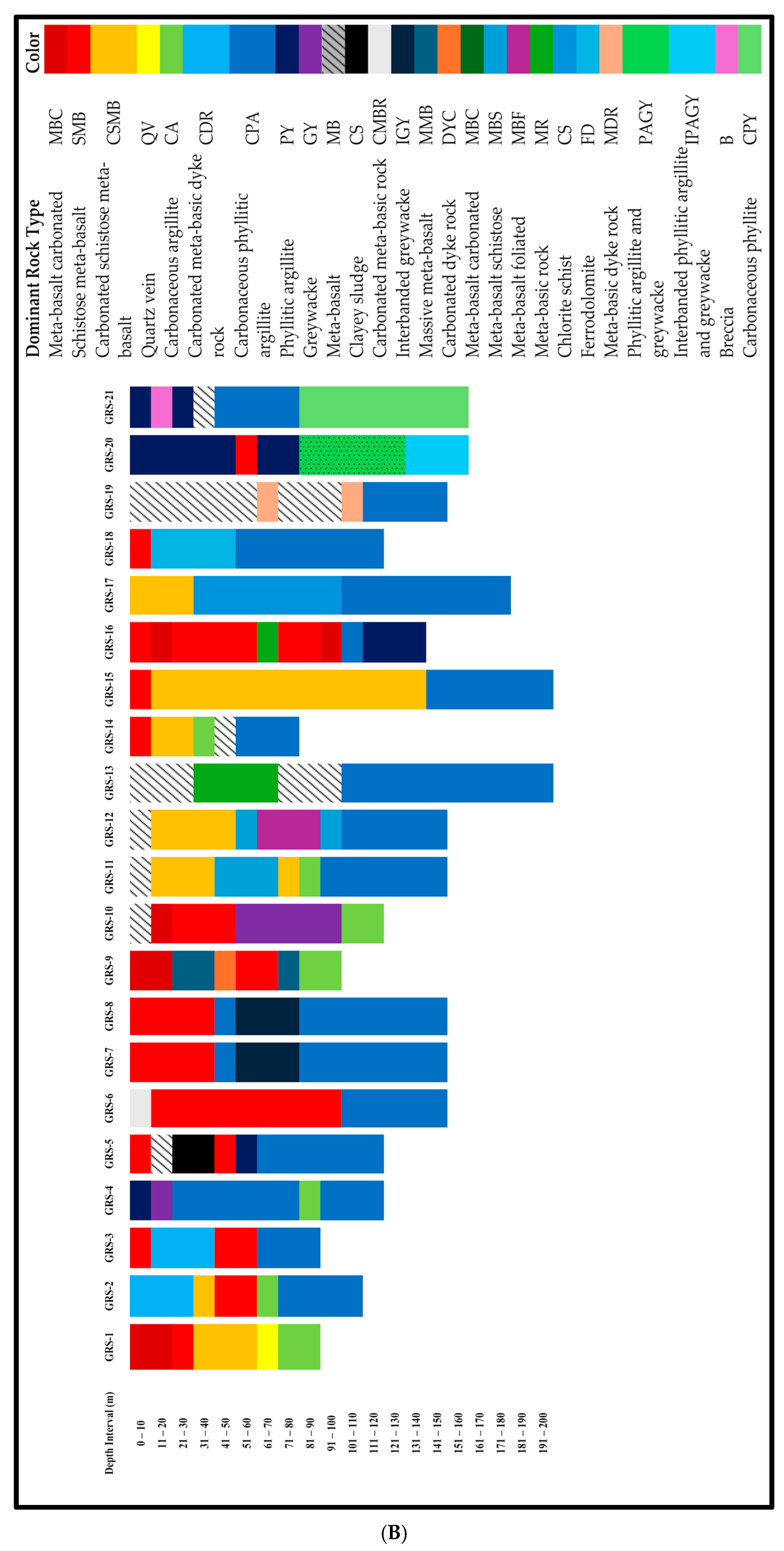
In India, geochemical explorations for gold have been limited in number, with most investigations relying more on trenching and drilling. Details on the types of lithologies in the boreholes are provided in Figure 1B. Arsenic is particularly important, as it occurs widely in sulfide minerals associated with polymetallic deposits, containing Co, Hg, Bi, Ag, V, Mo, and Au-Ag arsenide. Pathfinder elements, such as As, Sb, Te, W, and Bi, when analyzed in rocks, ores, alluvium, or groundwater, are valuable indicators for gold prospecting. A better understanding of As and Sb transport and deposition could further improve exploration success rates.

4. Methodology

This study developed a hybrid mineral prospectivity mapping (MPM) framework that integrates synthetic negative sample generation using Wasserstein Generative Adversarial Networks with Gradient Penalty (WGAN-GP) and classification with CNN and Fuzzy Kernel Extreme Learning Machine (FKELM) models. For comparison, Support Vector Machines (SVM) and Gradient Boosting (GB) and a baseline CNN were also implemented. The workflow follows standard geoscientific modeling practices [1,2,3,4,5,6,7,8,9], with all computations performed on Google Colab.

4.1. Data Preparation

Geochemical element concentration maps for copper (Cu), lead (Pb), zinc (Zn), nickel (Ni), cobalt (Co), antimony (Sb), arsenic (As), silver (Ag), and gold (Au) were selected as predictor variables:
x = Cu,Pb,Zn,Ni,Co,Sb,As,Ag,Au .
Samples were labeled as mineralized (y = 1) or non-mineralized (y = 0) based on borehole assay results and geological mapping. Positive and negative datasets were concatenated and split into training (70%) and testing (30%) sets using stratified sampling to preserve class ratios [2].
Feature scaling: All models except FKELM used Min–Max normalization:
x i j ~ = x i j min j | x j / max j | x j min j | x j
The FKELM applied additional z-score standardization [7]:
x i j ^ = x i j ~ μ j σ j ,
μ j and σ j represent mean and standard deviation, respectively.

4.2. Synthetic Data Generation Using WGAN-GP

To address class imbalance, a WGAN-GP [4] was used to generate synthetic negative samples.
Architecture:
  • Generator G: Input latent vector z ∈ R20 sampled from N(0, I). Layers: Linear(20, 64) → ReLU → Linear(64, 128) → ReLU → Linear(128, 9).
  • Critic D: Input x ∈ R9. Layers: Linear(9, 128) → LeakyReLU(0.2) → Linear(128, 64) → LeakyReLU(0.2) → Linear(64, 1).
Loss functions:
L D = E x ~ p g D x ~ E x p r D x + λ E x ^ p x ^ | x ^ D x ^ | 2 1 2
L G = E x ~ p g D x ~
where λ = 10 and x ^ = α x + 1 α x ~ , α U 0,1 .
Training settings: Adam optimizer η = 10 4 , β 1 = 0.0 , β 2 = 0.9 ; batch size 64; 1000 epochs. The negatives that were generated were appended to real positives to form a balanced CNN training set.

4.3. CNN Classification

A 1-D convolutional neural network [3] modeled nonlinear geochemical patterns.
Architecture: Input shape (1, 9), Conv1D(1, 32, kernel size = 3) → ReLU → Flatten → Linear(224, 64) → ReLU → Linear(64, 2).
Probability output:
p mineralized x = e s 1 / e s 0 + e s 1
where s 1 , s 2 are logits for classes 0 and 1.
Training settings were as follows: cross-entropy loss; Adam optimizer ( η = 0.001 0.003 ) ; batch size 8; 50 epochs.

4.4. Fuzzy-Kernel Extreme Learning Machine (FKELM)

FKELM integrates type-2 fuzzy logic and Gaussian kernels [5,7].
Type-2 fuzzy membership:
μ A x = x min x max x min x
μ upper = μ A infl , ° μ lower = μ A 1 / infl , infl = 0.9 .
Hamacher t-conorm aggregation:
μ = μ upper + μ lower + λ 2 μ upper μ lower 1 1 λ μ upper μ lower , λ = 3.5 .
Omega kernel:
Ω x i , x j = μ x i exp | x i x j | 2 2 σ 2 , σ = 1.0 .
The fuzzy Kernel function can be seen in [5].
ELM solution:
β = K + I C Y , C = 5000 .
Prediction:
p 1 ^ x = y 1 ^ y 0 ^ + y 1 ^ .

4.5. Machine Learning Models

Support vector machine (SVM): The SVM with a radial basis function (RBF) kernel seeks a decision function:
f x = sign ( i = 1 N α i y i K x i , x + b ) ,
where y i { 1 , 1 } are class labels, α i are Lagrange multipliers from the dual optimization, b is the bias term, and the RBF kernel is defined as follows:
K x i , x j = exp γ | x i x j | 2 .
with γ as the kernel width parameter. Probabilistic outputs are obtained via Platt scaling applied to the decision values.
Gradient boosting (GB): GB constructs an additive model of M regression trees:
F M x = m = 1 M ν h m x ,
where h m is the decision tree fitted at iteration m to the negative gradient of the loss function, and ν 0 , 1 is the learning rate. For binary classification with logistic loss:
l y , F x = log 1 + exp y F x
The predicted class probability is as follows:
p mineralized x = 1 1 + e F M x

4.6. Evaluation Metrics

The performance of the models was assessed using accuracy and area under the ROC curve (AUC) [2]:
Accuracy = 1 N i = 1 N I y ^ i = y i
AUC = 0 1 TPR FPR d FPR
ROC curves were computed for all models. Spatial prospectivity score maps were generated by applying models to geochemical data and exporting prediction scores for GIS overlay with known mineralized zones.

4.7. Hyperparameter Tuning Strategy

Model hyperparameters were initialized using values from [3,4,7] and refined via grid search with five-fold cross-validation. For WGAN-GP, tuning targeted the learning rate, gradient penalty coefficient (λ), and latent dimension size. CNN optimization focused on filter size, number of filters, and learning rate. FKELM parameters (σ, λ, inflation factor, and C) were selected to maximize mean AUC across folds. SVM and GB parameters were tuned using the same cross-validation strategy.

4.8. Workflow Summary

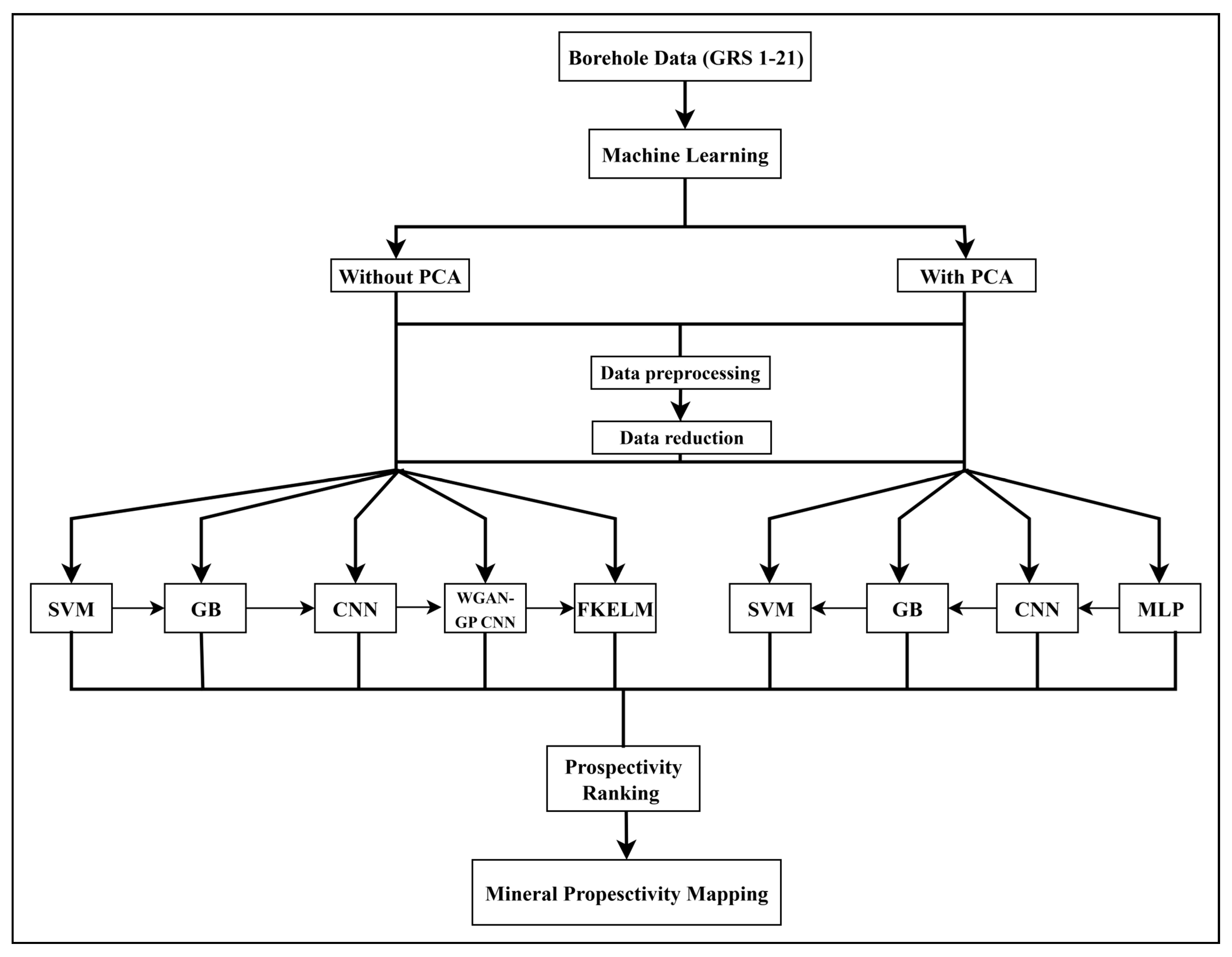
Figure 2 shows the complete MPM workflow, from data acquisition to map generation and spatial validation.

5. Results and Discussions

5.1. Data Preprocessing

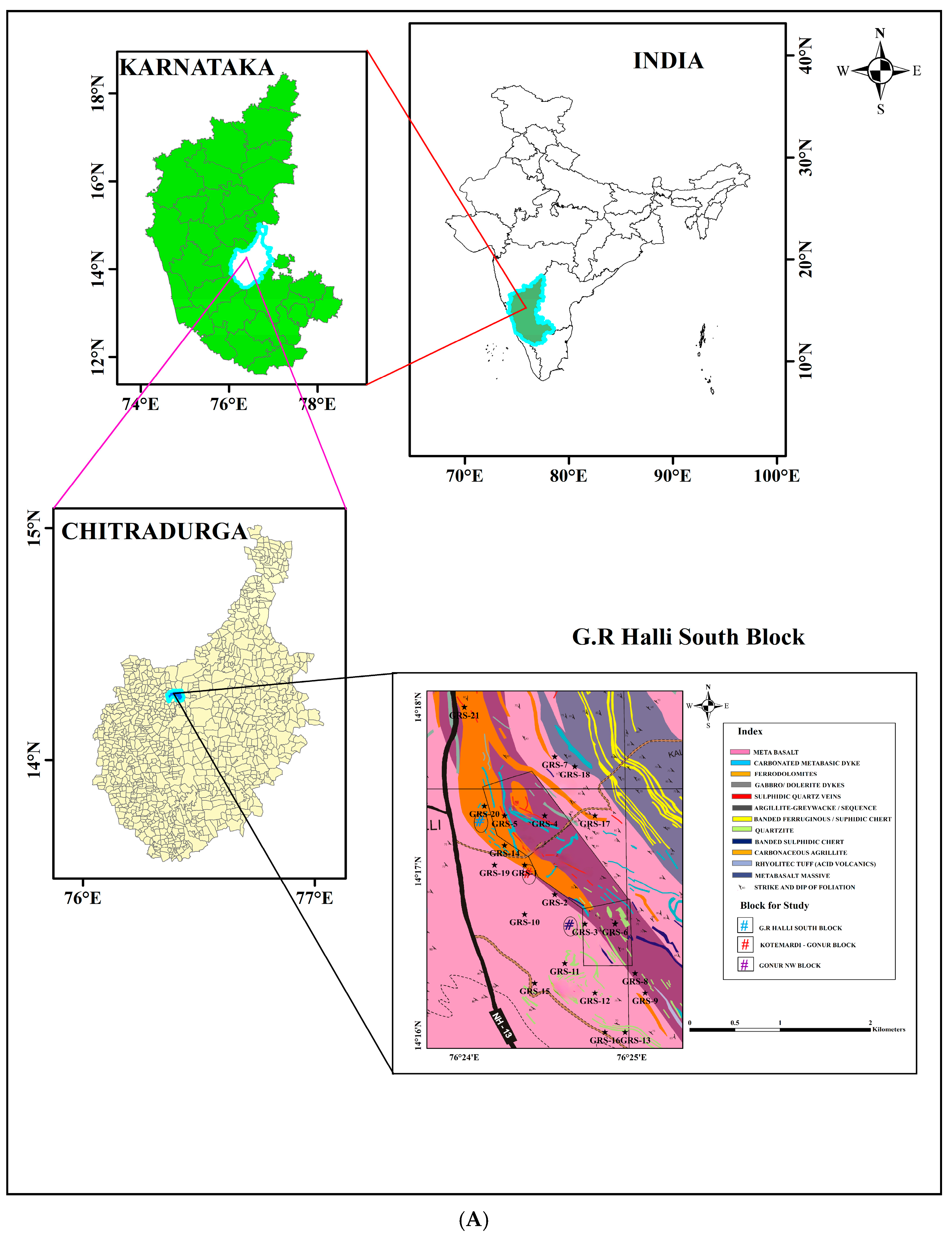
The study used 21 boreholes, each containing nine geochemical elements. The dataset was first examined for quality and consistency. Latitude and longitude values, originally presented in a local coordinate system, were converted to a geographic coordinate system (GCS) with decimal degrees for accurate spatial referencing. After the pre-processing, the dataset (.csv) was imported into ArcGIS 10.4, where borehole locations were geo-referenced and labeled sequentially from GRS-1 to GRS-21.
Geochemical element concentration maps were generated using the inverse distance weighting (IDW) interpolation (Arc Toolbox > Spatial Analyst Tools > Interpolation > IDW). This produced raster layers representing the spatial distribution of concentration of each element across the study area, as shown in the binary diagram (Figure 3 and Figure 4).
The geological map, as shown in Figure 5A,B, which maps the boreholes, illustrates the relationship between gold (Au) and lithologies, along with the pathfinder elements—arsenic (As), antimony (Sb), zinc (Zn), lead (Pb), silver (Ag), and copper (Cu)—which are commonly enriched in gold-bearing zones due to their shared geochemical behavior and ore-forming processes. Arsenic and antimony are strong indicators of gold in hydrothermal systems, particularly in orogenic and epithermal deposits. Zinc, lead, and silver often form geochemical halos around gold-bearing structures, typically within polymetallic sulfide systems. Copper, associated with porphyry and skarn-type deposits, reflects deep magmatic–hydrothermal activity that facilitates gold mobilization. The spatial distribution of these elements supports their genetic link with gold and their effectiveness as exploration guides.
Model training requires both positive (mineralized) and negative (non-mineralized) samples. In this study, positive samples came from 21 known borehole locations with latitude and longitude data. Negative samples were selected to balance the dataset using three main criteria: (1) sufficient distance from known ore deposits; (2) exclusion of areas with high concentrations of mineralization-related elements; and (3) even geographic distribution across the study area.
Based on these criteria, 21 negative samples which were nonmineralized were selected, yielding a dataset of 42 samples (21 positive and 21 negative). This dataset was split 70:30 into training and testing sets. The training set was used to learn the underlying structure of the patterns, while the testing set evaluated model performance and generalization ability.

5.2. WGAN-GP-Based Data Augmentation

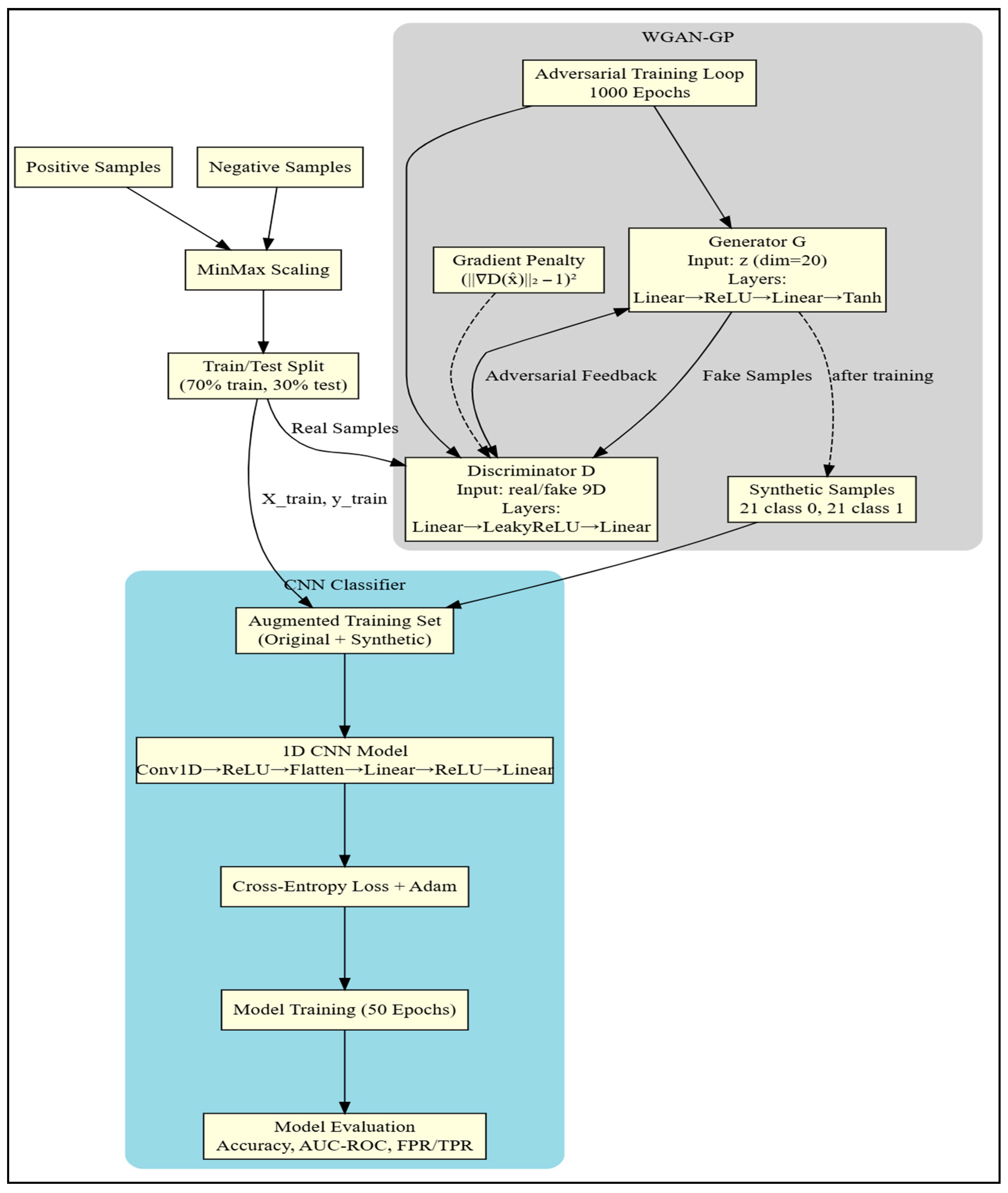
The model architecture combines a Wasserstein Generative Adversarial Network with Gradient Penalty (WGAN-GP) and a 1D Convolutional Neural Network (CNN) to improve mineral prospectivity classification. WGAN-GP consists of two networks: a generator (G) and a discriminator (D). The generator maps a 20-dimensional latent vector, sampled from a standard normal distribution to a 9-dimensional synthetic geochemical feature vector through fully connected layers with a final tanh activation (Table 1). The discriminator receives real or synthetic feature vectors and outputs a scalar score approximating the Wasserstein distance between real and generated data distributions. To stabilize training and satisfy the Lipschitz constraint, a gradient penalty term is added to the discriminator loss, computed from interpolated samples between real and synthetic data (Figure 6).
After adversarial training, the generator synthesizes additional negative samples, which are combined with the original data to create a balanced, augmented training set.
The CNN architecture is summarized in (Table 2). The nine input geochemical concentrations are first passed through a one-dimensional convolutional layer (Conv1D) that applies multiple filters across the input vector to extract localized features, enabling the model to distinguish geochemical patterns associated with prospective and non-prospective zones.
The ReLU activation introduces nonlinearity, allowing the network to capture complex relationships within the geochemical data. Extracted features are flattened and passed through fully connected layers to learn high-level representations, with the final layer producing classification outputs. The model is trained for 50 epochs using the Adam optimizer and cross-entropy loss. When training on WGAN-GP augmented data, this CNN shows improved classification performance and enhanced mineral prospectivity.

5.3. Machine Learning Results

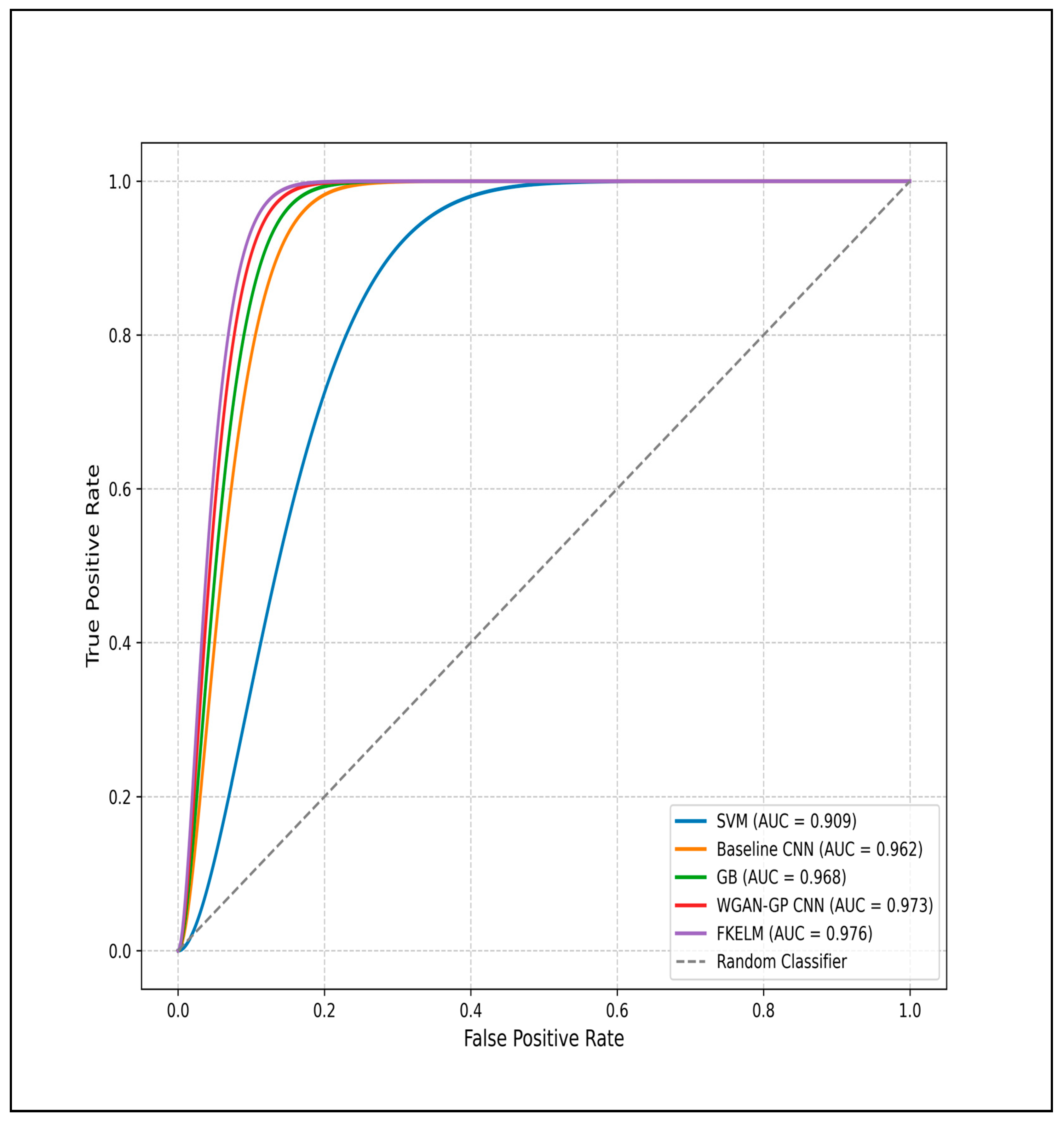
This study compares the performance of SVM, Gradient Boosting (GB), raw CNN, WGAN-GP CNN, and FKELM models. After 50 training epochs, model performance was evaluated using classification accuracy and ROC curves. The results show AUC values of 0.91 for SVM, 0.97 for GB, 0.96 for raw CNN, 0.97 for WGAN-GP CNN, and 0.98 for FKELM, indicating significant performance gains (Figure 7).
The SVM model achieves 90% training accuracy and 62% test accuracy. The raw CNN model reaches 93% and 85%, respectively. Gradient Boosting trained on the original data achieves 96% training and 90% test accuracy. After WGAN-GP data augmentation, training accuracy improves to 97% and test accuracy to 91%. FKELM achieves 100% training and 92% test accuracy (Table 3).
These results demonstrate that FKELM and WGAN-GP augmentation improve model generalization. By generating diverse and informative synthetic samples, WGAN-GP CNN and FKELM models effectively mitigate data scarcity and improve predictive performance.
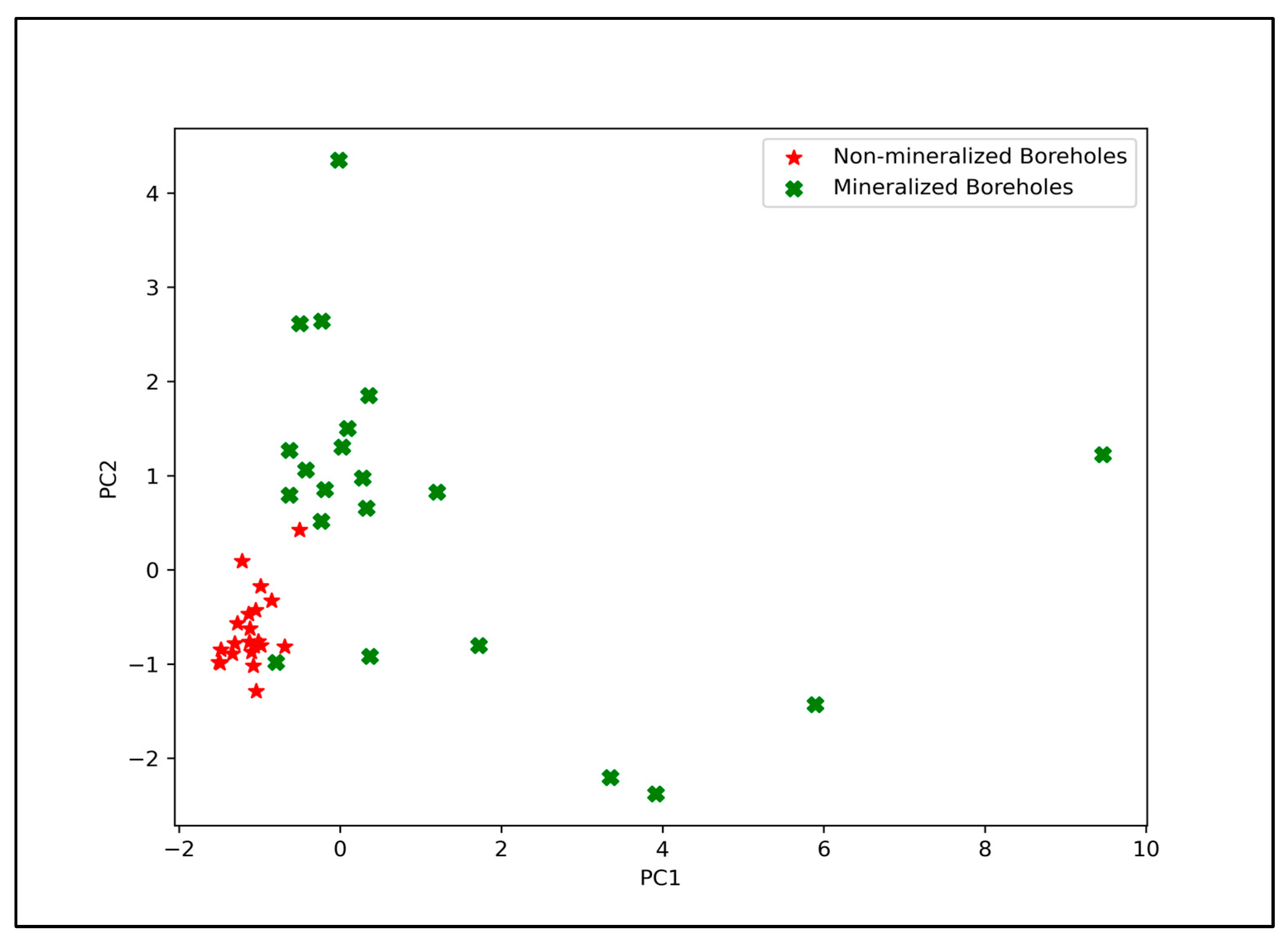
Earlier, feature scaling did not yield the expected results. Principal component analysis (PCA) was applied for dimensionality reduction.
PCA simplifies complex datasets by transforming variables into principal components (PCs). In this study, the variables were reduced to two principal components (PC1 and PC2), capturing 95% of the variance, before training the ML models. Figure 8 shows the patterns (PC1 vs. PC2), and Figure 9 shows the correlation of each variable with the principal components, revealing key geochemical relationships linked to mineralization.
The PCA-transformed data improved the performance of ML models, including SVM, GB, MLP, and Biased CNN, compared with previous results (Table 4). SVM and GB also showed higher AUC values (Figure 10). These findings confirm that PCA-based preprocessing enhances dimensionality reduction and improves model performance for mineral prospectivity mapping.
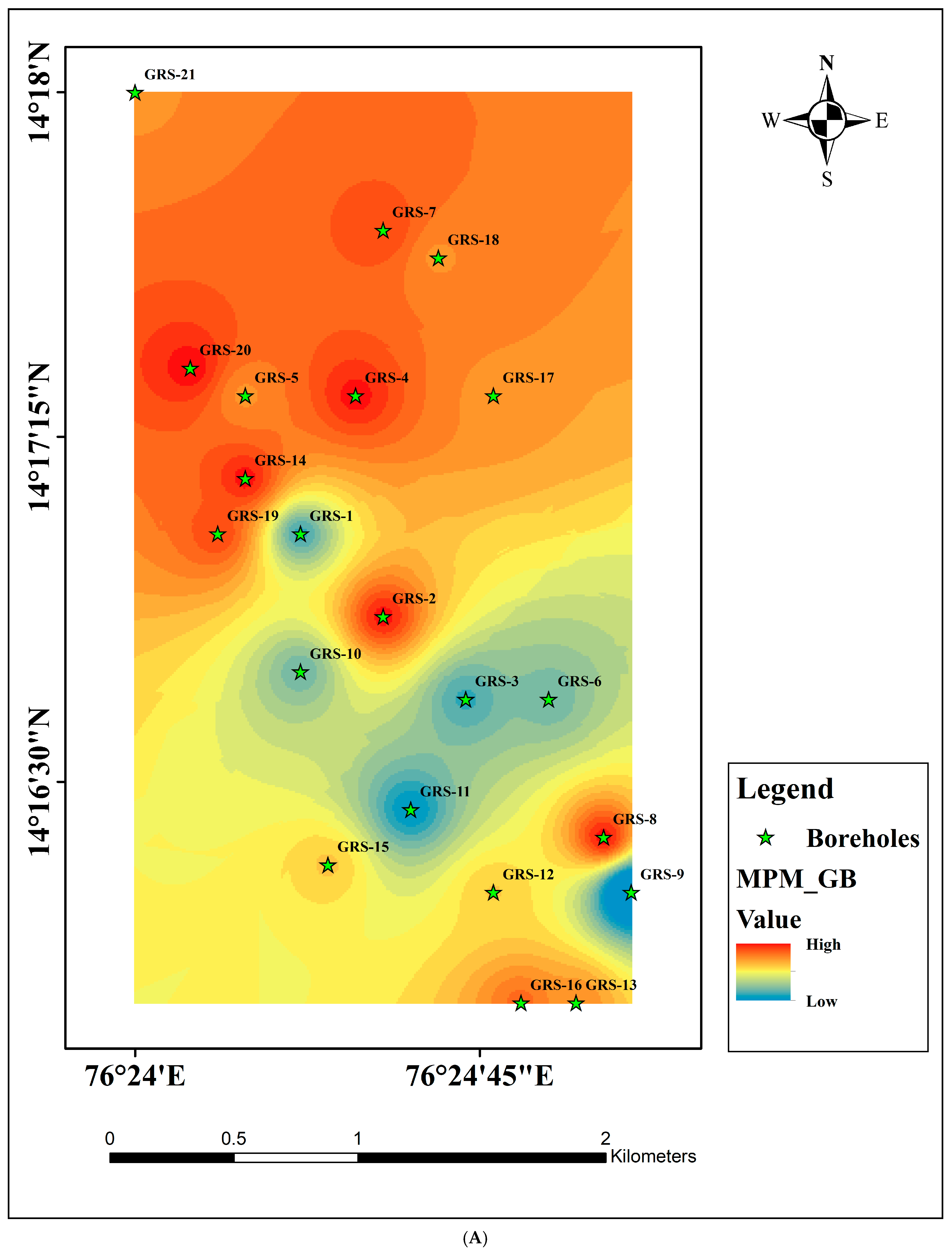
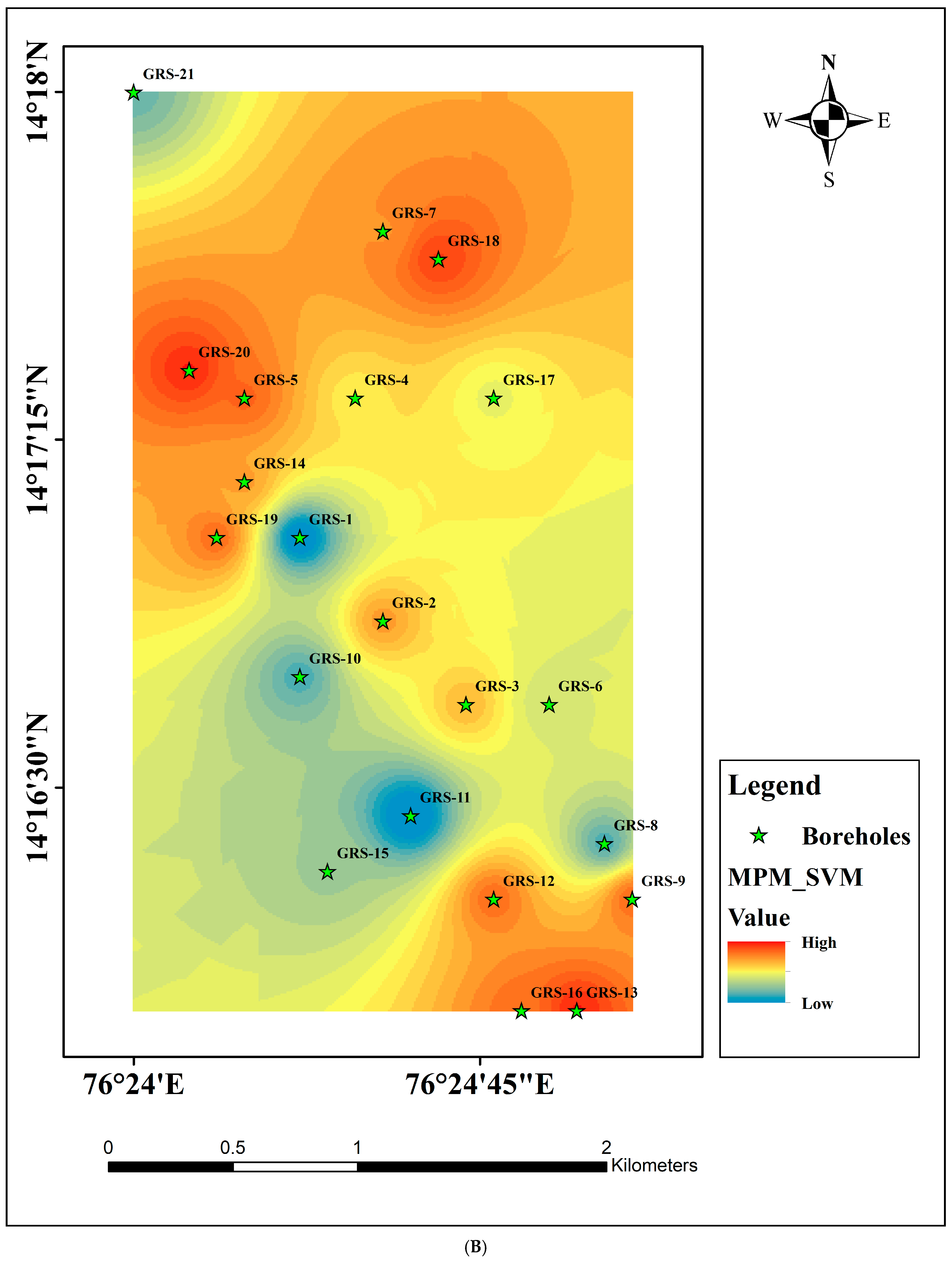
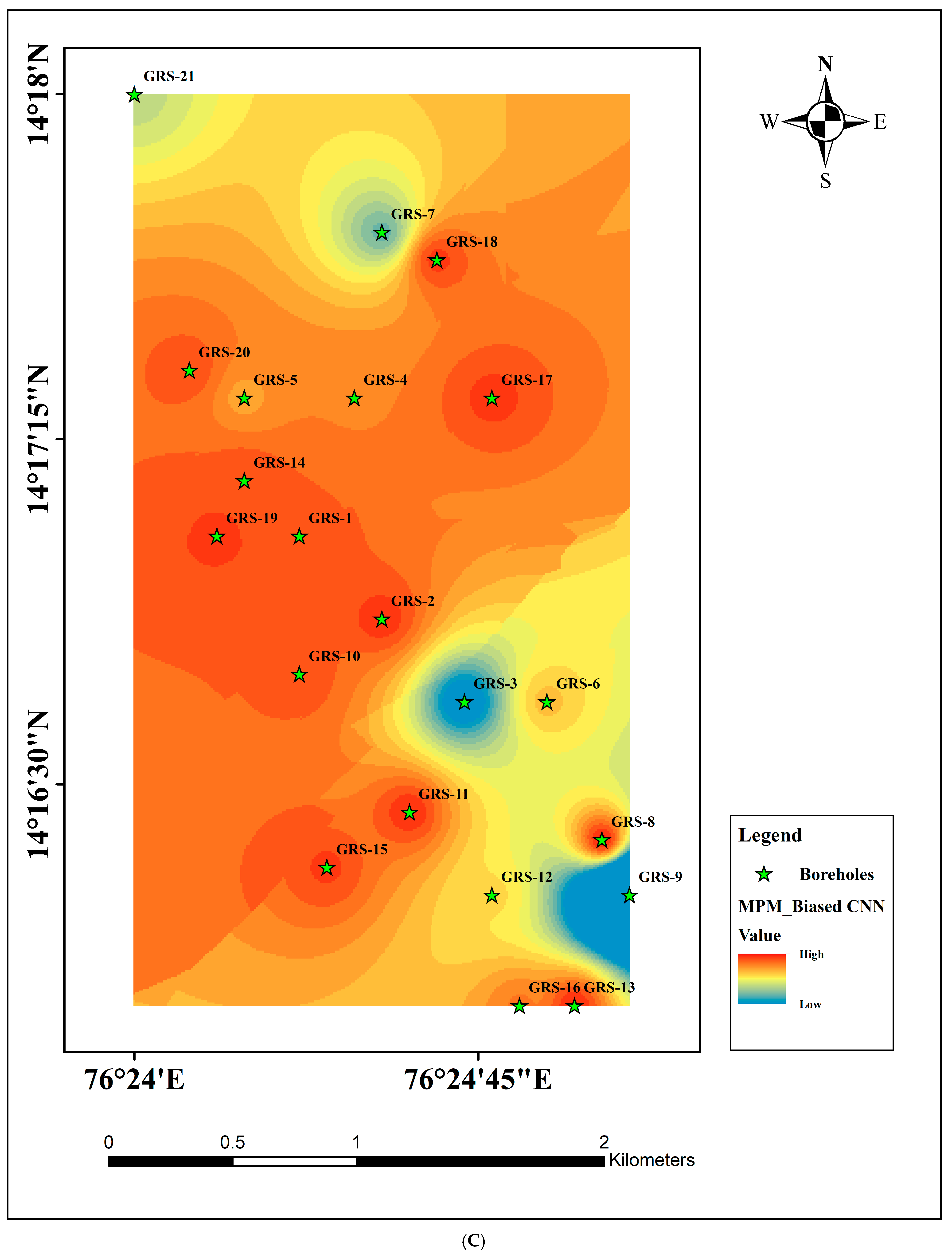
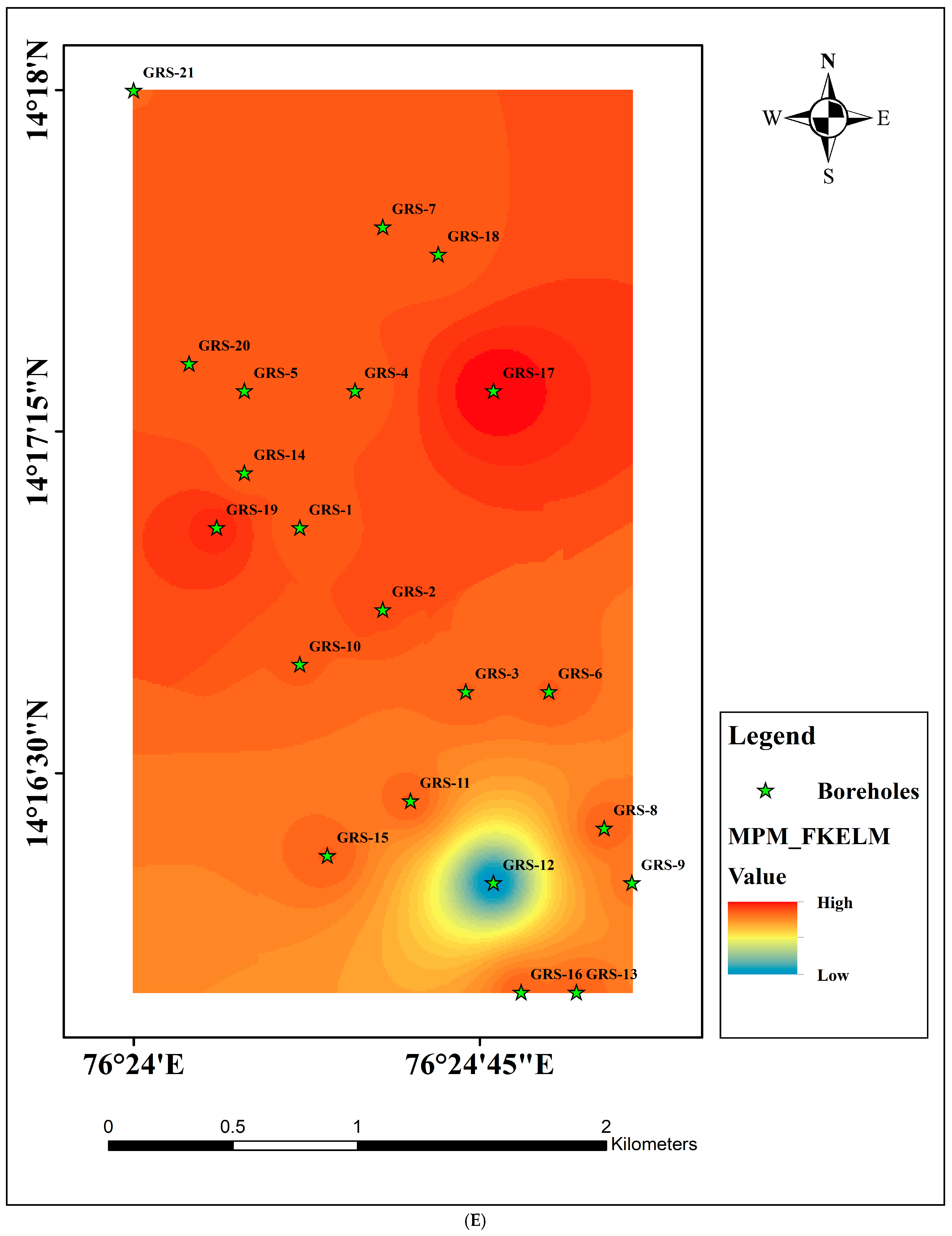
Based on the prediction results of all models, mineral prospectivity maps (MPMs) for the G.R. Halli South Block were generated (Figure 11A–E). MPMs effectively validate model performance, as high-potential regions identified by the models largely overlap with known ore locations. This confirms that GB can accurately map relationships between geochemical data and gold mineralization, showing strong feature extraction and predictive capabilities.
Because mineralization is a rare geological event, overly broad high-potential areas complicate exploration and conflict with regional geological understanding. In contrast, the MPM generated with WGAN-GP CNN displays more compact high-potential zones, aligning better with known geology and offering clearer exploration guidance. This improvement is attributed to the WGAN-GP CNN’s ability to introduce data variability and complexity, enabling the model to learn finer, more accurate feature representations and produce geologically realistic predictions.
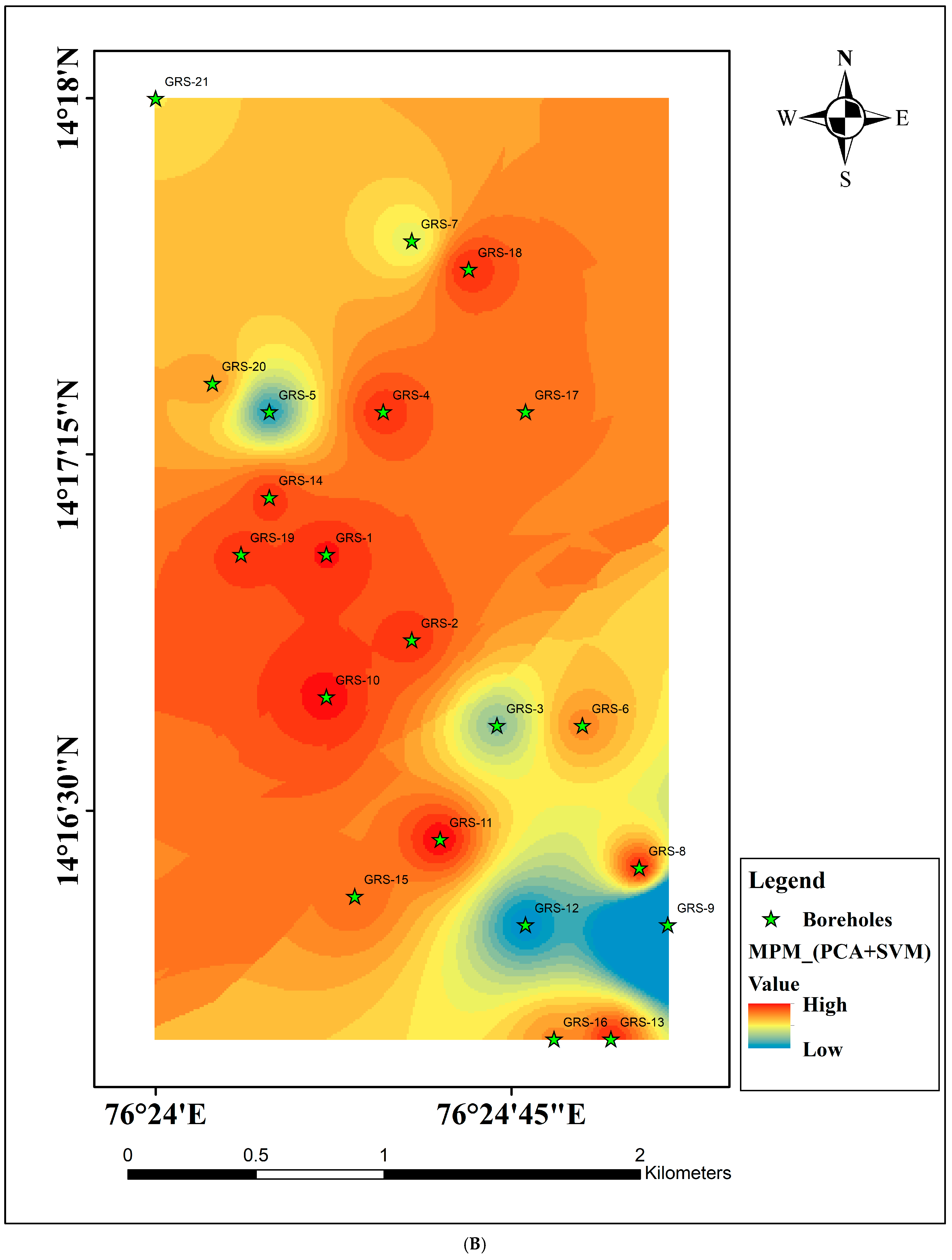
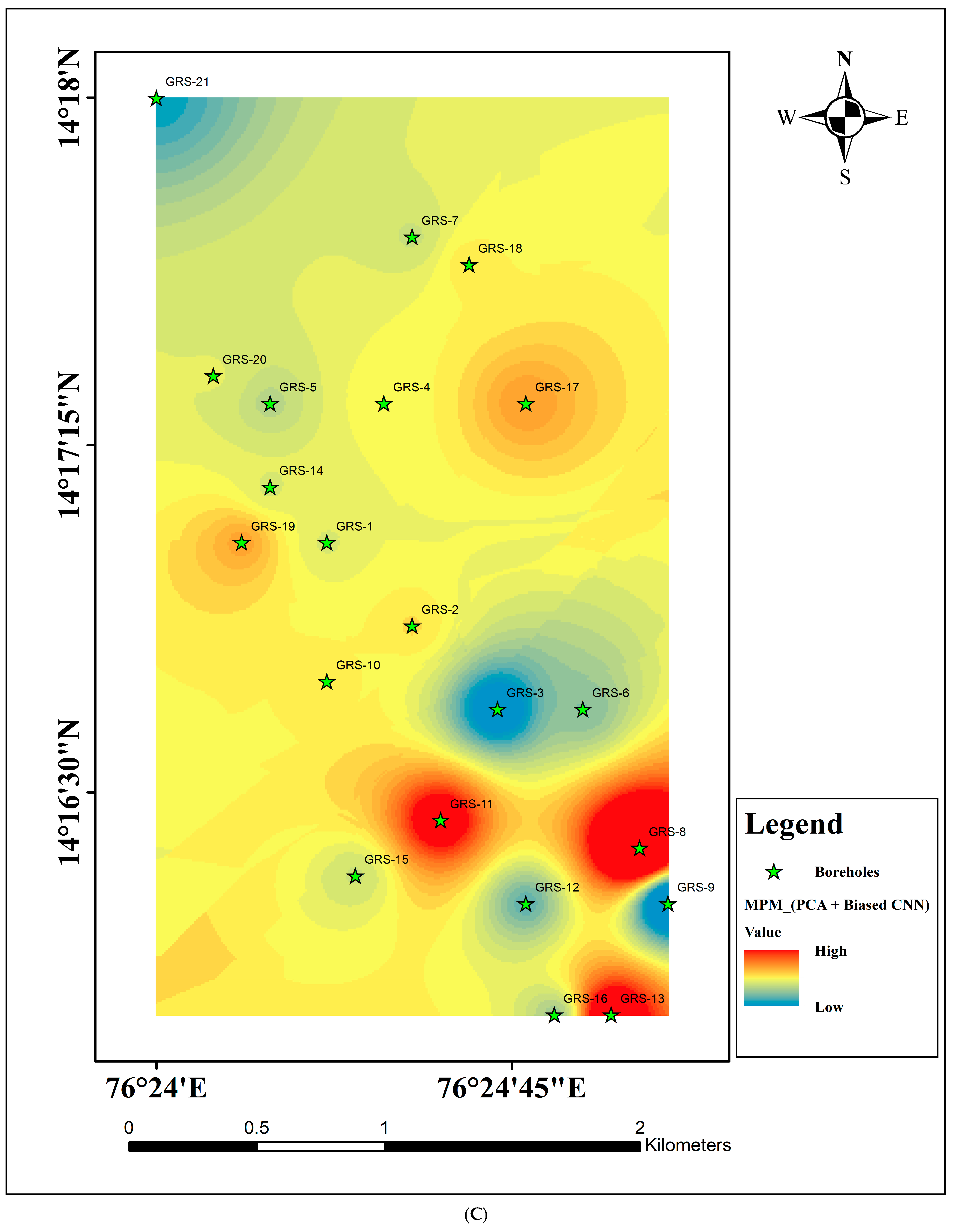
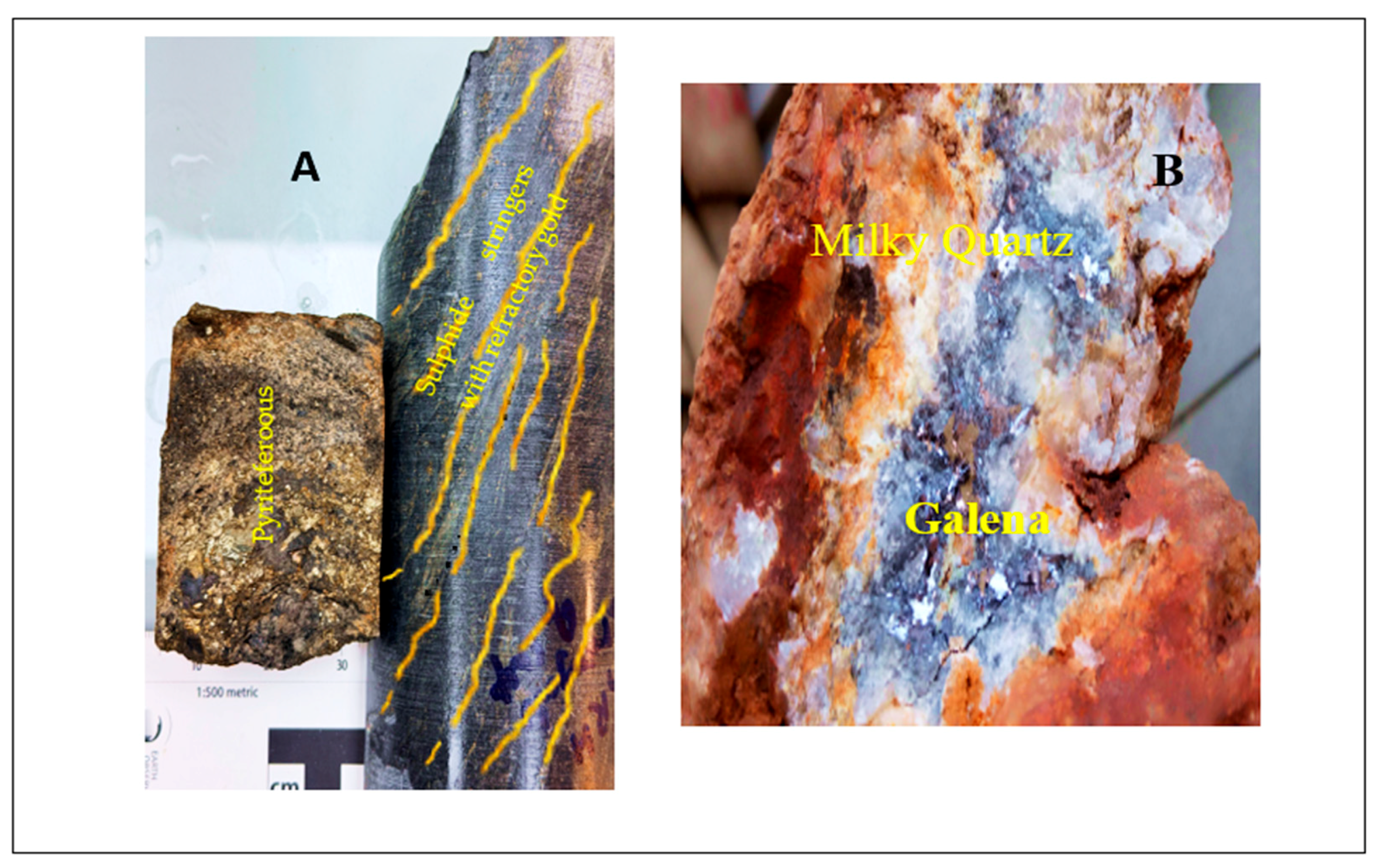
Machine learning models, including FKELM and WGAN-GP CNN, identified highly prospective auriferous zones, confirming their predictive reliability (Figure 11D,E; GRS-1, GRS-2, GRS-10, GRS-14). The PCA based mineral prospectivity maps are shown in (Figure 12A–D). To validate these results, borehole samples were analyzed for gold (Figure 13), yielding concentrations of up to 8 g/t Au, 1% As, 30 ppm Ag, and ~0.5% Pb.

6. Conclusions

This study proposes a hybrid framework for mineral prospectivity mapping (MPM) that integrates WGAN-GP CNN and Fuzzy Kernel Extreme Learning Machine (FKELM) models to address imbalanced datasets in mineral exploration. The experimental results show FKELM achieved the best performance (AUC = 0.976; test accuracy = 92%), as well as WGAN-GP CNN (AUC = 0.973; test accuracy = 91%), both outperforming conventional SVM, GB, and biased CNN models. Although PCA + GB (AUC = 0.971; test accuracy = 85%) shows slightly lower performance compared with AUC, it provides good results. Geochemical anomaly mapping reveals strong spatial correlations with gold and pathfinder elements (As, Sb, Zn, Pb, Ag, and Cu). The application of PCA to machine learning models such as SVM, GB, Biased CNN, and MLP improved results by 0.055, 0.003, and 0.01, respectively. These findings confirm that PCA-based pre-processing enhances dimensionality reduction and improves model performance in mineral prospectivity mapping, while PCA + GB should only be used as a relevant baseline for dimensionality reductions. The resulting prospectivity maps expose potential gold occurrences in barren zones in the G.R. Halli South Block, including areas with minimal wall rock alterations. Notably, the FKELM and WGAN-GP CNN models suggest high-prospectivity mineralized zones for green and brown field exploration. Future work should integrate geophysical datasets, test the framework on other mineral systems, and incorporate uncertainty quantification to further improve exploration targeting and decision-making.

Author Contributions

Funding acquisition, investigation, project administration and resources, writing, editing, and reviewing, compiling figures, and data conceptualization by P.V.S.R.; conceptualization, data curation, visualization, and writing of the original draft by V.S.M.; editing of the original draft by A.G. All authors have read and agreed to the published version of the manuscript.

Funding

This research was funded by the Department of Science and Technology-Science and Engineering Research Board (DST-SERB), Government of India.

Data Availability Statement

The datasets analyzed during the current study are available in the GitHub repository. Available online: https://github.com/Venkatasaimudili/MPM_Gold.git (accessed on 1 September 2025). The repository contains geochemical datasets (positive and negative borehole samples with elemental concentrations). Access to the original dataset may be considered by the corresponding author upon reasonable request.

Acknowledgments

We are very thankful to Prakash Kumar, CSIR-National Geophysical Research Institute, for providing all the facilities to carry out this work and for the kind permission to publish this paper. We thank Negi, Dean School of information Sciences UOH. The authors acknowledge ANRF-CRG, New Delhi, and Saleem Khan, Consultant Geologist for his valuable discussions.

Conflicts of Interest

The authors declare no conflicts of interest.

Code Availability Statement

Name of the code/library: Mineral prospectivity mapping framework. Hardware requirements: Standard environment with GPU support (min. 8 GB GPU memory recommended). Program language: Python (v3.8 or higher). Software required: TensorFlow/Keras, NumPy, Pandas, Scikit-learn, Matplotlib, ArcGIS (for spatial mapping). Program size: ~50 MB. A link to download the code is: {https://github.com/Venkatasaimudili/MPM_Gold.git}.

References

  1. Kong, Y.; Chen, G.; Liu, B.; Xie, M.; Yu, Z.; Li, C.; Wu, Y.; Gao, Y.; Zha, S.; Zhang, H.; et al. 3D mineral prospectivity mapping of Zaozigou gold deposit, west Qinling, China: Machine learning-based mineral prediction. Minerals 2022, 12, 1361. [Google Scholar] [CrossRef]
  2. Cracknell, M.J.; Reading, A.M. Geological mapping using remote sensing data: A comparison of five machine learning algorithms, their response to variations in the spatial distribution of training data and the use of explicit spatial information. Comput. Geosci. 2014, 63, 22–33. [Google Scholar] [CrossRef]
  3. Zhang, S.; Carranza, E.J.M.; Wei, H.; Xiao, K.; Yang, F.; Xiang, J.; Zhang, S.; Xu, Y. Data-driven mineral prospectivity mapping by joint application of unsupervised convolutional auto-encoder network and supervised convolutional neural network. Nat. Resour. Res. 2021, 30, 1011–1031. [Google Scholar] [CrossRef]
  4. Gong, J.; Li, Y.; Xie, M.; Kong, Y.; Tang, R.; Li, C.; Wu, Y.; Wu, Z. Mineral Prospectivity Mapping in Xiahe-Hezuo Area Based on Wasserstein Generative Adversarial Network with Gradient Penalty. Minerals 2025, 15, 184. [Google Scholar] [CrossRef]
  5. Ganivada, A.; Mukhtar, S. Type2 Fuzzy Kernel-Based Multi-layer Extreme Learning Machine. In 7th International Conference on Soft Computing: Theories and Applications; Springer: Singapore, 2023; pp. 601–609. [Google Scholar] [CrossRef]
  6. Boadi, B.; Raju, P.V.S.; Wemegah, D.D. Analysing multi-index overlay and fuzzy logic models for lode-gold prospectivity mapping in the Ahafo gold district–Southwestern Ghana. Ore Geol. Rev. 2022, 148, 105059. [Google Scholar] [CrossRef]
  7. Yang, S.; Tian, S. Extraction of alteration information from hyperspectral data based on kernel extreme learning machine. Remote Sens. 2024, 16, 3646. [Google Scholar] [CrossRef]
  8. Zuo, R.; Carranza, E.J.M. Support vector machine: A tool for mapping mineral prospectivity. Comput. Geosci. 2011, 37, 1967–1975. [Google Scholar] [CrossRef]
  9. Fan, M.; Xiao, K.; Sun, L.; Zhang, S.; Xu, Y. Automated hyperparameter optimization of gradient boosting decision tree approach for gold mineral prospectivity mapping in the Xiong’ershan area. Minerals 2022, 12, 1621. [Google Scholar] [CrossRef]
  10. Zhang, H.; Xie, M.; Dan, S.; Li, M.; Li, Y.; Yang, D.; Wang, Y. Optimization of Feature Selection in Mineral Prospectivity Using Ensemble Learning. Minerals 2024, 14, 970. [Google Scholar] [CrossRef]
  11. Yu, Z.; Cui, W. Robust hyperspectral image classification using generative adversarial networks. Inf. Sci. 2024, 666, 120452. [Google Scholar] [CrossRef]
  12. Qian, H.; Geng, Y.; Wang, H. Lithology identification based on ramified structure model using generative adversarial network for imbalanced data. Geoenergy Sci. Eng. 2024, 240, 213036. [Google Scholar] [CrossRef]
  13. Naqvi, S.M.; Divakar Rao, V.; Narain, H. The Protocontinental growth of the Indian Sheild and antiquity of its rift valleys. Precambrian Res. 1974, 1, 345–398. [Google Scholar] [CrossRef]
  14. Radhakrishna, B.P.; Naqvi, S.M. Precambrian continental crust of India and its evolution. J. Geol. 1986, 94, 145–166. [Google Scholar] [CrossRef]
  15. Foote, R.B. Notes on the geology of parts of Bellary and Ananthapur districts. Rec. Geol. Surv. India 1886, 19, 97–111. [Google Scholar]
  16. Naqvi, S.M. The oldest supracrustals of the Dharwar Craton. J. Geol. Soc. India 1981, 22, 458–469. [Google Scholar] [CrossRef]
  17. Swami Nath, J.; Ramakrishnan, M. Early Precambrian supracrustals of Southern Karnataka. Mem. Geol. Surv. India 1981, 112, 23–38. [Google Scholar]
  18. Divakar Rao, V.; Rama Rao, P. Granitic activity and crustal growth in the Indian Sheild. Precambrian Res. 1982, 16, 257–271. [Google Scholar] [CrossRef]
  19. Naqvi, S.M.; Rogers, J.J.W. (Eds.) Precambrian of South India. Mem. Geol. Soc. India 1983, 4, 1–575. [Google Scholar]
  20. Naqvi, S.M.; Rogers, J.J.W. Precambrian Geology of India. In Oxford Mono-Graphs on Geology and Geophysics; Oxford University Press: Oxford, UK, 1987; Volume 6. [Google Scholar]
  21. Radhakrishna, B.P. Archaean granite-greenstone terrane of South India Sheild. Mem. Geol. Soc. India 1983, 4, 1–46. [Google Scholar]
  22. Radhakrishna, B.P. Crustal evolution and Metallogeny- Evidence from the Indian Shield. J. Geol. Soc. India 1984, 25, 617–640. [Google Scholar] [CrossRef]
  23. Pichamuthu, C.S.; Srinivasan, R. The Dharwar Craton; Perspective Report Series 7; Indian National Science Academy: New Delhi, India, 1984. [Google Scholar]
  24. Rogers, J.J.W. Dharwar Craton and the assembly of Peninsular India. J. Geol. 1986, 94, 129–143. [Google Scholar] [CrossRef]
  25. Chadwick, B.; Vasudeva, V.; Swaminathan, J. Statigraphy and structure of late Archaean Dharwar volcanic and sedimentary rocks and their base- ments in a part of the Shimoga basin east of Badravathi, Karnataka. J. Geol. Soc. India 1988, 32, 1–19. [Google Scholar] [CrossRef]
  26. Chardon, D.; Choukroune, P.; Jayananda, M. Sinking of the Dharwar Basin (South India): Implications for Archaean tectonics. Precambrian Res. 1998, 91, 15–39. [Google Scholar] [CrossRef]
  27. Naha, K.; Srinivasan, R.; Jayaram, S. Structural evolution of the PeninsularGneiss—An Early Precambrian migmatitic complex from South India. Geol. Rundsch. 1990, 79, 99–109. [Google Scholar] [CrossRef]
  28. Ramakrishnan, M. Nuggihalli and Krishnarajpet belts, Early Precambrian supracrustals of southern Karnataka: India edn, Early Precambrian Supracrustals of Southern Karnataka, Geo! Surv. India Memo 1981, 112, 249–259. [Google Scholar]
  29. Swaminath, J.; Ramakrishnan, M.; Viswanatha, M.N. Dharwar stratigraphic model and Karnataka craton evolution. Rec. Geol. Surv. India 1976, 107, 149–175. [Google Scholar]
  30. Raju, P.V.S.; Babu EVSSK and Merkle, R.K.W. New Data on the mineralogy of chromite from the Nuggihalli Shist belt, Western Dharwar Craton, Karnataka, India: Petrogentic Implications. Acta Geol. Sin. (Engl. Ed.) 2011, 85, 107–115. [Google Scholar] [CrossRef]
  31. Raju, P.V.S. Petrography and geochemical behaviour of trace element, REE and precious metal signatures in sulphidic banded iron formation of C.S. Halli, Chitradurga Schist Belt, Dharwar Craton. J. Asian Earth Sci. 2009, 34, 663–673. [Google Scholar] [CrossRef]
  32. Raju, P.V.S.; Charan, S.N.; Subba Rao, D.V.; Uday Raj, B.; Naqvi, S.M. Nature of shear zone hosted epigenetic gold mineralisation in BIF of Chitradurga Schist Belt, Karnataka. J. Geol. Soc. India 2006, 68, 577–581. [Google Scholar]
  33. Khan, S.A. Final Report on Investigation for Gold in G. R. Halli South Block, Chitradurga Schist Belt. Geol. Surv. India Unpub. Prog. Rep. FS 1993, 1992, 1994–1995. [Google Scholar]
  34. Jayananda, M.; Santosh, M.; Aadhiseshan, K.R. Formation of Archean (3600–2500 Ma) continental crust in the Dharwar Craton, southern India. Earth-Sci. Rev. 2018, 181, 12–42. [Google Scholar]
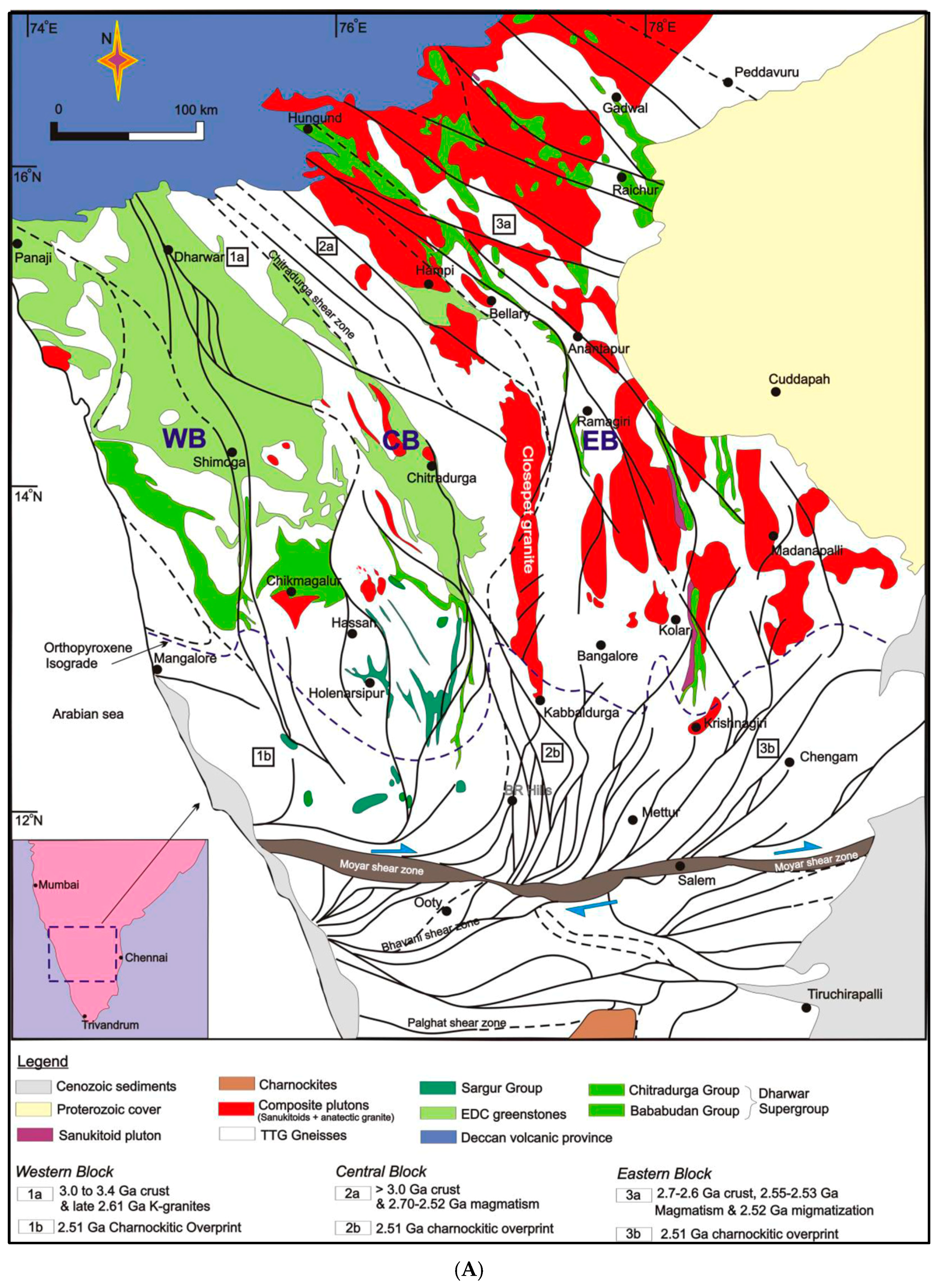
Figure 1. (A) Geological Map of the Dharwar Craton modified after [34]; there are three micro blocks (Western, Central and Eastern); (B) Borehole lithologies.
Minerals 15 01125 g001aMinerals 15 01125 g001b
Figure 2. Box diagram of the proposed hybrid mineral prospectivity mapping framework.
Minerals 15 01125 g002
Figure 3. Element concentration binary diagram.
Minerals 15 01125 g003
Figure 4. Element concentration map of gold (Au).
Minerals 15 01125 g004
Figure 5. (A) Study area map of G R Halli South block, and bore locations; (B) geological map of study area with boreholes.
Minerals 15 01125 g005aMinerals 15 01125 g005b
Figure 6. WGAN-GP structure diagram.
Minerals 15 01125 g006
Figure 7. The ROC-AUC of models (before PCA).
Minerals 15 01125 g007
Figure 8. Scatter plot between principal components.
Minerals 15 01125 g008
Figure 9. PCA loading diagram.
Minerals 15 01125 g009
Figure 10. The ROC-AUC of models (adding PCA).
Minerals 15 01125 g010
Figure 11. (A) Mineral prospectivity mapping using Gradient Boosting model; (B) mineral prospectivity mapping using Support Vector Machines; (C) mineral prospectivity mapping using Biased Convolution Neural Network; (D) mineral prospectivity mapping using Wasserstein Generative Adversarial Network with Gradient Penalty Convolutional Neural Network; (E) mineral prospectivity mapping using Fuzzy Kernel Extreme Learning Machines.
Minerals 15 01125 g011aMinerals 15 01125 g011bMinerals 15 01125 g011cMinerals 15 01125 g011dMinerals 15 01125 g011e
Figure 12. (A) Mineral prospectivity mapping using Gradient Boosting (adding PCA); (B) mineral prospectivity mapping using Support Vector Machines (adding PCA); (C) mineral prospectivity mapping using Biased Convolution Neural Network (adding PCA); (D) mineral prospectivity mapping using Multi-Layer Perceptron (adding PCA).
Minerals 15 01125 g012aMinerals 15 01125 g012bMinerals 15 01125 g012cMinerals 15 01125 g012d
Figure 13. Tested borehole sample after using Machine Learning models. (A) Borehole sample containing pyrite with refractory gold; (B) Milky quartz with native galena.
Minerals 15 01125 g013
Table 1. WGAN-GP network parameter table.
HyperparameterPositive SamplesNegative Samples
Initial learning rate0.00010.0001
Penalty coefficient10.010.0
Batch size88
Number of iterations (epochs)10001000
OptimizerAdamAdam
Latent Dimension20.020.0
Beta parameters(0.0, 0.9)(0.0, 0.9)
Table 2. CNN structure table.
Layer TypeParametersOutput ShapeActivation
Input1D vector (9 features)[Batch, 1, 9]-
Conv1DIn = 1, out = 32, kernel = 3[Batch, 32, 7]ReLU
Flatten-[Batch, 224]-
Linear (FC1)In = 224, out = 64[Batch, 64]ReLU
Linear (FC2)In = 64, out = 2[Batch, 2]-(Logits)
Table 3. Performance comparison of various classifiers (Before PCA).
ML ModelTrain AccuracyTest AccuracyAUC
SVM90%62%0.909
Raw CNN93%85%0.962
GB96%90%0.968
WGAN GP CNN97%91%0.973
FKELM100%92%0.976
Table 4. Performance comparison of various classifiers (Adding PCA).
ML ModelTrain AccuracyTest AccuracyAUC
PCA + Biased CNN86%92%0.952
PCA + MLP93%77%0.962
PCA + SVM97%92%0.964
PCA + GB97%85%0.971
WGAN GP CNN97%91%0.973
FKELM100%92%0.976
Disclaimer/Publisher’s Note: The statements, opinions and data contained in all publications are solely those of the individual author(s) and contributor(s) and not of MDPI and/or the editor(s). MDPI and/or the editor(s) disclaim responsibility for any injury to people or property resulting from any ideas, methods, instructions or products referred to in the content.