Comparing the Performance of Hydrocyclones and High-Frequency Screens in an Industrial Grinding Circuit: Part I—Size Separation Assessments

Abstract

Industrial ball milling circuits usually include hydrocyclones in a closed configuration to achieve a specified grinding size. Although hydrocyclones are relatively simple to operate, their classification performance is generally low, leading to significant fines recirculation within the circuit, consequently overgrinding the product. Conversely, high-frequency screening potentially shows a relatively higher separation efficiency, as the entrainment of fines to the coarse product is significantly reduced. The present work compares the performance of hydrocyclones—HC and high-frequency screens—HFS based on four surveys conducted in Nexa’s Vazante Zinc ore industrial grinding circuit in Vazante, Brazil, which processes zinc silicate ore. The comparisons included the partition of solids, water split, and particle size distributions. Whiten’s partition curve model was adopted to obtain the selected performance parameters through mass balancing the experimental data. The industrial surveys comprised three different size separation configurations, i.e., HC-Only, HFS-Only, and a combined HC-HFS setup. In all cases, the assessments consistently indicated higher separation performances with HFS compared to the HC operation. The final product associated with the HC+HFS configuration showed a narrower size distribution around the grinding size.

1. Introduction

Comminution circuits in industrial ore processing plants include equipment for size reduction and size separation, with the latter designed to obtain the stipulated product size [1]. Industrial grinding circuits in the mining industry are almost always configured in a closed configuration with hydrocyclones, where the underflow is circulated back to the mill, while the overflow is the circuit’s final product [2]. Although hydrocyclones are relatively simple to operate, their associated classification performance is generally low, resulting in a high recirculation of fines through the circuit, consequently overgrinding the product. Conversely, high-frequency screening “that uses frequencies of up to 3600 revolutions per minute (rpm) to separate down to 100 µm, as opposed to traditional vibrating screens that vibrate around 700–1200 rpm” [3], potentially shows a relatively higher separation efficiency, as fines in the coarse product are significantly reduced [4]. Examples can be found in the literature [4,5,6,7]. One of them, illustrated by Jankovic [5], demonstrates that replacing hydrocyclones with high-frequency fine screens resulted in a 13% increase in capacity and a 15% reduction in grinding energy. Improving the classification performance reduces the circuit’s energy consumption, as less energy is used for overgrinding [8,9,10]. Muketekelwa [11] observes that the degree of improvement is related to the type of hybrid configuration. For example, “a hybrid circuit with cyclone underflow reclassification exhibited a higher sharpness of separation value compared to a circuit with cyclone overflow reclassification”. More than that, in some cases changing the classification equipment from a size and density separation—as with a hydrocyclone—to a separation by size and shape only—a high frequency screen—generates not only an impact on the sharpness of separation but also an improvement of liberation properties for downstream processing [12]. In an ideal size separation operation, all particles coarser than a specific size would be forwarded to the coarse product, while particles finer than this size would flow to the fine product. However, in industrial separations, a fraction of fines is bypassed to the coarse product and a fraction of coarse particles is bypassed to the fine product.

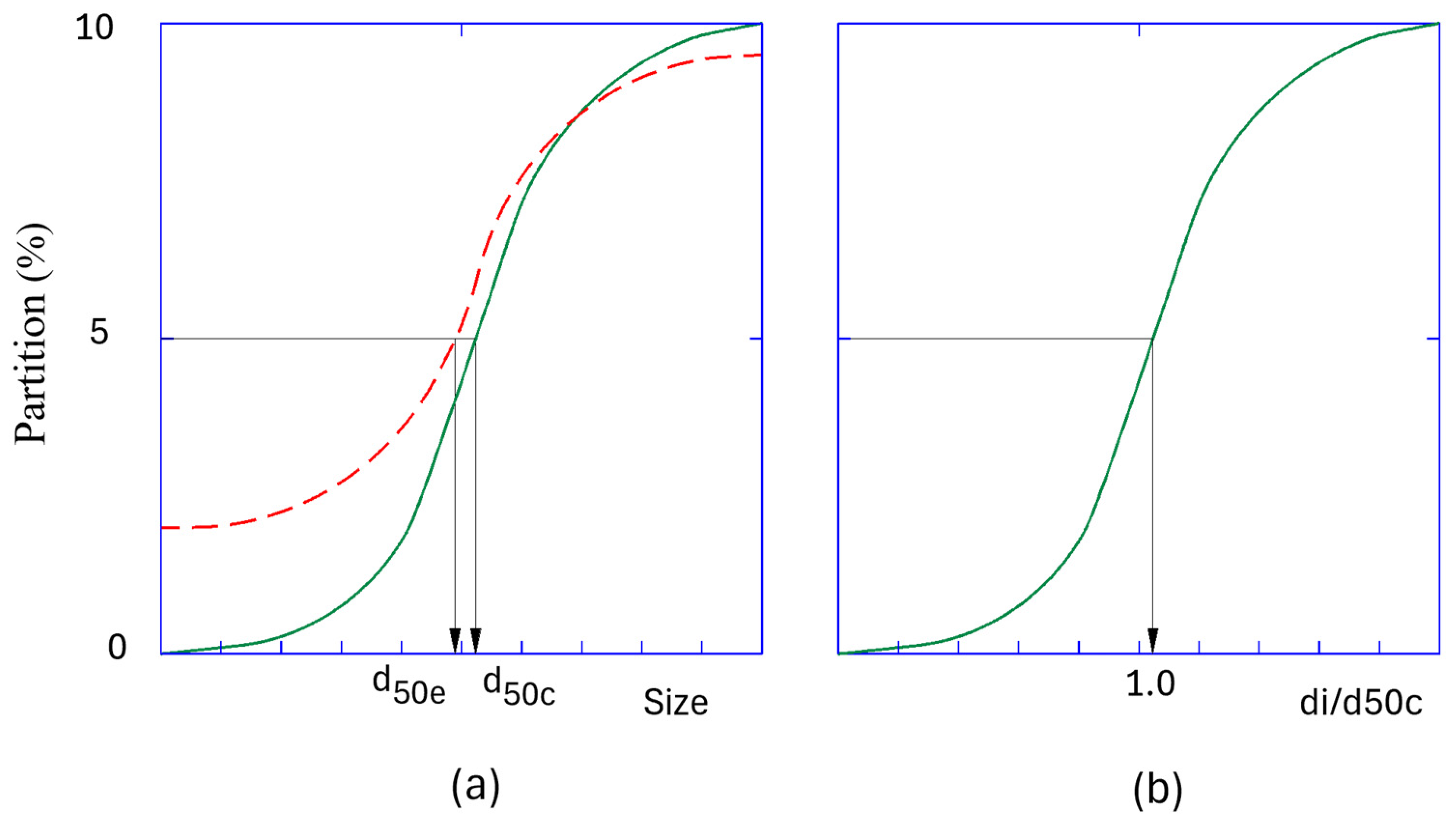
The partition curve is defined as the weight fraction of the feed reporting to the coarse or fine streams of the product [3]. Figure 1a shows an experimental partition curve obtained through experimental data. Three parameters are important for defining the characteristics of the curve. The first is a position parameter, referred to as the cut point d₅₀, defined as the size at which 50% of the particles in the feed report to the underflow. The second parameter is the sharpness of the cut, which corresponds to the slope of the central section of the partition curve. The third parameter is the bypass or short circuit of fines, which represents the amount of fine particles reporting to the underflow, graphically corresponding to the ordinate of the finest particle size plotted on the x-axis.

According to Kelsall [13] apud Wills [3] “solids of all sizes are entrained in the coarse product liquid, bypassing classification in direct proportion to the fraction of feed water reporting to the underflow”. Although this assumption is controversial [6], its relatively simple calculation is advantageous. By subtracting the entrained particles from the experimental partition, one obtains the corrected partition, which leads to the corrected partition curve, also shown in Figure 1a. This curve displays the d_50c parameter and accurately reflects the results of the true classification mechanisms.

A further representation of the partition is the standard or reduced curve proposed by Yoshioka and Hotta [14]. Accordingly, the abscissae are normalized by dividing each considered particle size by the d_50c parameter, as illustrated in Figure 1b. Therefore, a single graph compares different partition curves described only by the sharpness parameter. Lynch and Rao [15] and Nageswararao [16] assumed that reduced partition curves are independent of operating conditions and hydrocyclones sizes, with the latter in a relatively close range. At the same time, other authors [17,18,19] created specific equations to predict the sharpness parameter as a function of the hydrocyclones’ geometry and operating conditions.

Due to its central importance in modeling classification processes, the reduced partition curve has been described by different authors. Whiten parameterization [2] is presented in Equation (1), while Plitt’s [17] is shown in Equation (2), the latter being an adaptation of the Rosin–Rammler–Weibull equation.

$$y^{\prime }=\frac{{\mathrm{e}}^{\alpha xi}-1}{{\mathrm{e}}^{\alpha xi}+{\mathrm{e}}^{\alpha }-2}.$$

(1)

$${y^{\prime }=1-\mathrm{e}}^{{(-0.693xi}^{\mathrm{m}})} .$$

(2)

In Equations (1) and (2), the variable y’ represents the corrected partition, whereas xi indicates the ratio between the particle size and d_50c. The sharpness parameters are α in Whiten’s equation and m in Plitt’s equation. Based on the sharpness parameters α and m, Delboni Junior [20] created a criterion for assessing the performance of classification processes, as described in

Table 1. Separation performance as a function of the sharpness parameter.

Whiten Equation	Plitt Equation	Sharpness of Separation
α ≥ 4	m ≥ 2.9	Exceptional
3 ≤ α < 4	2.3 ≤ m < 2.9	Excellent
2 ≤ α < 3	1.6 ≤ m < 2.3	Good
1 ≤ α < 2	1 ≤ m < 1.6	Fair
α < 1	m < 1	Poor

.

Napier-Munn et al. [2] stipulated that the performance of the classification process was a function of the fraction of the feed liquid recovered by the coarse product, i.e., liquid split, as listed in

Table 2. Separation performance as a function of the liquid split.

Water Split to Coarse Product—WS (%)	Quality of Separation
WS ≥ 50	Very poor
40 ≤ WS < 50	Poor
30 ≤ WS < 40	Fair
20 ≤ WS < 30	Good
10 ≤ WS < 20	Excellent
< 10	Exceptional

.

1.1. Objective

The main objective of this work was to assess and compare the performances of hydrocyclones (HCs) and high-frequency screens (HFSs) installed in Nexa’s Vazante grinding circuit, a willemite (Zn₂SiO₄) mineral processing plant. The comparisons included the partition of solids, water split, and particle size distributions.

1.2. Vazante Industrial Mineral Processing Plant

Nexa’s Vazante mineral beneficiation process was designed to concentrate willemite (Zn₂SiO₄). The Vazante industrial circuit comprises multi-staged crushing, grinding, flotation, zinc concentrate thickening and filtering, and the filtering and stacking of tailings. The crushing and grinding stages are conducted in two parallel lines referred to as C and W [21,22,23,24,25]. However, the present work focuses only on the C grinding circuit.

Grinding circuit C includes two crushing stages equipped with a primary jaw crusher and a secondary cone crushing, resulting in a product with an average P₈₀ of 6.7 mm. The crushed product is stocked in conical piles, from which the reclaimed flow is conveyed to a dedicated grinding circuit. This circuit features a single ball mill operating in a closed configuration with a combination of high-frequency screens and hydrocyclones.

The product from the C grinding circuit is subsequently pumped to the flotation circuit, where the zinc concentrate is obtained. This concentrate undergoes thickening and filtering before being transported to Nexa’s Três Marias smelter. The flotation tailings are filtered and then stored in piles for disposal.

It is possible to observe a difference in recovery in the different particle size fractions present in the Vazante flotation feed [22,26]. The lowest recovery happens for the size fractions of +0.212 mm (27.7%) and +0.150 mm (48.9%). Intermediate ones occur for the sizes of +0.106 mm (81.5%) and passing 0.037 mm (83.5%), while the best recoveries happen of the sizes +0.053 mm (89.7%) and +0.037 (90.4%). Considering this point, a reduction in the coarse fraction that feeds the flotation, even with an increase in fines, can lead to a higher recovery.

2. Materials and Methods

2.1. Method

Two comprehensive survey campaigns were conducted on the C grinding circuit of the Vazante industrial plant on 7 April 2022, and 11 May 2023. Each campaign involved two surveys: the first with the combined operation of both HFSs and HCs, referred to as HFS+HC, or the hybrid configuration, and the second with HCs only, referred to as HC-Only. Due to piping and operational limitations in the industrial installations, surveys with HFS-Only were not carried out.

The adopted method included sampling individual streams around the circuit for their corresponding configuration, obtaining detailed data and information from the dedicated process information management system (PIMS), and measuring the vortex and apex of the hydrocyclones. The collected samples were processed in the Vazante Process Laboratory (VPL) to determine their respective solids concentration and size distributions. The mass balancing of experimental data was performed using JKSimMet 6.2 software.

2.2. Survey Campaigns

Figure 2 shows the C grinding circuit flow sheet, configured with a combination of HFSs and HCs. The sampling points are indicated on the same flow sheet. The mill discharge is pumped into the HC feed, whose underflow circulates back to the mill feed, while the combined overflow is pumped into the HFS feed. The HFS oversize also circulates back to the mill feed, while the undersize is the grinding circuit product.

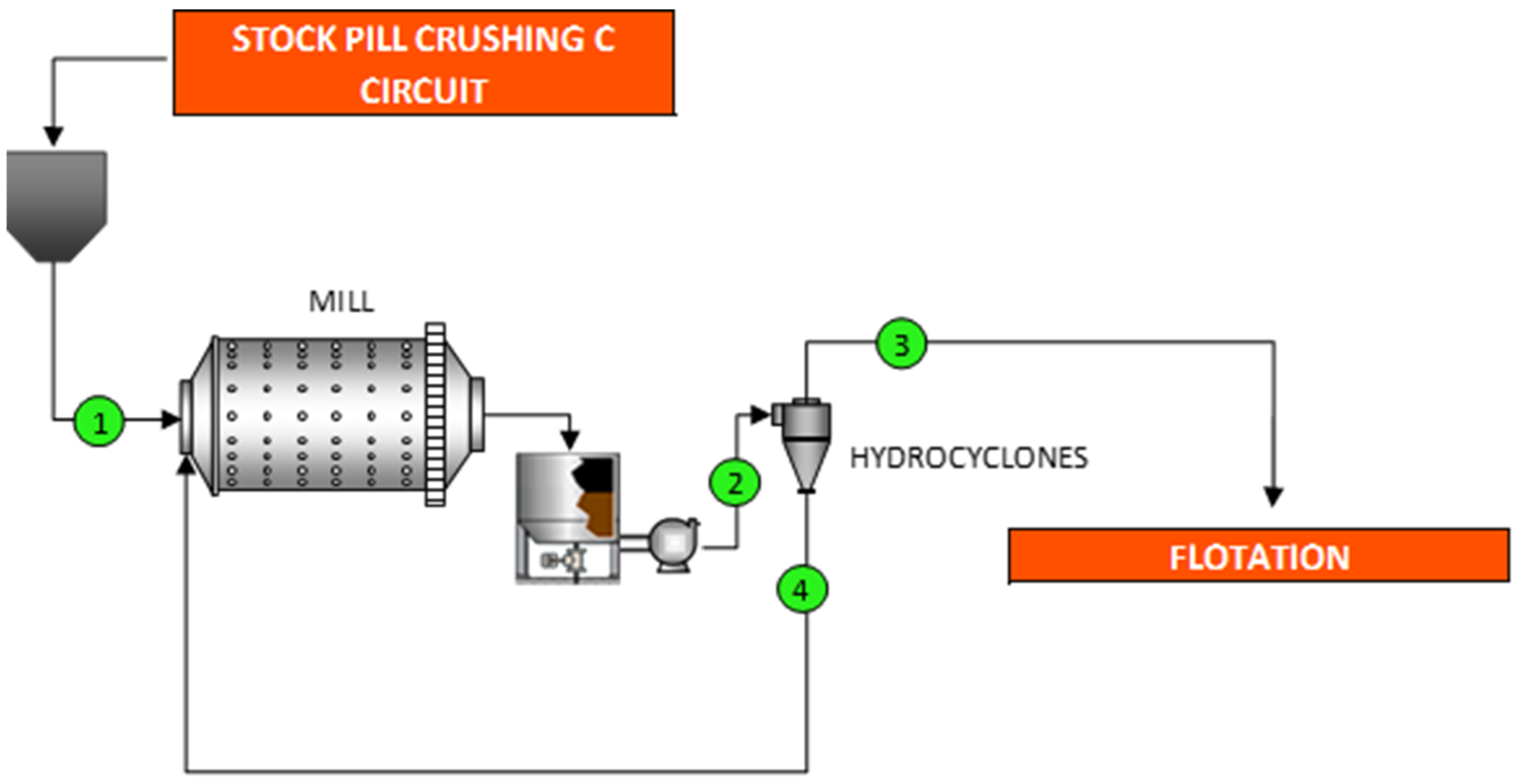
Figure 3 shows the C grinding circuit flow sheet according to the HC-Only configuration, including the four sampling points accessed in this work. In this configuration, the mill discharge is pumped into the HC feed, whose underflow circulates back to the mill feed, while the overflow is the grinding circuit product.

The main characteristics of the equipment installed in Circuit C are listed in

Table A1. Equipment characteristics—grinding circuit C.

Equipment	Unit	Circuit C
Ball Mill
Diameter—inside shell	m	2.9
Length—inside shell	m	11.0
Speed	% critical	75
Ball charge	%	25
Motor	kW	1300
Hydrocyclones
Diameter	mm	381
Vortex	mm	165
Apex	mm	95
Operating pressure	kPa	50
Units in normal operation	-	1
High-Frequency Screens
Width	mm	1770
Length	mm	5300
Aperture	mm	0.15
Frequency	Hz	1800
Units in normal operation	-	1

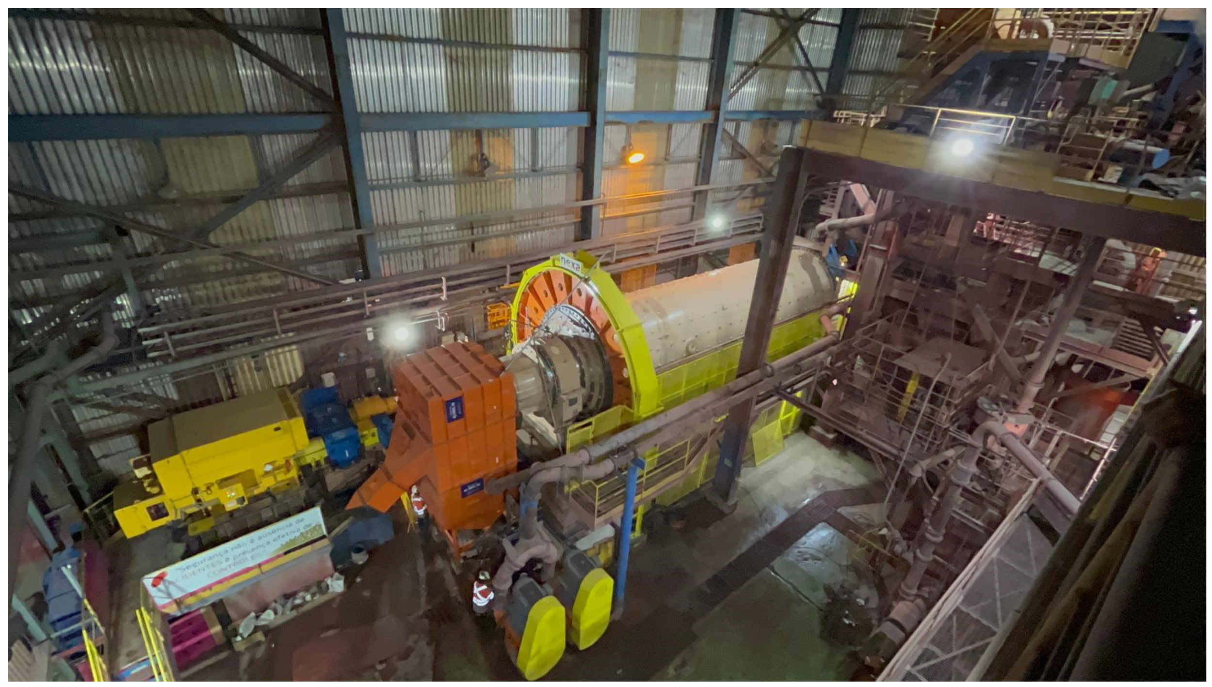
of Appendix A. Figure 4 shows a photograph of the industrial installations of the C grinding circuit.

2.3. Sample Processing

The collected pulp samples were weighed, filtered, dried in an oven, and weighed again in the VPL to determine the concentration of solids by weight. Circuit fresh feed samples followed the same procedure for calculating their respective moisture. Dry samples were split and wet sieved using laboratory sieves with the following sizes: 12.5 mm, 9.52 mm, 6.35 mm, 3.35 mm, 2.36 mm, 1.18 mm, 0.850 mm, 0.600 mm, 0.350 mm, 0.210 mm, 0.149 mm, 0.105 mm, 0.074 mm, 0.053 mm, 0.044 mm, 0.037 mm, and 0.020 mm. We used a vibrating suspended sieving machine with a capacity of up to ten 8 × 2 sieves. It is important to highlight that, in the first sampling campaigns, the 0.020 mm sieve was not used; however, in the last sampling, it was included to provide extended particle size distributions.

2.4. Mass Balance and Plotting the Partition Curve

The mass balancing of the experimental data was carried out for the different size separation devices, i.e., HC and/or HFS. For the HC, this process was based on the concentration of solids and the size distributions of the HC feed, underflow, and overflow. For the HFS, the feed, oversize, and undersize flows were mass-balanced in terms of solid concentration and size distributions. Detailed experimental data from the sampling and the corresponding mass balancing results are presented in

Table A2. Experimental and mass-balanced data, HFS+HC configuration—Campaign 1: (a) HC data; (b) HFS data.

(a)
Variable	Grinding Circuit Feed	HFS+HC Configuration—HC Data
		Experimental			Balanced
	Experimental	Feed	Underflow	Overflow	Feed	Underflow	Overflow
Solids (%)	96	50.8	80.3	32	52.7	74.9	29.8
Size (mm)	Accumulated Percent Passing
12.5	100	100	100	100	100	100	100
9.52	100	100	100	100	100	100	100
6.3	84.2	99.6	99	100	100	100	100
3.35	56.8	99.3	97.2	100	99.3	98.5	100
2	38.7	98.7	95	100	98.7	97.3	100
1.18	27	97.2	92.1	100	97.2	94.2	100
0.298	9	76.3	58.4	92.6	76.4	57.5	93.9
0.21	7.1	59.4	38.1	83.3	59.4	35.8	81.4
0.149	5.5	43.2	21.8	71.4	43.2	19.4	65.3
0.105	3.8	29	11.6	57.9	35	13	55.5
0.074	3.4	22.4	7.5	49.7	28.3	8.9	46.5
0.053	3.2	18.4	5	43.6	24.4	6.9	40.7
0.037	3	15.8	3.8	38.4	21.8	5.8	36.6
(b)
Variable	Grinding Circuit Feed	HFS+HC Configuration—HFS Data
		Experimental			Balanced
	Experimental	Feed	Oversize	Undersize	Feed	Oversize	Undersize
Solids (%)	96	31.9	80.6	33.2	37.5	72.9	30.3
Size (mm)	Accumulated Percent Passing
12.5	100	100	100	100	100	100	100
9.52	100	100	100	100	100	100	100
6.3	84.2	100	100	100	100	100	100
3.35	56.8	100	100	100	100	100	100
2	38.7	99.9	100	100	100	100	100
1.18	27	99.5	99.7	100	100	100	100
0.298	9	92.6	80.8	99.9	93.9	81.5	100
0.21	7.1	83.3	46.4	98.7	81.4	46.6	98.6
0.149	5.5	71.4	22.9	91.9	65.3	20.4	87.4
0.105	3.8	57.9	12.8	75.1	55.5	14.1	75.9
0.074	3.4	49.7	9.7	65.7	46.5	10.9	64
0.053	3.2	43.6	8	57.4	40.7	9.3	56.2
0.037	3	38.4	6.6	51.1	36.6	8.3	50.6

,

Table A3. Experimental and mass-balanced data, HC-Only configuration—Campaign 1.

Variable	Grinding Circuit Feed	HC-Only Configuration
		Experimental			Balanced
	Experimental	Feed	Underflow	Overflow	Feed	Underflow	Overflow
Solids (%)	96	60.5	84.3	32	60.5	84.1	31.1
Size (mm)	Accumulated Percent Passing
12.5	100	100	100	100	100	100	100
9.52	100	100	100	100	100	100	100
6.3	89.4	98.7	94.7	100	100	100	100
3.35	61.7	97.9	92.9	100	97.9	97.3	100
2	41.6	96.2	91.1	100	96.2	95.1	100
1.18	27.7	93.1	87.3	100	93.1	91.1	100
0.298	8.6	69.2	57.4	98.2	69.2	60.5	98.5
0.21	6.2	53.9	42.5	93.4	53.9	42.2	93.5
0.149	5.4	39.5	24.7	84.6	39.5	26.4	83.8
0.105	4.5	22.6	12.7	72.4	28	15.2	71.1
0.074	4	21.1	8.1	66	22	10.2	61.8
0.053	3.7	13.7	5.7	58.5	17.7	7.2	53.3
0.037	3.4	11.1	3.9	51.2	15.1	5.6	47.3

,

Table A4. Experimental and mass-balanced data, HFS+HC configuration—Campaign 2: (a) HC data; (b) HFS data.

(a)
Variable	Grinding Circuit Feed	HFS+HC Configuration—HC Data
		Experimental			Balanced
	Experimental	Feed	Underflow	Overflow	Feed	Underflow	Overflow
Solids (%)	96	80.3	41.9	59.1	82.8	39.3	59.1
Size (mm)	Accumulated Percent Passing
12.5	100	100	100	100	100	100	100
9.52	98.1	100	100	100	100	100	100
6.3	79.7	100	100	100	100	100	100
3.35	44.7	100	100	100	100	100	100
2.36	27.5	100	100	100	100	100	100
1.18	17.6	97.1	93.6	100	97.1	95.5	100
0.85	13.7	94.8	89.6	100	94.8	91.8	100
0.6	9.4	84.3	77.1	100	84.3	75.5	99.8
0.35	8	76.8	63.6	96	76.4	63.6	98.9
0.212	6.8	59.6	45	86	59.6	41.7	91.2
0.15	6	48.9	33.1	78	48.9	30	82.2
0.106	4.9	35.3	20.3	67	35.3	17.5	66.4
0.075	4.9	26.2	10.2	56.2	28.4	12.4	56.6
0.053	3.8	21.8	7.1	50.2	23.8	9.4	48.9
0.045	3.2	16.7	4.9	41.6	21	7.9	44.1
0.037	3.2	14.9	4.1	40.3	18.5	6.6	39.5
0.02	2.8	12.6	3.6	33.6	15.5	5.3	33.4
(b)
Variable	Grinding Circuit Feed	HFS+HC Configuration—HFS Data
		Experimental			Balanced
	Experimental	Feed	Oversize	Undersize	Feed	Oversize	Undersize
Solids (%)	96	41.9	71.3	37.7	39.3	83.7	35.9
Size (mm)	Accumulated Percent Passing
12.5	100	100	100	100	100	100	100
9.52	98.1	100	100	100	100	100	100
6.3	79.7	100	100	100	100	100	100
3.35	44.7	100	100	100	100	100	100
2.36	27.5	100	100	100	100	100	100
1.18	17.6	100	100	100	100	100	100
0.85	13.7	100	100	100	100	100	100
0.6	9.4	100	97.9	100	99.8	98.8	100
0.35	8	96	91.8	100	98.9	92.7	100
0.212	6.8	86	53.7	97.7	91.2	54.3	97.8
0.15	6	78	33	92.2	82.2	32.7	91.1
0.106	4.9	67	17	79.5	66.4	16.1	75.5
0.075	4.9	56.2	13	66.3	56.6	10.7	64.9
0.053	3.8	50.2	9.5	59.8	48.9	8.1	56.3
0.045	3.2	41.6	8.5	49.5	44.1	6.8	50.8
0.037	3.2	40.3	8.2	47.8	39.5	5.8	45.6
0.02	2.8	33.6	6.9	40.4	33.4	4.6	38.6

and

Table A5. Experimental and mass-balanced data, HC-Only configuration—Campaign 2.

Variable	Grinding Circuit Feed	HC-Only Configuration
		Experimental			Balanced
	Experimental	Feed	Underflow	Overflow	Feed	Underflow	Overflow
Solids (%)	97.3	53.2	72.8	39.9	53.2	74.4	37.2
Size (mm)	Accumulated Percent Passing
12.5	100	100	100	100	100	100	100
9.52	98.1	100	100	100	100	100	100
6.3	79.7	100	100	100	100	100	100
3.35	44.7	100	100	100	100	100	100
2.36	27.5	100	100	100	100	100	100
1.18	17.6	98.9	96.2	100	98.9	98.2	100
0.85	13.7	97.9	94.1	100	97.9	96.5	100
0.6	9.4	91.6	83	100	91.6	86.2	99.8
0.35	8	83.6	70.9	97.7	83.4	73.3	98.4
0.212	6.8	69.7	52.2	90.3	69.7	54.7	92.3
0.15	6	59.4	39.7	82.6	59.4	42.5	84.8
0.106	4.9	44.3	23.5	71.2	44.3	27.1	70.1
0.075	4.9	34.1	13.5	60.8	34.2	18.3	58.1
0.053	3.8	28.5	9.4	53.2	28.2	13.8	49.9
0.045	3.2	23.3	7	44.4	25.3	11.8	45.5
0.037	3.2	22.6	6.8	43	22.6	10.1	41.5
0.02	2.8	19.5	5.6	36.7	19.6	8.4	36.3

in Appendix B. The resulting mass-balanced data were used to calculate both experimental and corrected partitions associated with each one of the two campaigns, as detailed in

Table A6. Partition data—Campaign 1.

Size	HFS+HC									HC-Only
	Combined HFS+HC			HFS+HC—HC-Only			HFS+HC—HFS-Only
	Partition		di/d50c	Partition		di/d50c	Partition		di/d50c	Partition		di/d50c
(mm)	Exper	Corr		Exper	Corr		Exper	Corr		Exper	Corr
2	100	100	17.5	100	100	11.8	100	100	13.9	100	100	29.9
1.18	100	100	10.4	100	100	6.9	100	100	8.2	100	100	17.6
0.298	99.9	99.9	2.6	95.2	94.6	3	99.8	99.8	2.1	98.6	98.2	4.4
0.21	96.6	95.8	1.8	84.8	82.9	1.8	92.6	92	1.5	92.5	90.3	3.1
0.149	79.7	75.1	1.3	62	57.3	1.2	53.8	50.1	1	84.6	80.2	2.2
0.105	52.2	41.3	0.92	50.3	44.1	0.88	21.5	15.3	0.73	75.1	67.9	1.57
0.074	34.2	19.2	0.65	37.8	30.1	0.62	11.7	4.7	0.51	64.3	54.1	1.1
0.053	26.3	9.5	0.46	29.9	21.2	0.44	9.2	1.9	0.37	54.9	42	0.79
0.037	22.7	5.2	0.32	24.3	15	0.35	8.2	0.9	0.26	47	31.7	0.55

and

Table A7. Partition data—Campaign 2.

Size	HFS+HC									HC-Only
	Combined HFS+HC			HFS+HC—HC-Only			HFS+HC—HFS-Only
	Partition		di/d50c	Partition		di/d50c	Partition		di/d50c	Partition		di/d50c
(mm)	Exper	Corr		Exper	Corr		Exper	Corr		Exper	Corr
1.18	100	100	11.7	100	100	10.7	100	100	6.9	100	100	11.2
0.85	100	100	8.4	100	100	7.7	100	100	4.9	100	100	8.1
0.6	100	100	5.9	99.4	99.2	5.5	100	100	3.5	98.5	98	5.7
0.35	100	100	3.5	95.6	94.6	3.2	99.6	99.5	2	93.6	91.6	3.3
0.212	98.6	98.2	2.1	83.5	79.6	1.9	76.1	75.6	1.2	82.3	76.8	2
0.15	88	84.3	1.5	69.4	62.1	1.4	36.7	35.4	0.87	70.7	61.7	1.4
0.106	64.5	53.4	1	58.1	48.2	1	17.3	15.6	0.62	61.1	49.2	1
0.075	45.5	28.5	0.74	48.1	35.8	0.68	8.5	6.7	0.44	52.5	38	0.71
0.053	34.8	14.5	0.52	40.4	24	0.48	5.2	3.4	0.31	45.4	28.7	0.5
0.045	30.6	9	0.45	35.4	20	0.41	4	2.1	0.26	40.6	22.4	0.43
0.037	29	6.9	0.37	33.2	17.3	0.34	3.6	1.7	0.22	38.4	19.5	0.35
0.02	26.9	4.1	0.2	28.1	11	0.18	2.8	0.9	0.12	33.2	12.7	0.19

in Appendix C. The feed water fraction to the underflow and the parameters d_50c and α obtained from White’s equation to parameterize the different partition curves were used to assess and compare individual classification performances. Grinding circuit product size distributions were also assessed for further analysis.

3. Results and Discussion

This section describes the results obtained from the industrial surveys, mass-balanced results, and partition-curve-derived parameters of the two survey campaigns. As each campaign included two different size separation configurations, i.e., HFS+HC and HC-Only, four separate results and discussions are shown in the following sections.

3.1. First Campaign—April 2022

3.1.1. HFS+HC Configuration

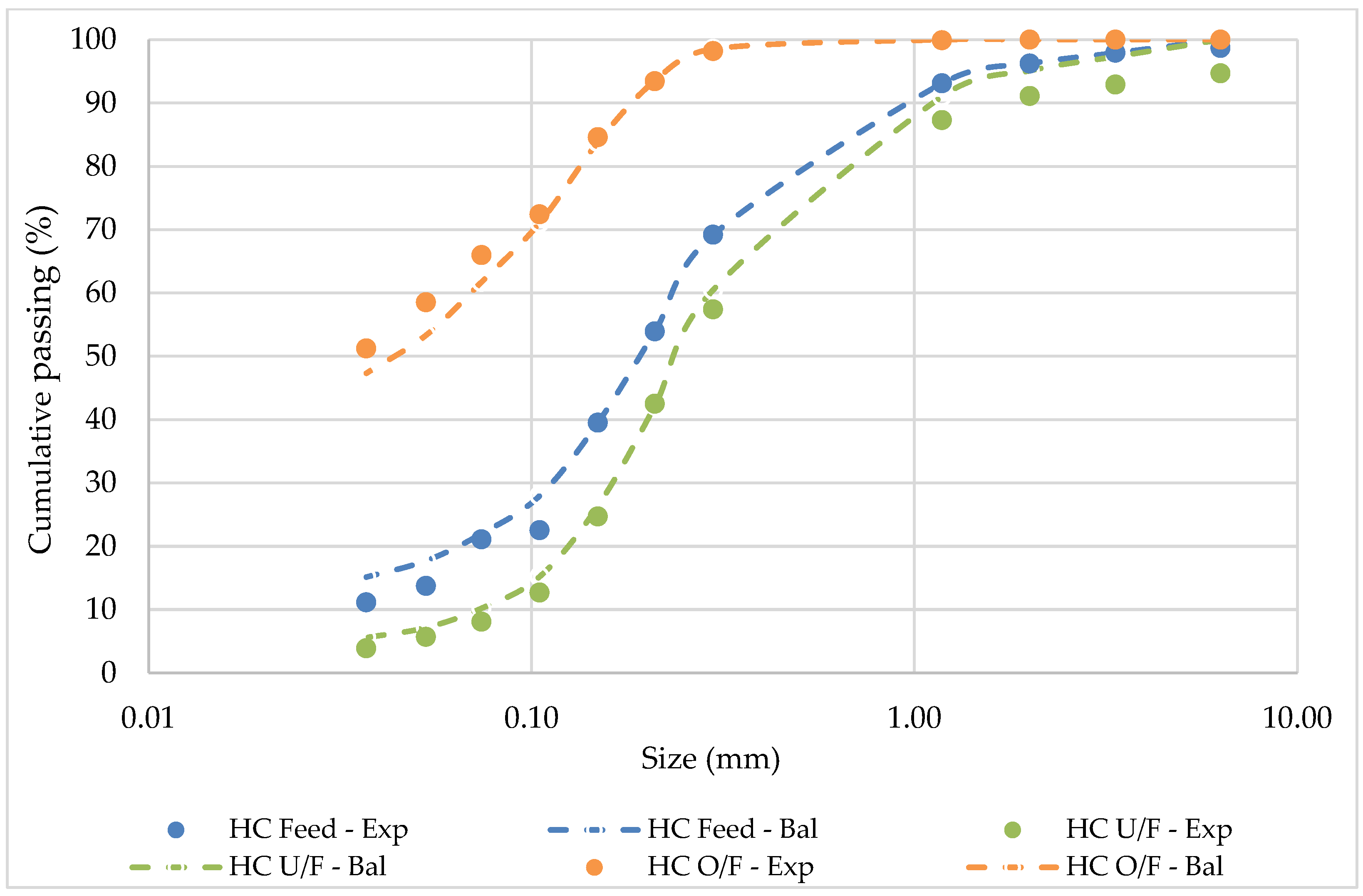
The graph in Figure 5 shows the experimental and mass-balanced size distributions for each stream associated with the HFS+HC configuration.

The graph in Figure 5 indicates five experimental/balanced size distributions. In this case, the HC overflow and HFS feed are the same stream. Except for the HC feed stream, all other streams showed good agreement between their experimental and balanced size distributions. However, the HFS undersize, at 0.150 mm, experimental datum showed a relatively high discrepancy, together with the HC underflow at 2.0 mm. Figure 5 shows a coarser balanced size distribution for the HFS feed in the 0.210 mm to 0.037 mm range compared to the corresponding experimental data. Conversely, the HC feed’s balanced distribution is significantly finer than its respective experimental data for particles finer than 0.210 mm. One plausible reason for such a trend is the difficulty of sampling the HC feed stream in industrial installations.

Table 3. Parameters of partition curves, HFS+HC configuration—Campaign 1.

Size Separation Device	α	d50c (mm)	Water Split to Coarse Product (%)
HFS+HC	3.81	0.140	18.5
HC separated from HFS+HC	1.27	0.217	9.0
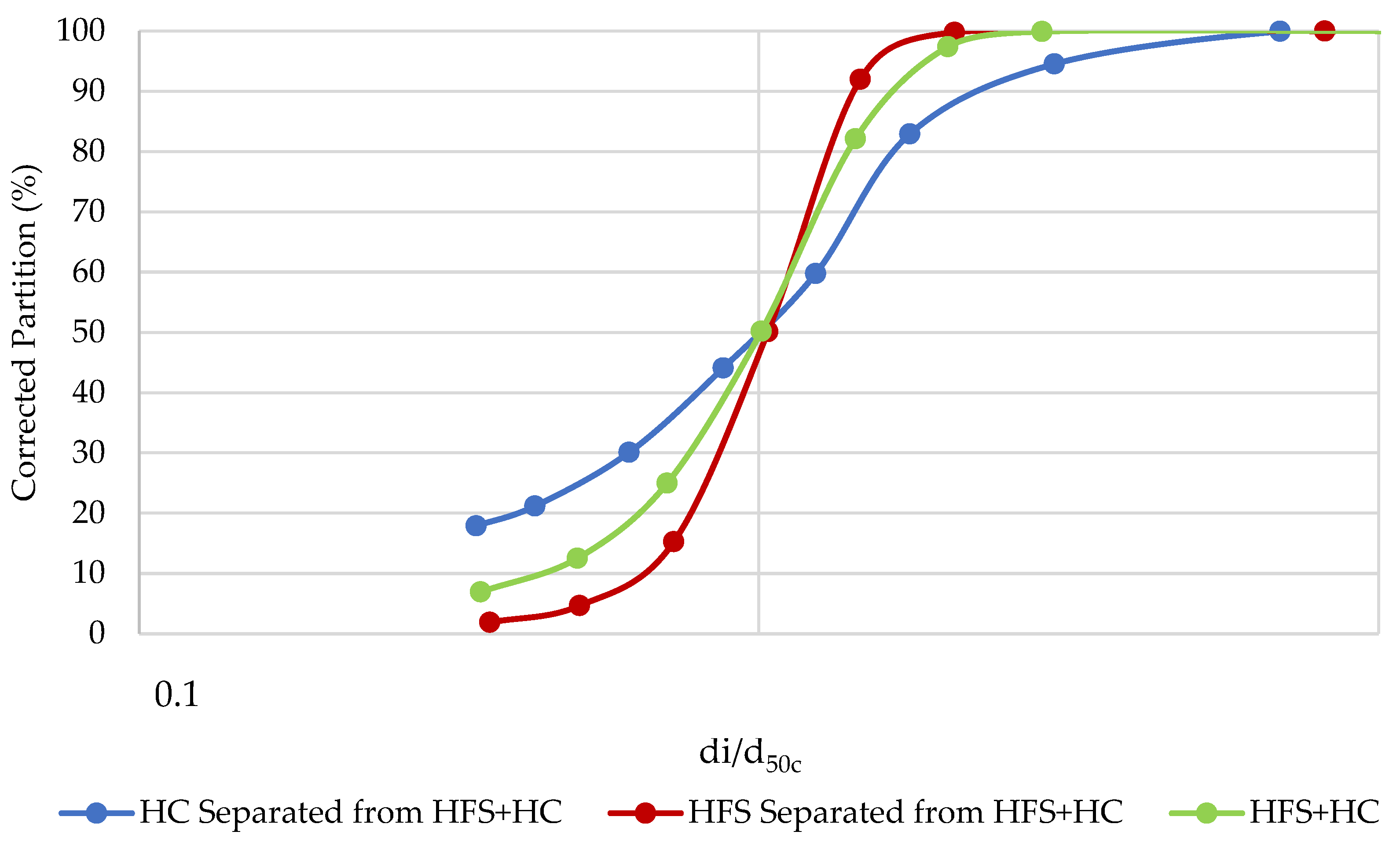
HFS separated from HFS+HC	5.91	0.180	5.6

includes selected parameters derived from both experimental, corrected, and reduced partition curves for the combined operation of HFS+HC and for the decoupled HCs and HFSs within the same operation.

Table 3 shows that the parameter α indicates a sharply reduced partition curve for the combined operation of HFS+HC, representing a high-performance size separation, or an excellent one, as per Table 1. However, individual assessments of the HFSs and HCs in the same circuit configuration resulted in totally different performances, i.e., the HC was considered just reasonable (α = 1.17), while the HFS showed exceptional performance (α = 5.91). Therefore, comparing the separated HFS with the combined HFS+HC configuration clearly shows that the HC operation worsened the size separation performance.

Table 3 also reveals a relatively coarse d_50c for the HC and a fine d_50c for the HFS, resulting in an even finer overall d_50c (0.140 mm). The latter value is very close to the HFS nominal aperture (0.150 mm). A similar pattern is observed for the water split from the coarse product, where exceptionally high performances were achieved for both the HFS and HC, and excellent for the HFS+HC combination, as per the Table 2 criteria.

The graph in Figure 6 shows the calculated reduced partition curves for the same three conditions. The fact that corrected partitions still showed positive values for the corresponding finest particle size in any of the three curves in Figure 6 is attributed to the Kelsall [13] method for bypass calculation, which states that short-circuiting is in direct proportion to the fraction of feed water reporting to the underflow. Using finer screening to assess particle size distributions contributes to mitigating such an aspect, as observed from Figures 9 and 11 onwards.

The HC curve in Figure 6 is significantly dispersed from the vertical line, whose abscissa is 1.0 compared to the HFS+HC and HFS-separated operation curves. In this case, the high dispersion indicates a significant accumulation of coarse particles in the HC fine product (overflow) and a significant accumulation of fine particles in the HC coarse product (underflow).

3.1.2. HC-Only Configuration

The graph in Figure 9 shows the experimental and mass-balanced size distributions for each stream in the HC-Only configuration.

The graph in Figure 7 shows a coarser balanced size distribution compared to the experimental data on the HC overflow in the 0.105 mm to 0.037 mm range. The HC underflow resulted in a finer mass-balanced distribution across the entire size distribution, except the 0.149 mm to 0.210 mm range. Conversely, the HC feed’s balanced size distribution adheres well to its respective experimental data, apart from the 0.149 mm to 0.037 mm range, while the 0.074 mm datum drives the balancing exercise.

Table 4. Parameters of partition curves, HC-Only configuration—Campaign 1.

Size Separation Device	α	d50c (mm)	Water Split to Coarse Product (%)
HC	0.79	0.080	22.3

includes selected parameters derived from the experimental, corrected, and reduced partition curves for the HC-Only configuration.

The α parameter in Table 4 indicates a reduced partition curve with significant dispersion for the HC-Only configuration (α = 0.79), representing a low-performance size separation, or a poor performance, as per Table 1. The d_50c parameter is much finer (d_50c = 0.080 mm) than the equivalent figure obtained for the HC+HFS combined operation, as shown in Table 3 (d_50c = 0.140 mm). The calculated 22.3% water split to coarse product is considered typical of a good separation performance, as per Table 2.

3.2. Second Campaign—May 2023

3.2.1. HFS+HC Configuration

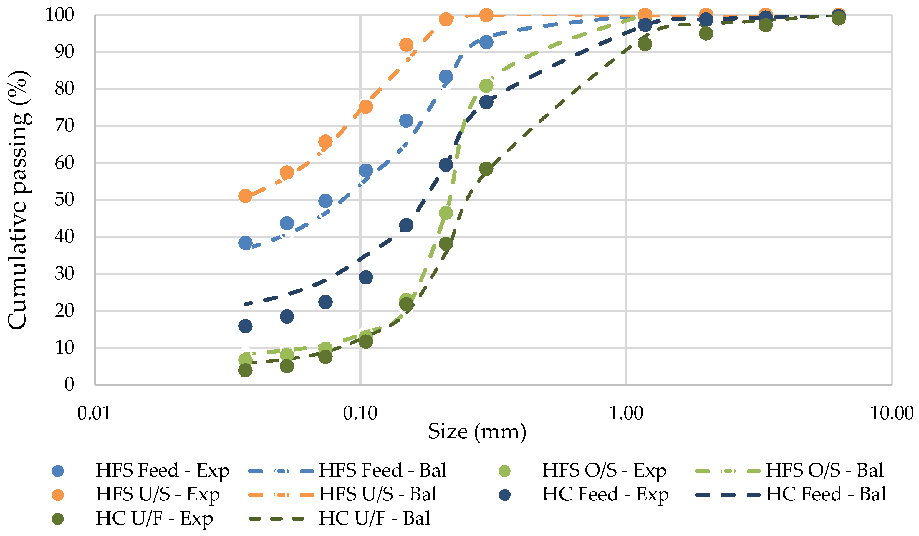
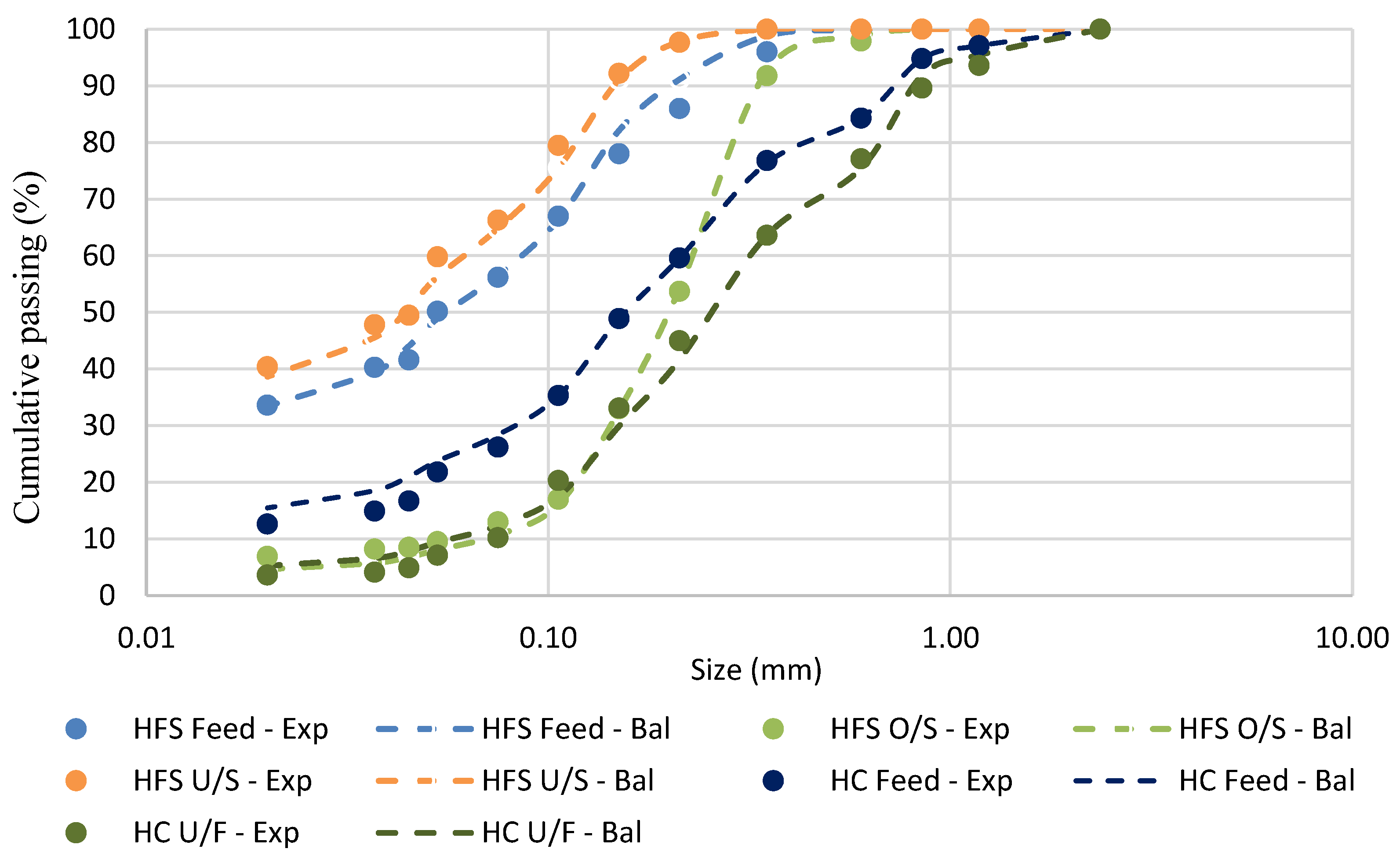
The graph in Figure 8 shows both the experimental and mass-balanced size distributions for each stream associated with the HFS+HC configuration.

The graph in Figure 8 indicates five experimental/balanced size distributions. In this case, the hydrocyclones’ overflow and high-frequency screens’ feed are the same streams. The HFS undersize and the feed streams’ balanced data resulted in a smoother distribution than their corresponding experimental data. In contrast, the HFS oversize indicated a coarser balanced size distribution than the experimental data for sizes finer than 0.075 mm. As observed in Campaign 1, the difficulties associated with sampling the HC feed persisted in Campaign 2.

Table 5. Parameters of partition curves, HFS+HC configuration—Campaign 2.

Scheme 50	α	d50c (mm)	Water Split to Coarse Product (%)
HFS+HC	3.41	0.122	23.8
HC separated from HFS+HC	1.01	0.134	19.2
HFS separated from HFS+HC	4.41	0.209	1.9

includes selected parameters derived from experimental, corrected, and reduced partition curves for the combined operation of HFS+HC and for HC and HFS separately within the same operation.

The α parameter in Table 5 indicates a sharply reduced partition curve for the combined operation of HFS+HC, representing a high-performance, or excellent, size separation, as per Table 1. However, individual assessments of the HFSs and HCs in the same circuit configuration resulted in totally different performances, i.e., the HC was regarded as just reasonable (α = 1.01), while the HFS showed an exceptional performance (α = 4.41). As observed in the Campaign 1 analysis, comparing the separated HFS and the combined HFS+HC configuration clearly shows that the HC operation deteriorated the size separation performance.

Table 5 shows a relatively coarse d_50c for the HFS and a fine d_50c for the HC, resulting in an even finer overall d_50c (0.122 mm). This value is finer than the HFS nominal aperture (0.150 mm). In terms of water split to coarse product, an exceptionally high performance was achieved for the HFS, an excellent performance for the HC, and a good performance for the HFS+HC combination, as per the Table 2 criteria. The graph in Figure 9 shows the calculated reduced partition curves of the three conditions.

Figure 9. Reduced partition curves for HFS+HC and separate HFS and HC conditions—Campaign 2.

Figure 9. Reduced partition curves for HFS+HC and separate HFS and HC conditions—Campaign 2.

As in Campaign 1, the HC curve in Figure 9 is significantly dispersed from the vertical line, whose abscissa is 1.0, compared to the HFS+HC and HFS-separated operation curves, showing, again, that a high dispersion indicates a significant accumulation of coarse particles in the HC fine product (overflow) and a significant accumulation of fine particles in the HC coarse product (underflow).

Analyzing the corrected partition curve, it is possible to notice that, even with the finest sieve (0.020 mm), the bypass continues to exist. This phenomenon can be observed in the corrected partition curves of all samplings carried out in this work, indicating that the Kelsall [13] method has limitations. Therefore, other methods for defining bypass should be investigated.

3.2.2. HC-Only Configuration

The graph in Figure 10 shows the experimental and mass-balanced size distributions for each stream in the HC-Only configuration.

The graph in Figure 10 shows the overall reasonable adherence of the balanced size distribution to the respective experimental data.

Table 6. Parameters of partition curves, HC-Only configuration—Campaign 2.

Size Separation Device	α	d50c (mm)	Water Split to Coarse Product (%)
HC	0.71	0.131	23.5

includes selected parameters derived from experimental, corrected, and reduced partition curves of the HC-Only configuration.

The α parameter in Table 6 indicates a reduced partition curve with a significant dispersion for the HC-Only configuration (α = 0.71), representing a low-performance, or poor, size separation, as per Table 1. The d_50c parameter is coarser than the equivalent figure obtained for the HC+HFS combined operation, as shown in Table 5 (d_50c = 0.122 mm). The calculated 23.5% water split to coarse product is typical of a good separation performance, as per Table 2.

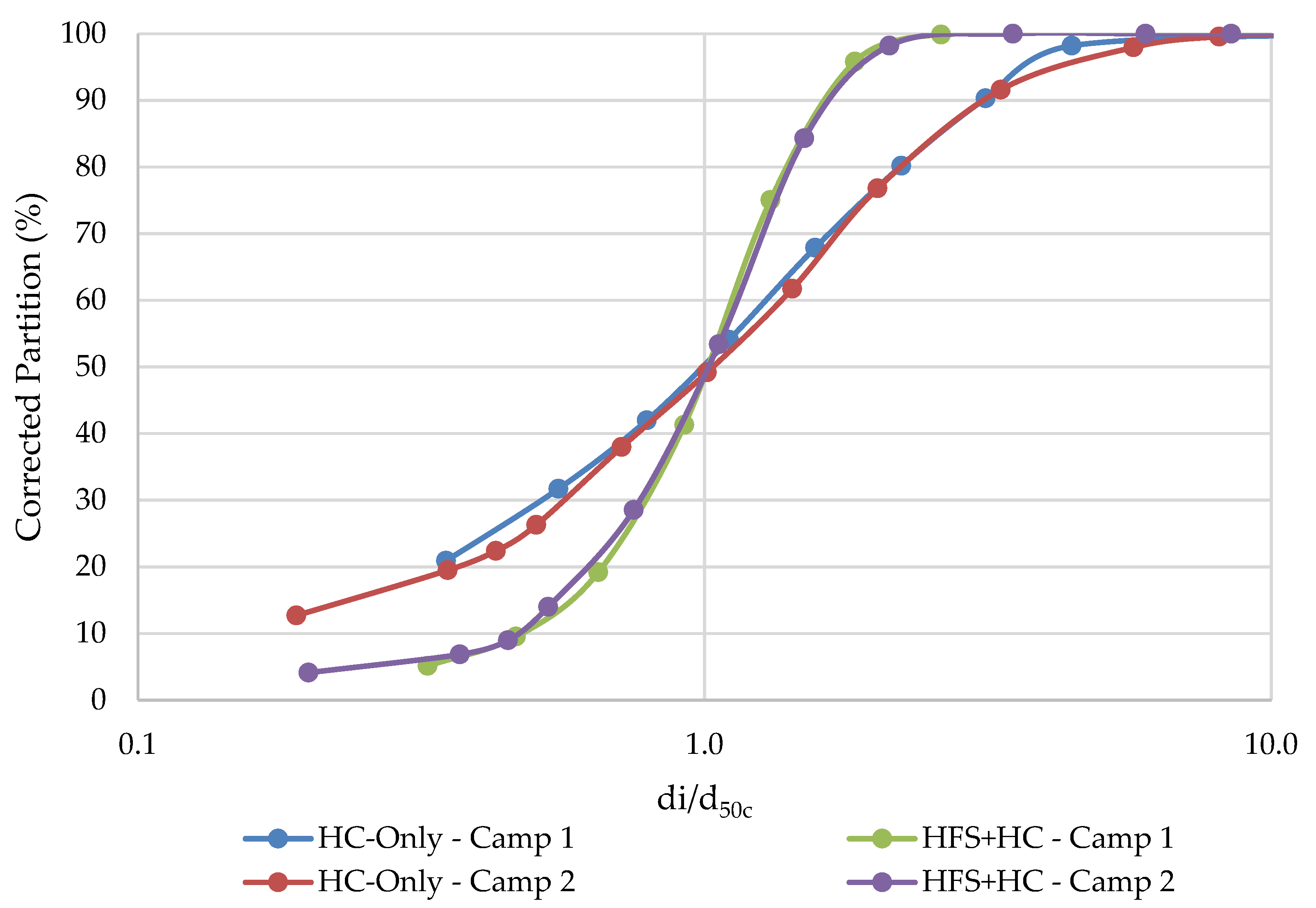
3.3. Comparisons between Campaigns 1 and 2

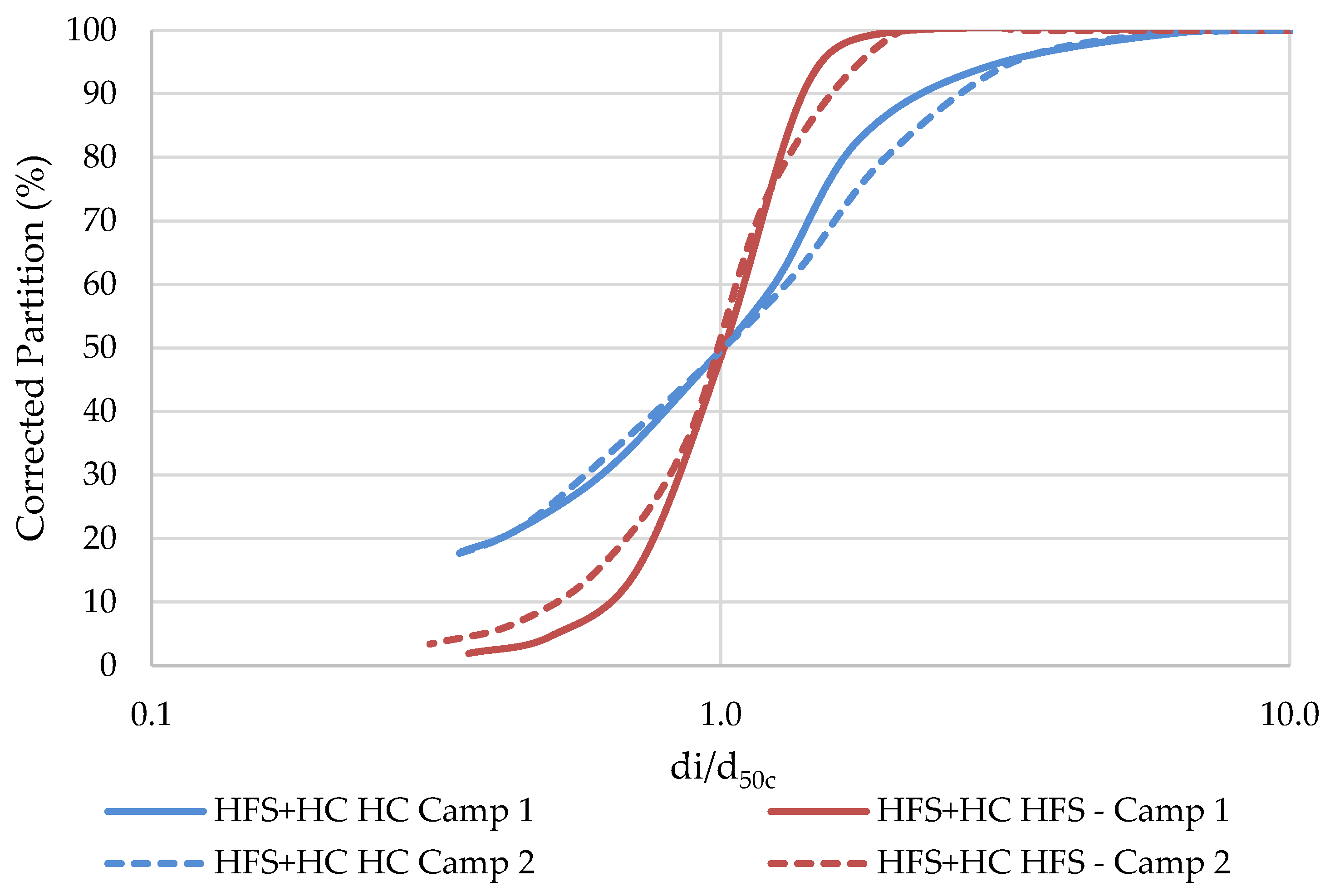
The graph in Figure 11 shows the reduced partition curves obtained for the HFS+HC and HC-Only configurations in Campaign 1 and Campaign 2. Detailed corrected partition data are shown in Table A6 and Table A7 of Appendix C.

Figure 11 illustrates that the HFS+HC configuration resulted in very close reduced partition curves for both campaigns. Similarly, only relatively small differences were observed between the two reduced curves for the HC-Only configuration. The close results obtained from the two campaigns indicate consistent performances.

Figure 11. Reduced partition curves for the HFS+HC and HC-Only configurations—Campaigns 1 and 2.

Figure 11. Reduced partition curves for the HFS+HC and HC-Only configurations—Campaigns 1 and 2.

The comparison between the two configurations indicates that the HC-Only curves are significantly more dispersed from the vertical line, whose abscissa is 1.0, than the HFS+HC curves. This high dispersion in the HC-Only configuration indicates a significant accumulation of coarse particles in the HC fine product (overflow) and a significant accumulation of fine particles in the HC coarse product (underflow).

For further comparisons,

Table 7. Parameters of partition curves of HC+HFS and HC-Only configurations—Campaigns 1 and 2.

Size Separation Device	Campaign	α	d50c (mm)	Water Split to Coarse Product (%)
HFS+HC	1	3.81	0.140	18.5
	2	3.41	0.122	23.8
HC-Only	1	0.79	0.080	22.3
	2	0.71	0.131	23.5

shows the selected parameters calculated from the experimental, corrected, and reduced partition curves of the two configurations in each of the two campaigns.

The similarities between the α parameter in each configuration underpin the close curve shapes observed in Figure 11. The d_50c parameters obtained from the corrected partition curves are relatively close in the HFS+HC configuration, yet notably different for the HC-Only configuration. The latter arises from inconsistent operation and/or the inherent difficulties associated with HC control. Table 7 shows close water split figures for both configurations, with a slightly better performance in the HFS+HC configuration of Campaign 1.

An analogous type of analysis was conducted separately with the HFS+HC configuration. Figure 12 shows the separated reduced partition curves of the HC and HFS, obtained from the HFS+HC configuration for both Campaign 1 and Campaign 2. Detailed corrected partition data can be found in Table A2 and Table A3 of Appendix B. Selected parameters calculated from the experimental, corrected, and reduced partition curves of the two configurations in each campaign are listed in

Table 8. Parameters of partition curves of HC+HFS configurations—Campaigns 1 and 2.

Size Separation Device	Campaign	α	d50c (mm)	Water Split to Coarse Product (%)
HFS+HC - HFS separated	1	5.91	0.180	5.6
	2	4.41	0.209	1.9
HFS+HC - HC separated	1	1.01	0.134	19.2
	2	0.71	0.131	23.5

.

Here, the similar results obtained from the two campaigns also indicate consistent performances. In this case, the α parameters are relatively small for the separated HC, while the same parameter is much greater for the separated HFS, as shown in Table 8. The curve shapes in Figure 12 reinforce these figures.

The d_50c parameter is consistently greater for the separated HFS than the separated HC, while no significant differences were observed in the paired figures. Interestingly, the water split is consistently very low for the separated HFS, while it is good/excellent in both cases of the separated HC. It is emphasized here that the higher the water split into coarse products, the greater the amount of fines in the same stream.

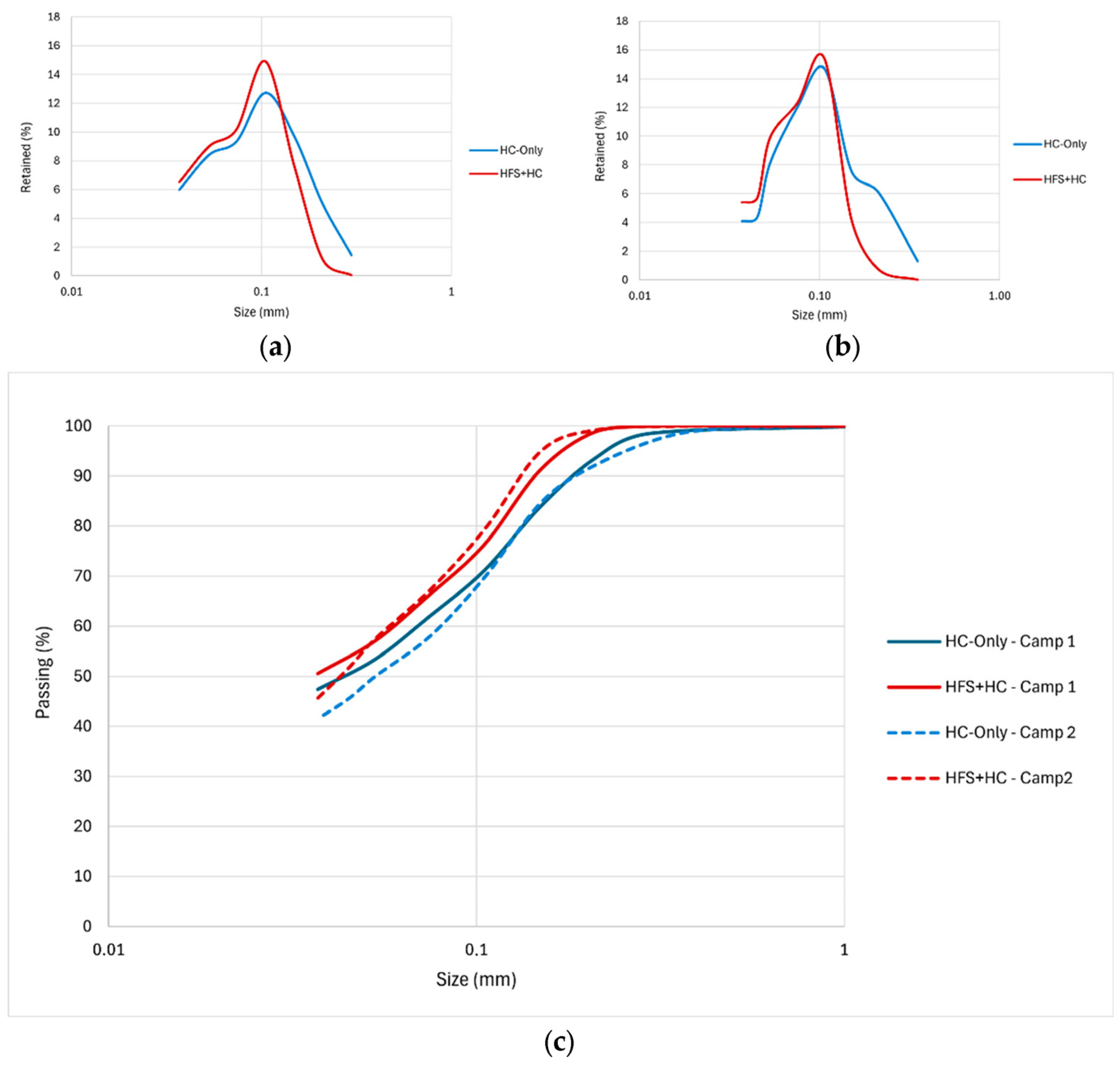
An additional comparison was conducted for the size distributions associated with the circuit configuration. Figure 13 shows the mass-balanced percent retained curves (Figure 13a,b) obtained from both campaigns for the HFS+HC and HC configurations, together with their cumulative percent passing curves (Figure 13c).

Table A8. Size distributions of the grinding circuit product.

Campaign 1			Campaign 2
Size	Retained (%)		Size	Retained (%)
(mm)	HC-Only	HFS+HC	(mm)	HC-Only	HFS+HC
0.298	1.5	0	0.35	1.3	0
0.21	5	1.1	0.212	6.1	0.7
0.149	9.7	7.6	0.15	7.6	4.2
0.105	12.7	14.9	0.106	14.7	15.4
0.074	9.4	10.2	0.075	12	12.3
0.053	8.4	9	0.053	8.1	9.9
0.037	6	6.5	0.045	4.4	5.7
-	-	-	0.037	4.1	5.4

in Appendix D shows detailed data of the two plotted size distributions in Figure 13.

Both the Figure 13a and 13b curves peak at 0.10 mm, apart from other inflection points. Even though more emphasis is placed on Campaign 1 than Campaign 2, the HFS+HC configuration shows a greater mass accumulation than the HC-Only configuration for the same particle size.

A more important aspect of both graphs is the significantly higher mass amounts in the HC-Only curves’ coarser ends. This indicates higher contents of coarse particles in the HC-Only configuration grinding circuit product than in the HFS+HC configuration, with the former thus showing a higher potential for unliberated particles in the grinding circuit product. The same graphs (a) and (b) in Figure 13 also show greater amounts of particles in size fractions finer than 0.10 mm.

4. Conclusions and Recommendations

The two comprehensive survey campaigns of Nexa’s Vazante C grinding circuit resulted in consistent performances associated with the HC-Only and the HFS+HC hybrid configurations. The HC-Only configuration showed a significantly deteriorated performance, with higher contents of finer particles in the coarse product and higher contents of coarser particles in the fine product compared to the HFS+HC configuration. This conclusion was based on comparisons of the calculated dispersion parameter from the Whiten equation used to parameterize the respective reduced partition curves, along with the water split to the coarse product. While the former was significantly higher for the HFS+HC configuration, indicating a smaller dispersion, the latter was higher for the HC-Only configuration, which clearly indicates higher fines in the coarse product.

Further assessments of the decoupled HCs and HFSs in the HFS+HC configuration showed the same pattern: a substantially poor performance of the HCs compared to the excellent performance of the HFSs, as indicated by the partition curve dispersion parameter and water split to coarse product. In both campaigns, comparing the separated HFS and the combined HFS+HC configuration clearly demonstrated that the HCs’ operation was detrimental to the circuit’s size separation performance. A greater separation efficiency allows for an increase in the mass processed in the grinding circuit and, consequently, a reduction in the energy spent per ton treated.

The grinding circuit product associated with each configuration was also compared. The HFS+HC configuration resulted in a higher concentration of particles in the targeted 0.10 mm particle size range. In contrast, the HC-Only configuration had relatively greater amounts of particles in size fractions coarser than 0.10 mm and a smaller mass in size fractions finer than 0.10 mm. The former indicates a potential source of unliberated particles, while the latter indicates overgrinding, which is detrimental to the downstream concentration stages.

The results showed that the combined use of sieves and cyclones increases the generation of 0.037 mm particles in the product by around 2% to 3%, which could worsen flotation performance and increase reagent consumption, given that the metallurgical recovery for this fraction is 83.5%. However, the reduction in the coarse fraction (0.212, 0.150, and 0.106 mm) reaches up to 8%. Since the recovery of these fractions is extremely low (27.7%, 48.9%, and 81.5%, respectively), the gain from using a combined sieve and cyclone compensates for the generation of fines in this configuration. A second article will assess the metallurgical performance of the two different product size distributions in detail.