Article

Leveraging Domain Expertise in Machine Learning for Critical Metal Prospecting in the Oslo Rift: A Case Study for Fe-Ti-P-Rare Earth Element Mineralization

by
Ying Wang
*,
Nolwenn Coint
,
Eduardo Teixeira Mansur
,
Pedro Acosta-Gongora
,
Ana Carolina Rodrigues Miranda
,
Aziz Nasuti
and
Vikas Chand Baranwal
Geological Survey of Norway (NGU), Leiv Eirikssons vei 39, 7040 Trondheim, Norway
*
Author to whom correspondence should be addressed.
Minerals 2024, 14(4), 377; https://doi.org/10.3390/min14040377
Submission received: 4 March 2024 / Revised: 31 March 2024 / Accepted: 31 March 2024 / Published: 3 April 2024

Abstract

:
Global demand for critical raw materials, including phosphorus (P) and rare earth elements (REEs), is on the rise. The south part of Norway, with a particular focus on the Southern Oslo Rift region, is a promising reservoir of Fe-Ti-P-REE resources associated with magmatic systems. Confronting challenges in mineral exploration within these systems, notably the absence of alteration haloes and distal footprints, we have explored alternative methodologies. In this study, we combine machine learning with geological expertise, aiming to identify prospective areas for critical metal prospecting. Our workflow involves processing over 400 rock samples to create training datasets for mineralization and non-mineralization, employing an intuitive sampling strategy to overcome an imbalanced sample ratio. Additionally, we convert airborne magnetic, radiometric, and topographic maps into machine learning-friendly features, with a keen focus on incorporating domain knowledge into these data preparations. Within a binary classification framework, we evaluate two commonly used classifiers: a random forest (RF) and support vector machine (SVM). Our analysis shows that the RF model outperforms the SVM model. The RF model generates a predictive map, identifying approximately 0.3% of the study area as promising for mineralization. These findings align with legacy data and field visits, supporting the map’s potential to guide future surveys.

1. Introduction

The global demand for critical raw materials has been steadily increasing due to their essential role in high-tech industries [1,2]. Among these materials, rare earth elements (REEs) and phosphorus (P) are listed as critical raw materials by the European Union [3], underscoring their significance as strategic resources for the future. The REEs stand towards the top of the priority list due to their use in various green-energy technologies, whereas P plays a critical role in the fertilizing industry.
In this context, the geological setting of Norway displays great potential for the discovery and subsequent exploitation of critical raw materials, especially P-REE resources [4]. Notably, significant Fe-Ti-P-REE resources have been identified in Norway that are related to layered intrusions and alkaline intrusive complexes [5,6], emphasizing the potential for discoveries in diverse settings. The Southern Oslo Rift region is renowned for hosting multiple magmatic occurrences that are rich in Fe-Ti-P-REE, with the Kodal deposit being the largest and most well-known to date [7]. However, as most of these resources are formed as part of magmatic systems, targeting new discoveries is often hampered by the absence of extensive alteration haloes or distal footprints, as for example observed in hydrothermal systems. Therefore, developing alternative exploration tools is critical for supporting new future discoveries.
Machine learning has emerged as a powerful tool in the field of mineral potential mapping, and its successful applications have been reported across the world [8,9,10,11,12,13]. One of its primary strengths in this context lies in its capacity to efficiently handle extensive and intricate multivariate datasets, a substantial improvement over traditional methods. Furthermore, machine learning allows for objective data integration, reducing the potential biases that can arise from human expertise. However, there are also potential limitations associated with this data-driven approach [14,15]. In mineral exploration, it can be challenging to train models effectively due to limited and biased data. Typically, there are more negative cases (non-mineralized) than positive cases (mineralized), simply due to the rarity of mineral resources, and the available data may be incomplete. For instance, only confirmed positive samples (known mineralization) may be available, and negative samples (rocks devoid of mineralization) must be randomly selected and/or conform to specific empirical guidelines from the area of interest. These factors can impact the accuracy and reliability of the models used in mineral exploration [16,17,18]. Machine learning models are often considered as ‘black boxes’, meaning it can be difficult to understand how the algorithms arrive at their predictions from the multi-variate features or how these features are associated with the underlying geological processes that control the mineralization. In this contribution, we address these limitations and combine data science with geological domain expertise in developing our predictive model.
This study is dedicated to employing a machine learning approach to identify potential areas for early-stage exploration of Fe-Ti-P-REE resources within the Southern Oslo Rift region. Existing high-resolution spatial datasets, including airborne magnetic, radiometric, and topographic maps, were used to generate predictive features, and rock samples with geochemical analyses were processed into training samples. For the generation of the predictive model, two widely used classifiers were evaluated: a random forest (RF) [19], which is splitting-based, and a support vector machine (SVM) [20], which is continuity-based. Both classifiers were implemented with modifications to handle imbalanced datasets (i.e., there are significantly more negative samples than positive ones) by adjusting the class weights based on the class frequencies and adjusting the cost matrix to penalize assigning samples to the overrepresented class (negative, non-mineralized) more heavily. The RF classification model was selected due to its superior performance, and the generated predictive map was compared to the legacy data and verified in the field. This was proven to be valuable in terms of narrowing down areas that require further investigation for mineral exploration.

2. Geological Background of the Study Area

The study area is located at the Oslo Rift in the southeastern part of Norway, in the vicinity of the cities of Skien, Sandefjord, and Larvik, covering about 2000 km2 (Figure 1).
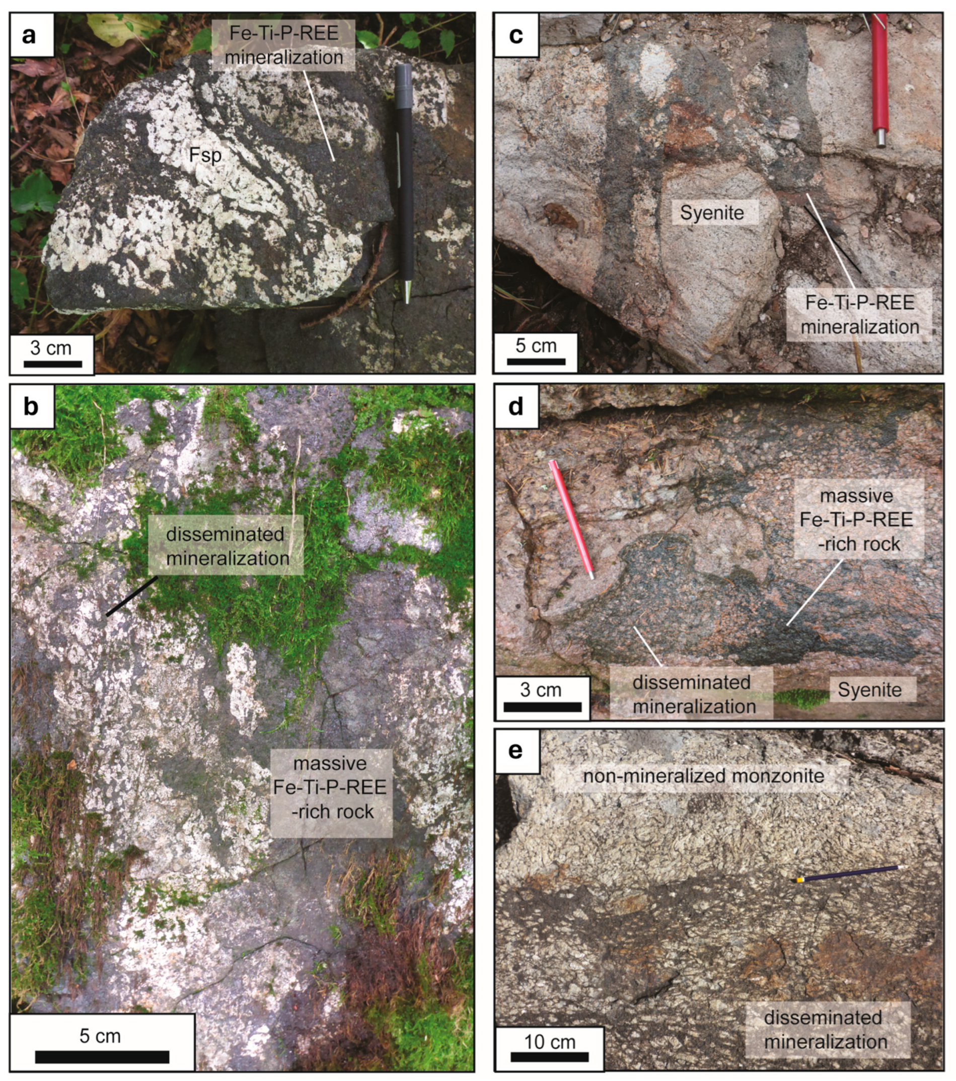
The Oslo Rift hosts some of the youngest magmatic rocks of the Fennoscandian Shield, formed between 302–256 Ma [21,22,23,24]. The magmatic activity in the rift began with the emplacement of the B1 basalts [25], some of which crop out in the study area, close to Skien. This was followed by the emplacement of voluminous trachytic and trachyandesitic lava flows characterized by their rhomb-shaped alkali feldspar phenocrysts (rhomb porphyry lava), thereafter intruded by the Larvik Plutonic Complex (LPC) between 296 and 289 Ma [24] and younger monzonitic to quartz-bearing syenitic intrusions (Siljan-Hvarnes intrusion-SHI, 277–281 Ma) [26]. Several occurrences of Fe-Ti-P-REE-rich rocks (examples in Figure 2) have been described to be associated with the intermediate to felsic magmatism [5,27], including the Kodal Fe-Ti-P-REE ore deposit (Figure 1c).
The Kodal deposit represents the largest known occurrence of Fe-Ti-P-REE mineralization in the LPC, with total indicated resources of 14.6 Mt at 5.18% P2O5 and 24.12% Fe [7]. Moreover, apatite from the deposit hosts between 0.92 to 1.29 wt.% total rare earth oxide potential by-products [4]. The western part of the deposit is exposed, where massive titanomagnetite–apatite–ilmenite-rich rocks (main mineralization) can be observed. The ore varies from a few centimeter intervals that occur as pockets within the monzonite, displaying sharp contacts, to zones with approximately 2 m of thickness, normally surrounded by disseminated intervals (Figure 2a,b). Around 40 cores were drilled in the Kodal deposit in the early 1980s, providing valuable insights into the geometry of the mineralization. Whole-rock geochemical analyses for the cores yield on average 1.33 wt.% P2O5, 12.3 wt.% Fe2O3, and 2.4 wt.% TiO2 for the host monzonite, 2.7 wt.% P2O5, 19.1 wt.% Fe2O3, and 4.18 wt.% TiO2 for the disseminated ore, and 7.3 wt.% P2O5, 44.7 wt.% Fe2O3, and 8.63 wt.% TiO2 for the massive ore. Thus, the limit between the host rock and the ore is mostly based on Fe2O3, TiO2, and P2O5 concentrations.
Other Fe-Ti-P-REE mineralization with similar characteristics to the Kodal deposit have been described in the Oslo Rift region. These include in the Siljan intrusion [28] (Figure 1 and Figure 2c,d), where the P content reaches up to 5 wt.%, and a locality along the shore of Lake Farris in Kjose (Figure 2e). The extent of the mineralization in these occurrences, however, is poorly constrained. Nonetheless, their presence underscores the possibility of mineralization in intrusions beyond the LPC.
Based on the results from previous regional studies [5,27] and especially known mineralization sites such as Kodal [29,30], it is possible to identify the critical parameters that characterize the Fe-Ti-P-REE mineralization in the area. For instance, due to abundant magnetite, the mineralization is characterized by positive magnetic anomalies (1000–3000 nT), whereas a low content of potassium (K)-rich minerals yields lower K concentrations (generally below 2%) relative to the host rocks. Moreover, the mineralization seems to be more promptly eroded relative to the host rocks, thus being present in topographic depressions of secondary importance. These contrasting petrophysical properties of the ore compared to the host rock make this type of mineralization prone to be detected using various classical geophysical exploration tools such as radiometric and magnetic surveys.

3. Data

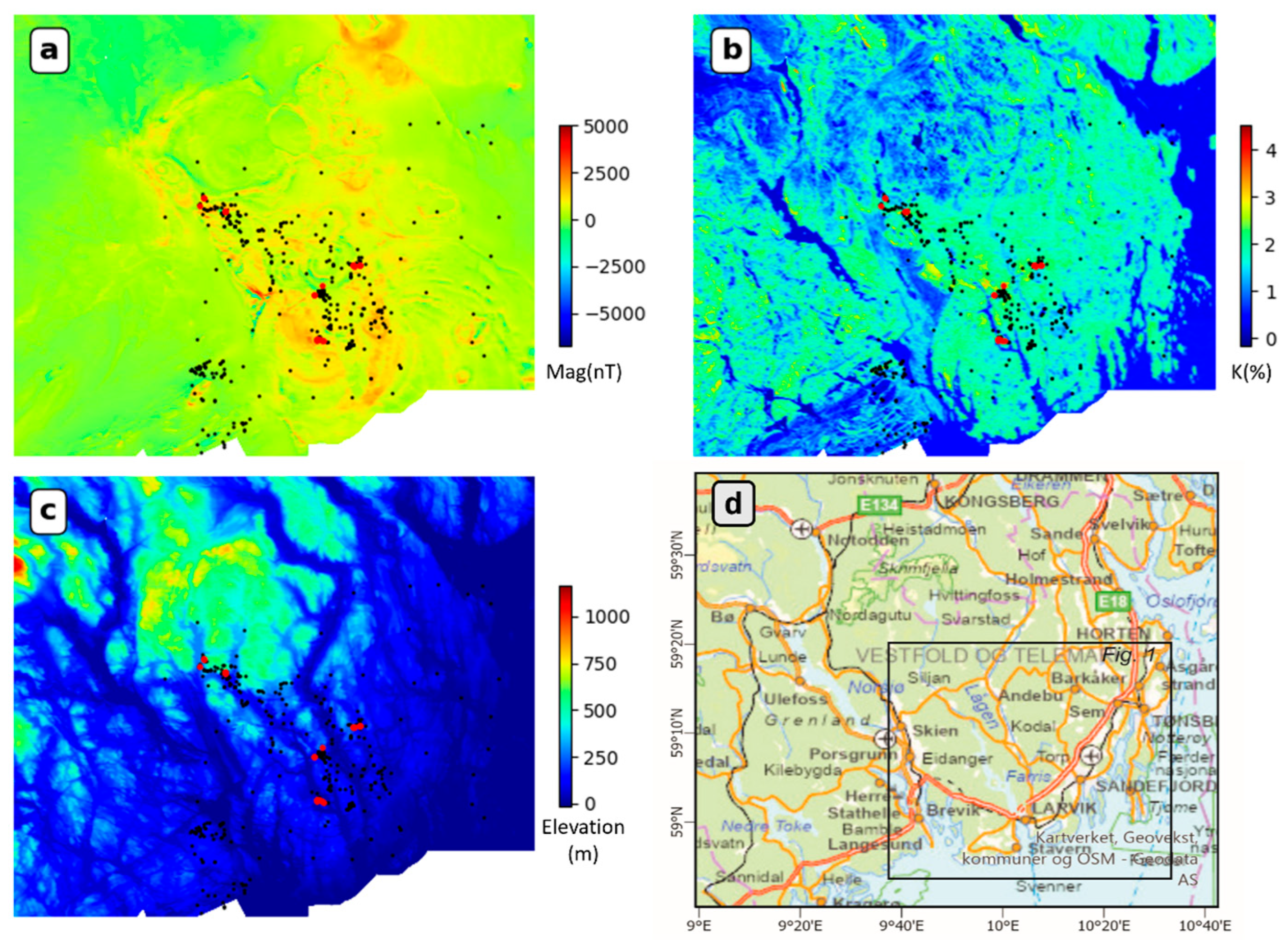
This study utilizes high-resolution geospatial datasets, including airborne geophysics and the digital elevation model (DEM), to create a set of features as the input to our machine learning model. Based on the domain knowledge described in Section 2, these features are likely indicative of the target mineralization, enabling us to build a robust predictive framework for a mineralization prospectivity assessment. To prepare the geospatial datasets and based on data availability, we extended the coverage beyond the study area, as shown in Figure 3d. The magnetic and radiometric airborne geophysical datasets are compiled and stitched from multiple surveys conducted at different times [31]. The compilations are provided by the Geological Survey of Norway (NGU) (https://geo.ngu.no/geoscienceportalopen/Search accessed on 28 January 2023), which have a regular grid sampling resolution of 50 m. The magnetic data display the total magnetic field anomaly (Figure 3a), while the radiometric data indicate the abundance of potassium (K), thorium (Th), and uranium (U) in rocks and soils. An example of processed K data in weight percentage is presented in Figure 3b. For the DEM data used in this study (Figure 3c), we obtained them from the Norwegian Mapping Authority (Kartverket) at a spatial resolution of 50 m (https://hoydedata.no/LaserInnsyn2/ accessed on 25 January 2023). To ensure spatial alignment of the features used in developing the predictive model, all datasets were projected onto a uniform grid with a cell size of 50 m.
To ensure a comprehensive training dataset, geologists were advised to collect and identify both positive and negative samples across different geological units for good spatial coverage. To be more specific, the rock samples used in this study were collected as part of a mineral resource project aimed at understanding the formation and characterizing the Fe-Ti-P-(REE) occurrences within the region. The geologists sampled various lithological units present in the area, including areas of mineralization, with samples predominantly sourced from locations along accessible roadsides. In addition, the samples are denser close to mineralized areas for petrogenetic purposes. Such datasets are typical in geological surveys conducted for regional-scale studies. Geochemical data consisting of ICP-MS (inductively coupled plasma mass spectrometry) analyses from these field samples were used to measure the concentration of elements of interest in the rocks. The methodology for the analyses followed that reported in reference [32]. During the data preparation stage, mineralogists were consulted to separate the samples into positive and negative training datasets using geochemical and mineralogical indicators. Specifically, building upon the analyses of rock compositions in previously examined drilled cores, as discussed in Section 2, and taking into account the significant abundance of apatite in the mineralized samples, we categorized our field samples based on their P2O5 concentrations. Samples with P2O5 contents exceeding 4 wt.% were classified as mineralized, whereas those with P2O5 contents below 4 wt.% were categorized as non-mineralized. These classified samples were used as the ground truth to develop a training dataset for our predictive model. Of the collected samples, 23 were classified as mineralized, whereas 406 were classified as non-mineralized. The distribution of the classified samples is marked in Figure 3a–c on top of the geospatial maps.

4. Methodology and Workflow

4.1. Training Data Sampling Strategy

Figure 3a–c illustrate a noteworthy advantage of our collected samples: their spatial distribution provides extensive coverage and a substantial proportion of confirmed negative samples. This eliminates the need for generating synthetic negative samples using techniques like SMOTE [18] or blind sampling. However, the field samples present a notable imbalance, with a ratio of 23:406 (≈1:18) between the mineralized samples (i.e., positive) and non-mineralized samples (i.e., negative). This imbalance presents a challenge when training a classification model, as the model tends to learn better at predicting the majority class [33,34]. However, for mineral prospectivity mapping, correctly identifying the minority class (i.e., mineralized samples) is of greater importance. To address this issue, we designed a sampling strategy to generate a training dataset that takes into account the imbalanced data.
We started by assigning class labels (mineralized or non-mineralized) to the surrounding grid cells of the field samples from the uniform grid of 50 m resolution mentioned in Section 3. We chose a 50 m spatial range around the non-mineralized field samples to be assigned as the negative training data, whereas we chose a larger spatial range of 100 m for the mineralized field samples to be assigned as the positive samples. An example of this is illustrated in Figure 4, where Figure 4a shows the grid cells within a 50 m distance from the non-mineralized samples in green, and Figure 4b shows the grid cells within a 100 m distance from the mineralized samples in magenta. In cases of overlapping grid cells, the positive samples overrule the negative samples, as shown in Figure 4c.
Our choice of spatial range sizes is rather conservative because it assigns relatively small spatial extents to the samples. This approach aims to exploit the full potential of the high-resolution features to enable a more subtle spatial differentiation between the mineralized and non-mineralized samples. This sampling scheme is also reasonable in the context of mineral exploration because if both mineralized and non-mineralized samples are found close to each other at a given location, the location would still be considered as having the potential of hosting a larger volume of mineralized rocks (i.e., positive prospectivity indication).
The final training dataset has a ratio of 174:997 (≈1:5.7) between the positive (mineralized) and negative (non-mineralized) samples, which is still imbalanced but much improved from the initial ratio.

4.2. Feature Engineering

Feature engineering is a crucial process in machine learning, involving the extraction of relevant features from raw data to improve model performance. In this study, a collaborative effort among geoscientists with expertise in geophysics, geology, and mineralogy was undertaken to identify significant features from the three high-resolution gridded geospatial datasets (shown in Figure 3) that are likely associated with the target mineralization.
For the magnetic data, we applied several filtering techniques to create features that are routinely used by human experts to help facilitate map interpretation [35]. For example, the upward continuation preserves the low-frequency component of the magnetic data and accentuates deeper sources of magnetism; the analytical signal highlights high-frequency signals coming from shallow sources; and various derivative-based filters, such as vertical and tilt derivatives, enhance the edges of the magnetic anomalies. When necessary, histogram equalization or logarithmic transformation was used to adjust the data distribution with the purpose of improving the features’ discriminatory power. The visual effect of this is the enhanced global contrast in an image view. For instance, Figure 3a presents the original magnetic data in a linear color scale, whereas Figure 5a shows the histogram-equalized version, revealing many more details of the original image. In total, we generated five features from the original magnetic map as candidate features to be input into our machine learning models. These features, shown in Figure 5, include: (a) the histogram-equalized magnetic data (mag_ft), (b) the analytical signal with logarithmic transformation (mag_as_ft), (c) the upward continuation at 500 m (mag_uc500), (d) the vertical derivative with histogram equalization (mag_vd_ft), and (e) the tilt derivative (mag_tdr) of the magnetic data.
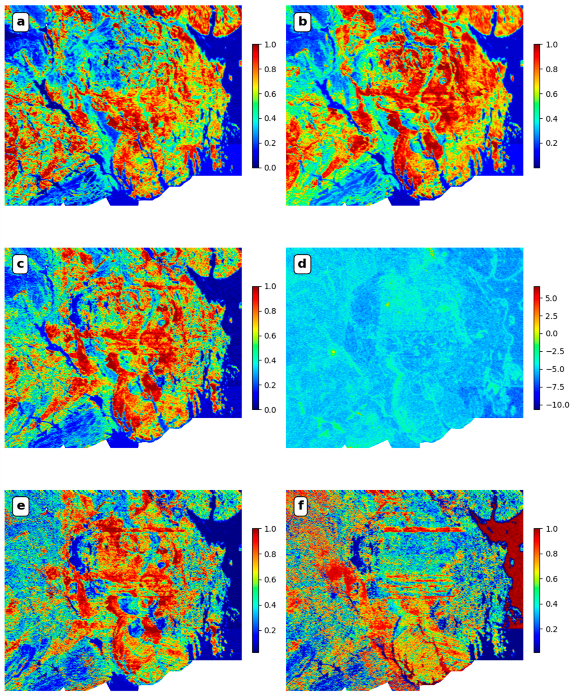
For the radiometric data, the downloaded products represent potassium (K) in weight percentage (%), and uranium (U) and thorium (Th) in their equivalent concentrations of the parent nuclides, referred to as equivalent U (eU in ppm) and equivalent Th (eTh in ppm), respectively, as commonly discussed in the literature [36]. We have assessed the individual radioactive element channels, namely K, eTh, and eU, for their absolute surface concentrations and ratios, i.e., eTh/K, eU/K, and eU/eTh, which indicate their relative concentrations. The ratio operation often amplifies channels with low count rates compared to other channels. As a result, anomalous areas can be highlighted, in contrast to the cases where individual channels are typically correlated in most rock types [37]. Six features were generated from the original radiometric data. The three histogram-equalized individual element channels were K_ft, Th_ft, and U_ft, shown in Figure 6a–c, respectively. The remaining three features were ratios, labelled Th_K_as_ft, U_K_ft, and U_Th_ft, shown in Figure 6d–f, respectively. To generate the Th_K_as_ft feature, we applied a logarithmic transformation to the analytical signal of the ratio eTh/K. The U_K_ft and U_Th_ft features were generated by adding a small constant to the denominator to avoid division by zero and then performing histogram equalization. The decision to use the analytical signal of the ratio of Th/K was influenced by domain experts who found that it better explained the spotted mineralization occurrences than the ratio itself.
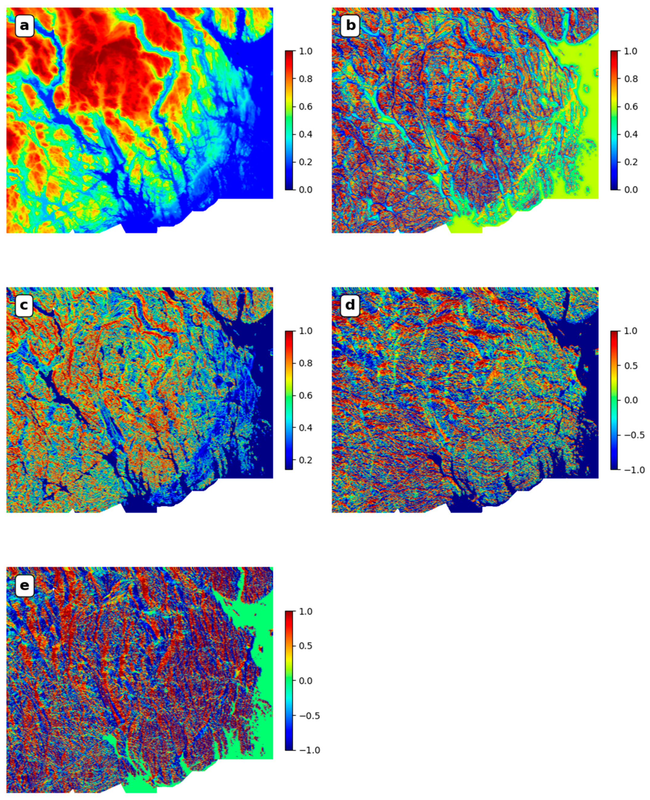
We generated five predictive features from the topographic data. Figure 7a shows the histogram-equalized DEM (Topo_ft), whereas Figure 7b,c display the histogram-equalized vertical derivative (Topo_vd_ft) and slope (Topo_slope_ft) of the DEM data, respectively. The topographic aspect that represents the direction facing the downhill slope was also calculated. However, the aspect values range from 0° and 360° and are circular in nature, meaning that the minimal and maximal aspects of 0° and 360° are essentially the same (due north). To obtain a more interpretable representation of the slope direction in the linear axes, we split the aspect into two features: the sine and cosine components, shown in Figure 7d,e, respectively. The sine component ranges from 1 to −1, representing north-south facing slopes, with 1 indicating due north-facing slopes and −1 indicating due south-facing slopes. The cosine component represents east-west-facing slopes and has the same interpretation.

4.3. Feature Selection

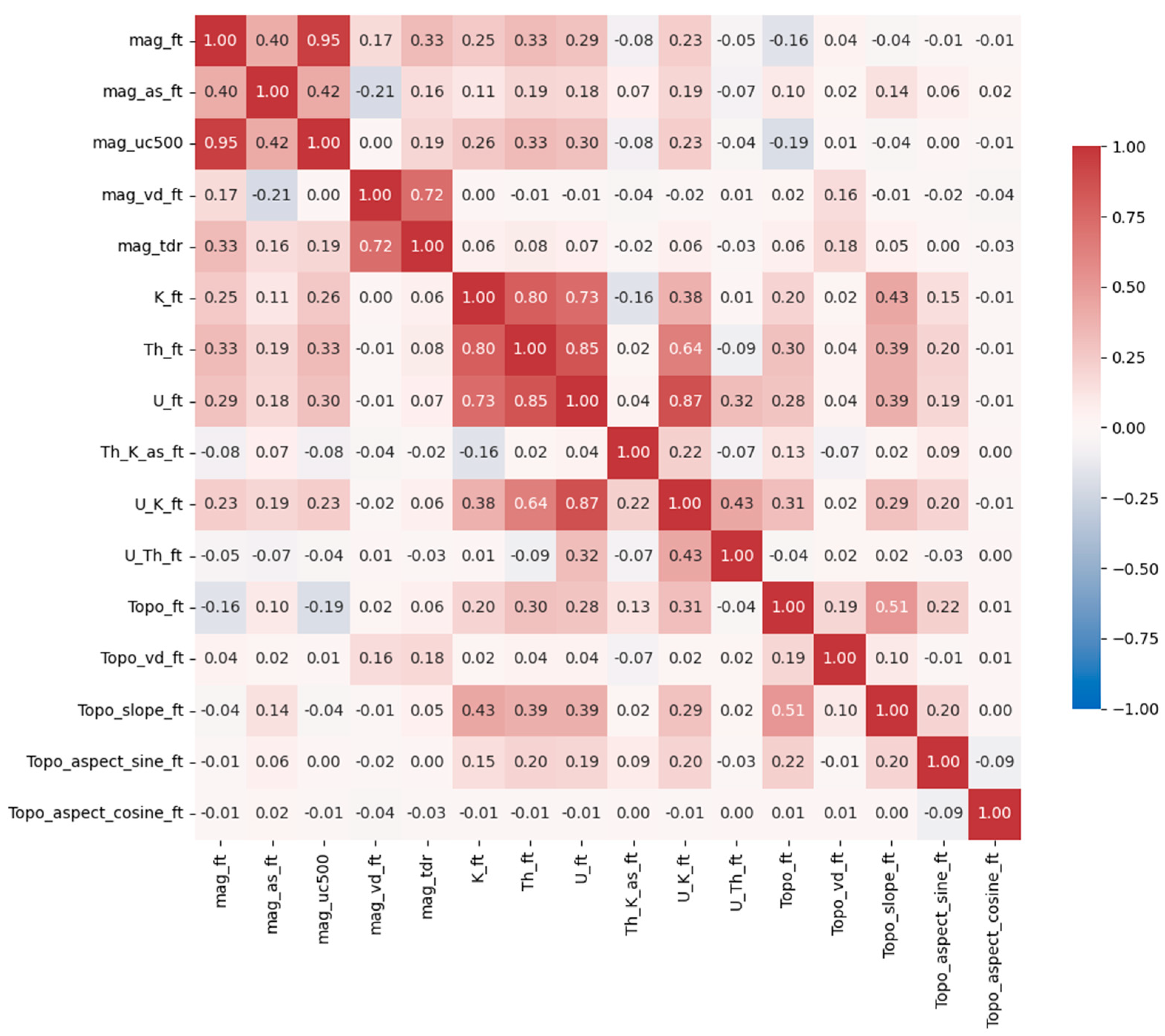
We generated a 2D correlation matrix of all the candidate features (16 in total, described in Section 4.2) using the Pearson’s correlation coefficient, shown in Figure 8. The matrix contains values ranging from −1 (perfect negative correlation) to +1 (perfect positive correlation), with 0 indicating no correlation. To avoid overrepresentation and redundant predictors, we only selected independent and uncorrelated features for building the classification models, with the goal of improving model performance [38]. We set a threshold of 0.7 for the correlation coefficient and discarded four features (mag_ft, mag_tdr, Th_ft, and U_ft) that showed strong correlations with other features, which could be easily identified from the matrix in regions with darker red colors. In summary, the 12 chosen features include 3 magnetic features (mag_as_ft, mag_uc500, and mag_vd_ft), 4 radiometric features (K_ft, Th_K_as_ft, U_K_ft, and U_Th_ft) and 5 topographic features (Topo_ft, Topo_vd_ft, Topo_slope_ft, Topo_aspect_sine_ft, and Topo_aspect_cosine_ft).

4.4. Classification Model

Following the creation of a training dataset consisting of 174 samples labelled as mineralized and 997 samples labelled as non-mineralized, each supported by a 12-dimensional feature vector, a classification model was trained. Twenty percent of the samples (235) were set aside for testing, and the remaining 80% (936) were used for training and validation. Spatial stratified sampling was used to ensure that the samples in close proximity were not split between the training and testing sets. The proportion of mineralized and non-mineralized samples was preserved in both sets using stratified random sampling.
In principle, all well-established classification methods have the potential to accurately solve classification problems, but they differ in their assumptions about the data and modelling hypothesis. For example, decision trees employed in a random forest (RF) split predictive features into discrete, non-overlapping groups, represented by the tree’s leaf nodes, while support vector machine (SVM) uses a hyperplane to separate data into different classes, allowing for flexible modelling of non-linear relationships. Both methods are powerful for modelling complex data, and their respective approaches are equally acceptable for our study. Therefore, we tested both RF and SVM on our classification problem. In practice, we utilized the widely used scikit-learn Python package (version 1.2.2) for the implementation of the RF and SVM algorithms. Both classifiers were implemented with modifications to handle imbalanced datasets by adjusting class weights as inversely proportional to class frequencies and adjusting the cost matrix to penalize assigning samples to the overrepresented class (non-mineralization samples) more heavily.
For both models, we conducted successive training tests by tuning the parameter space over a range of values. For RF, we varied the number of trees and minimum leaf node size, while for SVM, we tested different kernel functions and tuned the regularization parameter. The average accuracy and F1 score were used to evaluate the models under a 5-fold cross-validation scheme. With the optimal model parameter settings, the RF model achieved an average accuracy of 0.949 and an F1 score of 0.815, while the SVM model gave an average accuracy of 0.775 and an F1 score of 0.538. Furthermore, we evaluated the performance of the winning model, the RF model, on unseen data, i.e., the testing set that we set aside, and it achieved an overall accuracy of 0.962. Specifically, we checked the confusion matrix, which gave us a classification accuracy of 0.900 for the positive (mineralized) samples and 0.971 for the negative (non-mineralized) samples. In the Supplementary Material, Figure S1, we also included the receiver operating characteristic (ROC) curve of the RF model to demonstrate its discriminative performance and highlight its ability to distinguish between positive and negative instances in our analysis. This graphical representation serves as an additional visual aid to underscore the effectiveness of the RF model in the context of this study. This result gave us assurance about the RF model’s performance regarding over-fitting and handling of the imbalanced dataset. Therefore, we chose the trained RF model to predict the mineral potential of the entire study region.

5. Results and Discussion

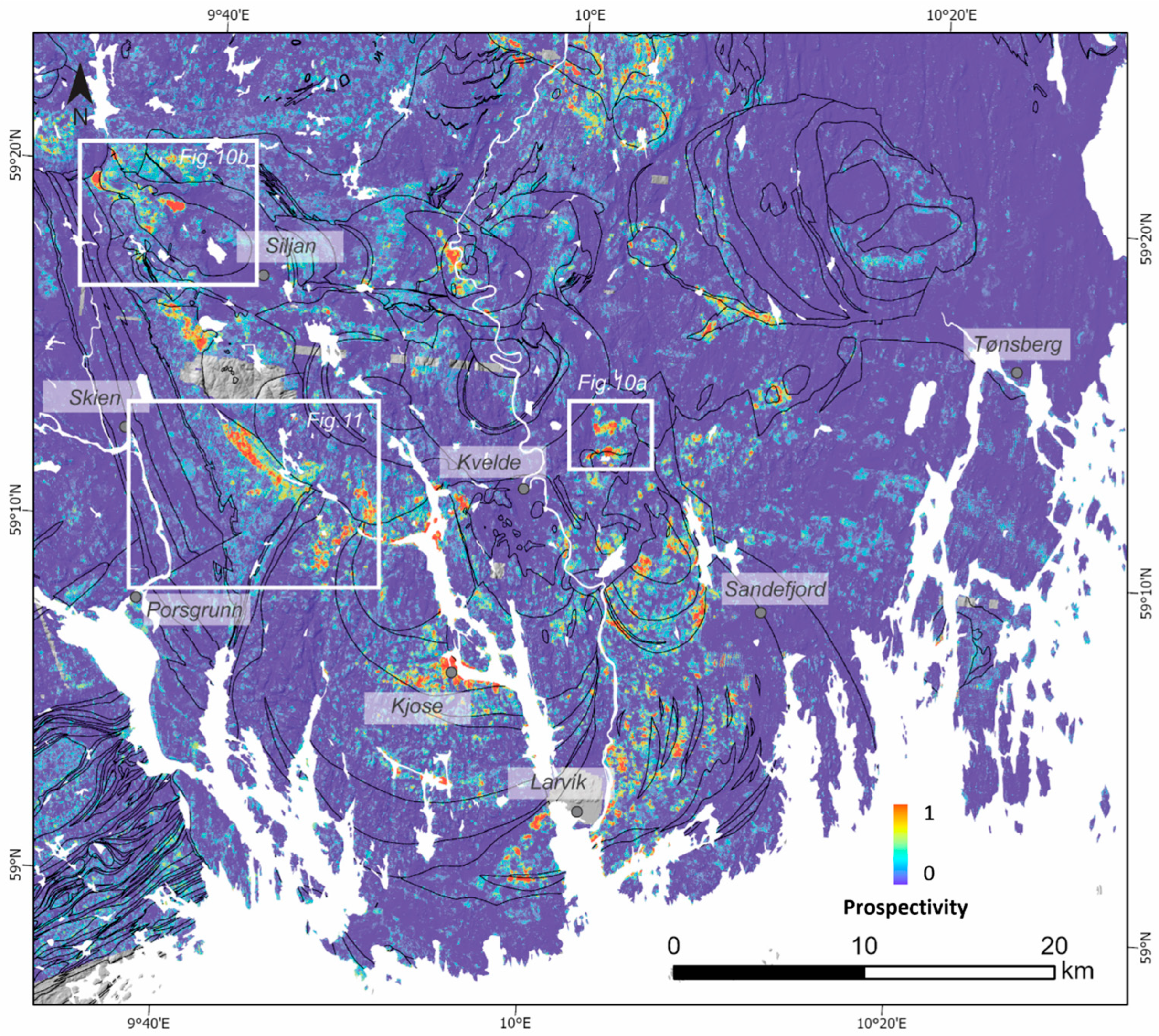
A prospectivity map for the target mineralization (indicated by elevated P2O5 concentrations) was generated for the study region using the trained RF model (Section 4.4) on the 12 feature maps (Section 4.2 and Section 4.3) and is shown in Figure 9. The map region contains 2,668,931 grid cells of size 50 m × 50 m. Each grid cell, referred to as a sample, is associated with a 12-dimentional feature vector and was classified by the trained RF model. Instead of using the predicted binary classes (mineralized or non-mineralized) directly for each sample, we opted to output the predicted probabilities of the sample belonging to the mineralized class. This probability measures the model’s confidence in its predictions regarding whether a sample belongs to the mineralized class and therefore reflects the prospectivity of hosting the target mineralization.
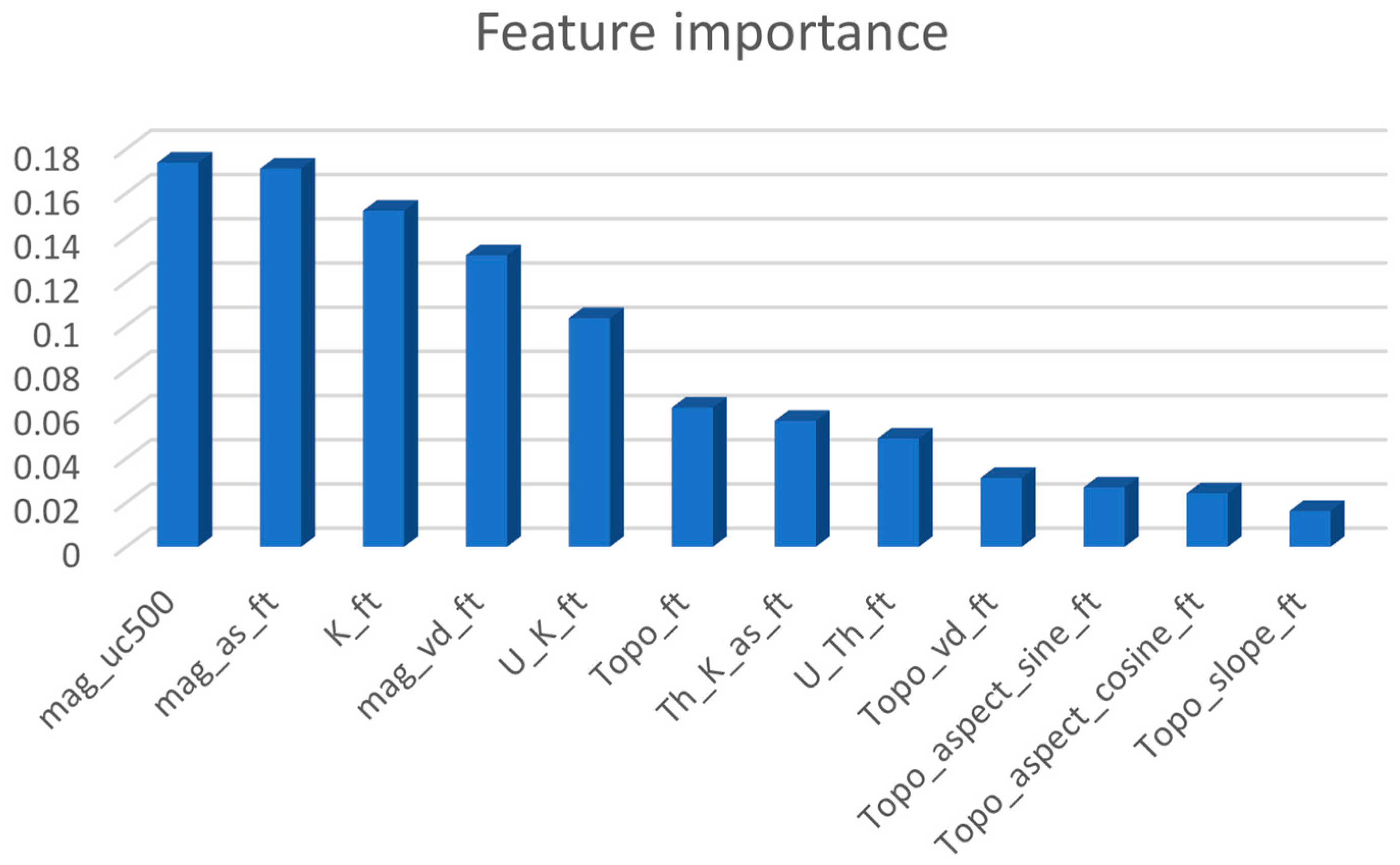
Permutation feature importances [19] are computed to assess the importance of features in the trained RF model. These importances are quantified by assessing how much the model’s prediction error increases when the values of a particular predictor are randomly shuffled or permuted. In Figure 10, we show the feature importances in descending order, highlighting the most influential predictors. In general, the magnetic features and potassium (K) are the most important predictors for our model, while the topographic features are less influential. This is consistent with the domain knowledge described in Section 2.
Several areas are highlighted as highly prospective (yellow to red) for Fe-Ti-P-REE mineralization in Figure 9, and they make up about 0.3% of the entire region. In the following sections, we assess the validity of the prediction at three selected areas based on local geological knowledge and observations in the field.

5.1. Area 1 of 3: Kodal

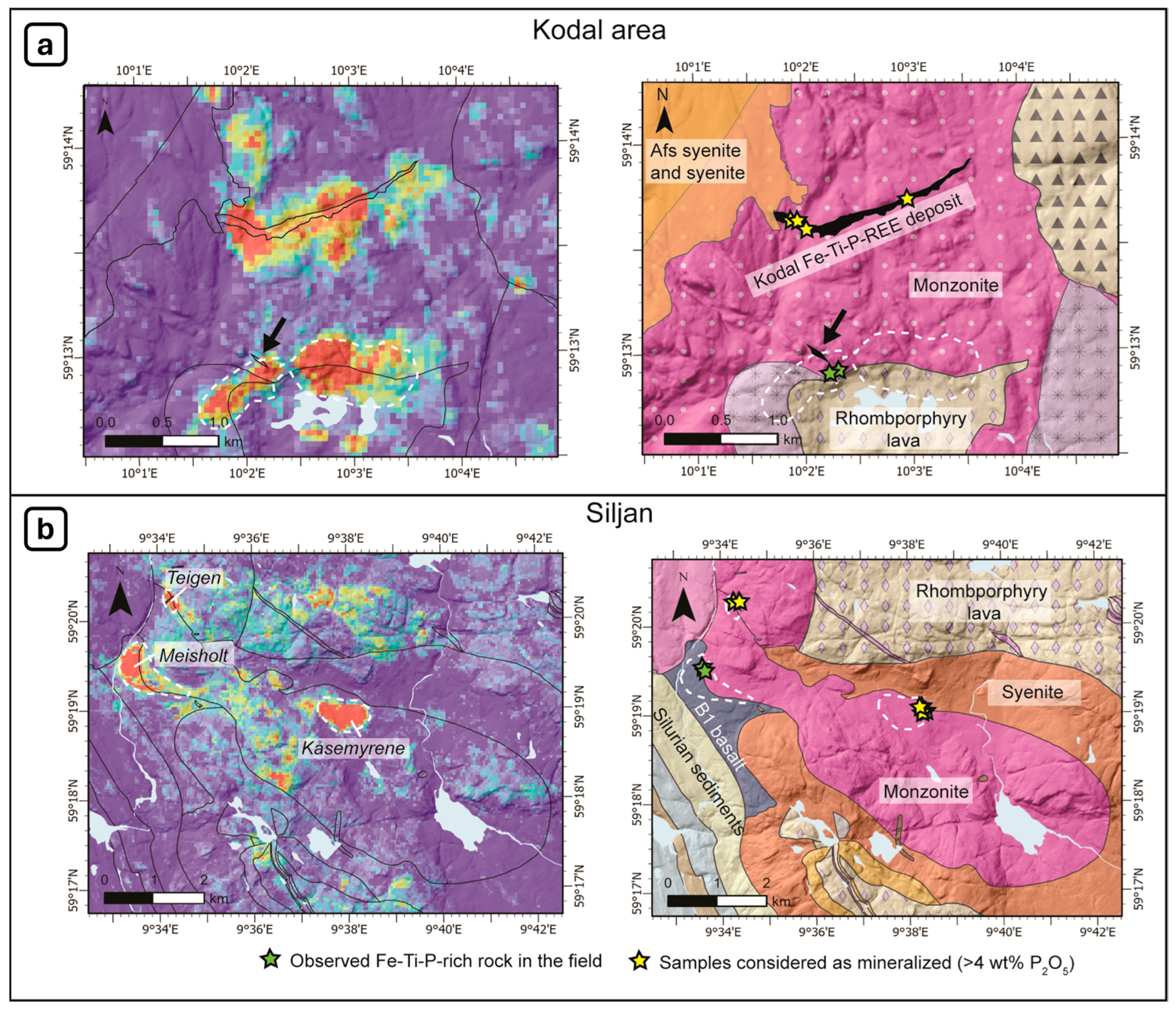
As mentioned in Section 2, Kodal constitutes the largest known Fe-Ti-P-REE deposit in the study region. Our prospectivity map shows a continuation of the deposit between the two sampled areas where mineralization has been observed on the ground surface. This finding is supported by previous work [5,30].
In addition to the main anomaly associated with the Kodal ore deposit, we have identified a second promising area directly south and roughly parallel to the known deposit, marked by white dotted enclosures in Figure 11a. Geological mapping conducted by Kodal Minerals [39] led to the discovery of a showing in this area, as indicated by a black arrow in Figure 11a. As part of this study, we conducted field validation in the high-prospective area and found some mineralizations showing at the surface. This alignment between our high-prospectivity prediction and the geological observation reinforces the value of the prospectivity map as a reliable tool for narrowing the target areas. This strengthens the case for conducting more detailed prospection in this area, as it holds the potential for substantial findings during a thorough exploration.

5.2. Area 2 of 3: Siljan

The prospectivity map over the Siljan area shows the identity of three primary regions of interest, outlined by the white dotted enclosures in Figure 11b. Although there is no large known mineralization directly associated with the Siljan intrusion, the presence of several meter-scale excavation sites where massive Fe-Ti-P-REE-rich rocks are outcropping indicates that the conditions for forming mineralization were once attained in this region.
In the Kåsemyrene area (central circled area in Figure 11b), samples can only be retrieved from one location due to the outcrop situation. However, the prospectivity map suggests that the mineralization might extend beyond its currently known extent. This finding is significant, as it could potentially lead to the discovery of a larger ore body in the vicinity.
Regarding Teigen, the high prospectivity is related to the presence of two mineralized samples in the training dataset. However, the map does not predict the existence of larger mineralization in the nearby area. This information is crucial for planning future prospecting campaigns, as it helps us to focus efforts on areas with a higher likelihood of significant findings.
In the Meisholt area (southwest on the map in Figure 11b), a larger region is classified as highly prospective. According to the geological map, part of this area lies within basalts. Previous excavation at the contact between the basalt and syenite confirmed the presence of mineralized rocks, although they exhibit a low content of P, resulting in their exclusion from the classification of mineralized samples. Additional mapping is necessary in this region to accurately assess the location of geological units and determine the nature of the mineralization.

5.3. Area 3 of 3: Contact between B1-Basalt and Monzonite/Syenites

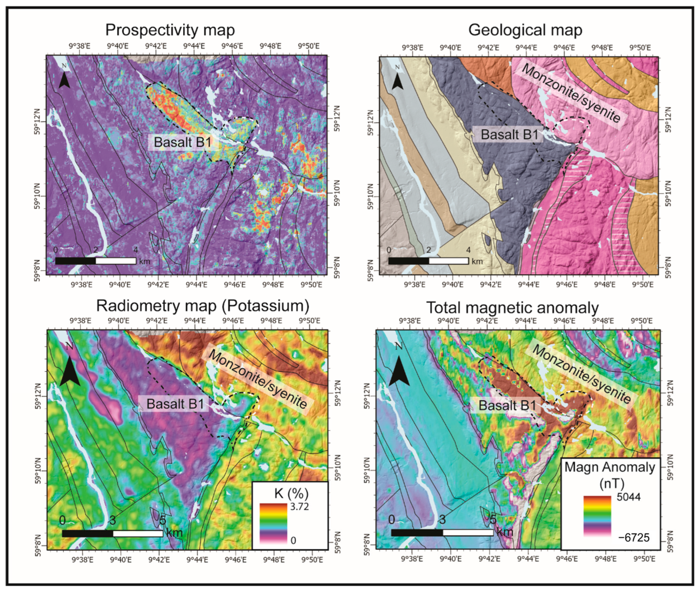
The areas being predicted with a high prospectivity are, however, not all as promising as those in Kodal and Siljan. Figure 12 shows the largest predicted prospective area for Fe-Ti-P-REE mineralization in our prospectivity map, outlined by a black dotted enclosure. The area is dominated by basalt and not monzonite or syenite. Although basalt was emplaced during Permian rifting in the region, Fe-Ti-P-REE mineralization is not associated with this lithology. There are two possible explanations for this area being labelled as prospective. The first one is that the location of the boundary between the basalt and monzonite/syenite on the geological map is not accurate. Although geological boundaries can sometimes be imprecise due to varying mapping quality, it is improbable that the issue lies solely in the mapping quality in this case. Basalt is a rock type that is depleted in potassium (K) compared to the surrounding rock types and especially the monzonite and syenites hosting the targeted mineralization. A regional radiometric survey for potassium shows that the basalt polygon on the geologic map fits well with the radiometric data, with the exception of a small area where low K values appear to be located in the syenite. The second possibility is that basalt is mistaken for the Fe-Ti-P-REE mineralization by the model. Because basalt has some similar petrophysical (highly magnetic) and geochemical (low K) properties as the mineralization we are targeting in our study and these parameters play an important role in the construction of the prospectivity map (the feature importance analysis in Figure 10), part of the basalt areas were classified as having potential mineralization. This highlights the importance of using the available geological information to support the interpretation of predictive maps.
The area with a lower prospectivity, indicated by the white dotted enclosure, is nonetheless interesting. It is located in the syenite and monzonite rock types. The radiometry results show that while potassium does not have a clear signature of the basalt, the area does not contain as much potassium as the surrounding monzonite and syenite. The strong magnetic anomaly is related to pegmatitic syenites containing large crystals of magnetite. These pegmatitic rocks contain little phosphorous but have a relatively high concentration of REEs, indicating that the prospectivity map also contains information that could highlight mineralizations that are not exactly the targeted ones but have similar properties. This is comparable to the case of Meisholt in Siljan, where the P2O5 concentration does not reach 4 wt.% (Section 5.2).
To summarize, a broad evaluation of our resulting prospectivity map and a detailed investigation of a few selected areas (examples described in Section 5.1, Section 5.2 and Section 5.3) support its merit, despite some acknowledged limitations. The machine learning methods used in this context heavily rely on measured data, particularly surficial signatures, and their association with observed mineralization. However, mineralization results from complex processes, requiring in-depth investigation to gain a detailed understanding. Nevertheless, applying machine learning methods to the available high-spatial-resolution maps efficiently provides valuable insights to guide further investigation. Specifically, mineral exploration in the study area is challenging due to the extensive vegetation cover, making field visits difficult. Geophysical data are cost-effective in terms of capturing large-scale spatial variations in a short time. For this project, we benefited from these already available data to offer a first-order prediction of the study region’s mineral potential for an effective initial exploration.
Looking ahead, we aim to enhance our mineral potential mapping efforts by incorporating other data types such as soil geochemistry, which are to be acquired as the project progresses. It is also possible to refine the sampling strategy for field data collection, taking into account the imbalanced dataset issue highlighted in the study. It is worth noting that the currently available samples are superior to many other data-driven mineral potential mapping cases, as they include confirmed negative samples and exhibit a broad spatial distribution across various geological units rather than being limited to only ‘interesting’ locations.
Additionally, we may consider relaxing the constraints on the training dataset preparation to allow for more optimistic predictions. Although the 50 m resolution in our spatial data is relatively high compared to the field sampling resolution typically collected by geologists, the target size of the mineralization varies significantly, ranging from less than a meter to a few hundred meters. As part of our future work, we will investigate how these differences in data resolution and target scale might impact the detectability of the machine learning models.
Therefore, for successful mineral prospectivity mapping using machine learning, one must be aware of the data-driven nature of the methods and emphasize a solid geological understanding. Thoroughly evaluating relevant properties in the available datasets and expertly interpreting predictive maps are vital. Equally critical is the skillful handling of data to create informative features that significantly impact the accuracy of predictions. By combining these factors, it is possible to make more informed decisions and gain valuable insights to effectively guide mineral exploration efforts.

6. Conclusions

Our study addresses the rising global demand for critical raw materials, focusing on the Southern Oslo Rift region in Norway. We successfully generated a prospectivity map for Fe-Ti-P-REE mineralization by training a machine learning model on high-resolution geophysical and topographical data. Whole-rock geochemical analyses of field samples were integrated to construct our training dataset, and our workflow was conducted with rigor, incorporating domain expertise whenever possible. Our approach contributes to advancing the field of mineral prospecting, presenting a practical framework for early-stage exploration efforts. The predictive model effectively narrows down regions for further investigation, offering valuable guidance for mineral exploration in the Oslo Rift region.

Supplementary Materials

The following supporting information can be downloaded at: https://www.mdpi.com/article/10.3390/min14040377/s1, Figure S1: the receiver operating characteristic (ROC) curve of the random forest classification model. The ROC curve illustrates the performance of the model by presenting the trade-off between its true-positive rate and false-positive rate across various classification thresholds. It provides valuable insights into the model’s ability to discriminate between different classes, with a higher area under the curve (AUC) generally indicating a superior discriminatory performance.

Author Contributions

Conceptualization, N.C., Y.W. and E.T.M.; methodology, Y.W., N.C. and E.T.M.; formal analysis, Y.W., N.C. and E.T.M.; data curation, N.C., A.N. and V.C.B.; writing—original draft preparation, Y.W., N.C. and E.T.M.; writing—review and editing, P.A.-G., A.C.R.M., A.N. and V.C.B.; visualization, Y.W. and N.C.; fieldwork, N.C., E.T.M., A.C.R.M. and P.A.-G.; project administration, N.C.; funding acquisition, N.C. All authors have read and agreed to the published version of the manuscript.

Funding

This research was co-funded by the Geological Survey of Norway (NGU) and Treschow-Fritzøe.

Data Availability Statement

In Section 3, the authors have provided links to publicly available datasets that have contributed to this study. However, for the geochemistry analysis of the rock samples, interested parties should make a formal request to the Geological Survey of Norway (NGU), the custodian of the data.

Acknowledgments

We are grateful to our colleagues at the Geological Survey of Norway (NGU) laboratory for their assistance with the chemical analysis of the rock samples. We would also like to thank NGU and Treschow-Fritzøe for co-funding this project.

Conflicts of Interest

The authors declare no conflicts of interest.

References

  1. Blengini, G.A.; Nuss, P.; Dewulf, J.; Nita, V.; Peirò, L.T.; Vidal-Legaz, B.; Ciupagea, C.; Mancini, L.; Blagoeva, D.; Pennington, D.; et al. EU methodology for critical raw materials assessment: Policy needs and proposed solutions for incremental improvements. Resour. Policy 2017, 53, 12–19. [Google Scholar] [CrossRef]
  2. McNulty, B.A.; Jowitt, S.M. Barriers to and uncertainties in understanding and quantifying global critical mineral and element supply. Science 2021, 24, 102809. [Google Scholar] [CrossRef] [PubMed]
  3. EU Regulation Proposal. Regulation of the European Parliament and of the Council Establishing a Framework for ENSURING a secure and Sustainable Supply of Critical Raw Materials and Amending Regulations (EU) 168/2013, (EU) 2018/858, 2018/1724 and (EU) 2019/1020. Brussels 2023, Annex II, 16p. Available online: https://eur-lex.europa.eu/legal-content/EN/ALL/?uri=CELEX:52023PC0160 (accessed on 20 March 2023).
  4. Decrée, S.; Coint, N.; Debaille, V.; Hagen-Peter, G.; Leduc, T.; Schiellerup, H. The Potential for REEs in Igneous-related Apatite Deposits in Europe. In Geological Society; Special Publications: London, UK, 2022; Volume 526. [Google Scholar]
  5. Ihlen, P.M.; Schiellerup, H.; Gautneb, H.; Skår, Ø. Characterization of apatite resources in Norway and their REE potential—A review. Ore Geol. Rev. 2014, 58, 126–147. [Google Scholar] [CrossRef]
  6. Coint, N.; Mansur, E.; Keiding, J.K.; Skår, Ø. Trace elements in ilmenite, titanomagnetite and apatite unravel the petrogenesis of Fe-Ti-P (+/-Zr) rich rocks and associated nelsonite from the Raftsund intrusion, Vesterålen-Lofoten AMCG suite, Northern Norway. Lithos 2023, 460, 107389. [Google Scholar] [CrossRef]
  7. Kodal Minerals plc. Group Annual Report and Financial Statements for the Year Ended 31 March 2014; Kodal Minerals plc: London, UK, 2014; 55p. [Google Scholar]
  8. Zuo, R.G.; Carranza, E.J.M. Support vector machine: A tool for mapping mineral prospectivity. Comput. Geosci. 2011, 37, 1967–1975. [Google Scholar] [CrossRef]
  9. Harris, J.R.; Grunsky, E.C. Predictive lithological mapping of Canada’s North using Random Forest classification applied to geophysical and geochemical data. Comput. Geosci. 2015, 80, 9–25. [Google Scholar] [CrossRef]
  10. Carranza, E.J.M.; Laborte, A.G. Data-driven predictive mapping of gold prospectivity, Baguio district, Philippines: Application of Random Forests algorithm. Ore Geol. Rev. 2015, 71, 777–787. [Google Scholar] [CrossRef]
  11. Zuo, R.G.; Xiong, Y.H.; Wang, J.; Carranza, E.J.M. Deep learning and its application in geochemical mapping. Earth-Sci. Rev. 2019, 192, 1–14. [Google Scholar] [CrossRef]
  12. Chudasama, B.; Torppa, J.; Nykänen, V.; Kinnunen, J.; Lerssi, J.; Salmirinne, H. Target-scale prospectivity modeling for gold mineralization within the Rajapalot Au-Co project area in northern Fennoscandian Shield, Finland. Part 1: Application of knowledge-driven- and machine learning-based-hybrid- expert systems for exploration targeting and addressing model-based uncertainties. Ore Geol. Rev. 2022, 147, 104937. [Google Scholar]
  13. Liu, H.; Harris, J.; Sherlock, R.; Behnia, P.; Grunsky, E.; Naghizadeh, M.; Rubingh, K.; Tuba, G.; Roots, E.; Hill, G. Mineral prospectivity mapping using machine learning techniques for gold exploration in the Larder Lake area, Ontario, Canada. J. Geochem. Explor. 2023, 253, 107279. [Google Scholar] [CrossRef]
  14. Harris, J.R.; Naghizadeh, M.; Behnia, P.; Mathieu, L. Data-driven gold potential maps for the Chibougamau area, Abitibi greenstone belt, Canada. Ore Geol. Rev. 2022, 150, 105176. [Google Scholar] [CrossRef]
  15. Wang, L.J.; Peeters, L.; MacKie, E.J.; Yin, Z.; Caers, J. Unraveling the uncertainty of geological interfaces through data-knowledge-driven trend surface analayis. Comput. Geosci. 2023, 178, 105419. [Google Scholar] [CrossRef]
  16. Jiang, L.; Li, C.; Cai, Z.; Zhang, H. Sampled Bayesian Network Classifiers for Class-Imbalance and Cost-Sensitive Learning. In Proceedings of the IEEE 25th International Conference on Tools with Artificial Intelligence, Herndon, VA, USA, 4–6 November 2013; pp. 512–517. [Google Scholar]
  17. Juliani, C.J.; Ellefmo, S.L. Prospectivity Mapping of Mineral Deposits in Northern Norway Using Radial Basis Function Neural Networks. Minerals 2019, 9, 131. [Google Scholar] [CrossRef]
  18. Prado, E.M.G.; de Souza Filho, C.R.; Carranza, E.J.M.; Motta, J.G. Modeling of Cu-Au prospectivity in the Carajás mineral province (Brazil) through machine learning: Dealing with imbalanced training data. Ore Geol. Rev. 2020, 124, 103611. [Google Scholar] [CrossRef]
  19. Breiman, L. Random forests. Mach. Learn. 2001, 45, 5–32. [Google Scholar] [CrossRef]
  20. Cortes, C.; Vapnik, V. Support-vector networks. Mach. Learn. 1995, 20, 273–297. [Google Scholar] [CrossRef]
  21. Neumann, E.R.; Wilson, M.; Heeremans, M.; Ann Spencer, E.; Obst, K.; Timmerman, M.J.; Kirstein, L. Carboniferous-Permian rifting and magmatism in southern Scandinavia, the North Sea and northern Germany: A review. Geol. Soc. Lond. Spec. Publ. 2004, 223, 11–40. [Google Scholar] [CrossRef]
  22. Ziegler, P.A.; Schumacher, M.E.; Dèzes, P.; Van Wees, J.-D.; Cloetingh, S. Post-Variscan evolution of the lithosphere in the area of the European Cenozoic Rift System. Geol. Soc. Lond. Mem. 2006, 32, 97–112. [Google Scholar] [CrossRef]
  23. Larsen, B.T.; Olaussen, S.; Sundvoll, B.; Heeremans, M. The Permo-Carboniferous Oslo Rift through six stages and 65 million years. Episodes 2008, 31, 52–58. [Google Scholar] [CrossRef]
  24. Rämö, O.T.; Andersen, T.; Whitehouse, M.J. Timing and Petrogenesis of the Permo-Carboniferous Larvik Plutonic Complex, Oslo Rift, Norway: New Insights from U–Pb, Lu-Hf, and O Isotopes in Zircon. J. Petrol. 2022, 63, egac116. [Google Scholar] [CrossRef]
  25. Neumann, E.R.; Dunworth, E.A.; Sundvoll, B.A.; Tollefsrud, J.I. B1 basaltic lavas in Vestfold–Jeløya area, central Oslo rift: Derivation from initial melts formed by progressive partial melting of an enriched mantle source. Lithos 2002, 61, 21–53. [Google Scholar] [CrossRef]
  26. Pedersen, L.E.; Heaman, L.M.; Holm, P.M. Further Constraints on the Temporal Evolution of the Oslo Rift from Precise U-Pb Zircon Dating in the Siljan-Skrim Area. Lithos 1995, 34, 301–315. [Google Scholar] [CrossRef]
  27. Lindberg, P.A. Fe-Ti-P Mineralizations in the Larvikite-Lardalite Complex, Oslo Rift. NGU Bull. 1985, 402, 93–98. [Google Scholar]
  28. Andersen, T.E. Immiscibility as a Rock Forming Process in Shallowly Emplaced Alkalic Metaluminous Granitoids. Master’s Thesis, NTNU, Trondheim, Norway, 2021. [Google Scholar]
  29. Andersen, T.; Seiersten, M. Deep cumulates in a shallow intrusion- origin and crystallization history of a pyroxenite (jacupirangite SL) body in the Larvik pluton, Oslo Region, South Norway. Neues Jahrb. Mineral.-Monatshefte 1994, 1994, 255–274. [Google Scholar]
  30. Bergstøl, S. The jacupirangite at Kodal, Vestfold, Norway. Miner. Depos. 1972, 7, 233–246. [Google Scholar] [CrossRef]
  31. Baranwal, V.C. Compilation of Various Airborne Geophysical Data in the Oslofjord Area. NGU Report 2013.030. 2016. Available online: https://hdl.handle.net/11250/2664326 (accessed on 20 March 2023).
  32. Coint, N.; Keiding, J.K.; Ihlen, P.M. Evidence for silicate–liquid immiscibility in monzonites and petrogenesis of associated Fe–Ti–P-rich rocks: Example from the Raftsund Intrusion, Lofoten, Northern Norway. J. Petrol. 2020, 61, egaa045. [Google Scholar] [CrossRef]
  33. He, H.; Garcia, E.A. Learning from Imbalanced Data. IEEE Trans. Knowl. Data Eng. 2009, 21, 1263–1284. [Google Scholar]
  34. Prati, R.C.; Batista, G.E.A.P.A.; Silva, D.F. Class imbalance revisited: A new experimental setup to assess the performance of treatment methods. Knowl. Inf. Syst. 2015, 45, 247–270. [Google Scholar] [CrossRef]
  35. Blakely, R.J. Potential Theory in Gravity and Magnetic Applications; Cambridge University Press: Cambridge, UK, 1996. [Google Scholar]
  36. Lentz, D. Radioelement distribution in U, Th, Mo, and rare-earth-element pegmatites, skarns, and veins in a portion of the Grenville Province, Ontario and Quebec. Can. J. Earth Sci. 1991, 28, 1–12. [Google Scholar] [CrossRef]
  37. Dentith, M.C.; Mudge, S.T. Geophysics for the Mineral Exploration Geoscientist; Cambridge University Press: Cambridge, UK, 2014. [Google Scholar]
  38. Guyon, I.; Elisseeff, A. An introduction to variable and feature selection. J. Mach. Learn. Res. 2003, 3, 1157–1182. [Google Scholar]
  39. Kodal Minerals plc. Kodal Project Exploration Report-2016; Kodal Minerals plc: London, UK, 2016; 22p. [Google Scholar]
Figure 1. (a) The location of the study area in Norway; (b) simplified geologic map of the study area based on the 1:250,000 harmonized bedrock map of Norway which is published and maintained by Geological Survey of Norway; (c) the Kodal deposit.
Minerals 14 00377 g001
Figure 2. Examples of mineralization in rocks where the training samples were collected and analyzed. (a,b) Fe-Ti-P-REE mineralization from the Kodal ore deposit; (c,d) Fe-Ti-P-REE mineralization associated with the Siljan-Hværnes intrusions (SHI); (e) Fe-Ti-P-REE mineralization in Kjose (LPC).
Minerals 14 00377 g002
Figure 3. The high-resolution geospatial datasets projected onto a uniform grid with a 50 m cell size: (a) the total magnetic field anomaly (nT); (b) potassium (K) concentration (%); (c) topography (DEM) (m); (d) geography map to indicate the data coverage which is beyond the study region shown in Figure 1. Field sample locations are marked in (ac) and differentiated using red dots to indicate mineralized samples and black dots to indicate non-mineralized samples.
Minerals 14 00377 g003
Figure 4. Illustration of the training data sampling strategy. The true locations of the non-mineralized (i.e., negative) and mineralized (i.e., positive) field samples are indicated by black dots and red circles, respectively. The green and magenta pointers correspond to the uniform grid (with a 50 m cell size) onto which the high-resolution spatial datasets are projected. Specifically, all the green pointers are located within a 50 m distance from at least one non-mineralized field sample (a); whereas all the magenta pointers are located within a 100 m from at least one mineralized sample (b); in cases of overlapping grid cells, the positive samples overrule the negative samples, as shown in (c).
Minerals 14 00377 g004
Figure 5. Predictive features corresponding to the airborne magnetic data. (a) mag_ft; (b) mag_as_ft; (c) mag_uc500; (d) mag_vd_ft; (e) mag_tdr. The color bars associated with the feature plots indicate the relative data range and strength, but no physical units are provided. This is because the feature engineering process may have changed the scale or range of the original data, rendering the physical units no longer meaningful.
Minerals 14 00377 g005
Figure 6. Predictive features corresponding to the airborne radiometric data. (a) K_ft; (b) Th_ft; (c) U_ft; (d) Th_K_as_ft; (e) U_K_ft; (f) U_Th_ft. The color bars associated with the feature plots indicate the relative data range and strength, but no physical units are provided. This is because the feature engineering process may have changed the scale or range of the original data, rendering the physical units no longer meaningful.
Minerals 14 00377 g006
Figure 7. Predictive features corresponding to the topographic data. (a) Topo_ft; (b) Topo_vd_ft; (c) Topo_slope_ft; (d) Topo_aspect_sine_ft; (e) Topo_aspect_cosine_ft. The color bars associated with the feature plots indicate the relative data range and strength, but no physical units are provided. This is because the feature engineering process may have changed the scale or range of the original data, rendering the physical units no longer meaningful.
Minerals 14 00377 g007
Figure 8. Correlation matrix among 16 candidate features including 5 magnetic features, 6 radiometric features, and 5 topographic features. The correlation coefficients range from −1 to +1, where −1 indicates a 100% negative correlation, +1 indicates a 100% positive correlation, and a value of 0 indicates no correlation.
Minerals 14 00377 g008
Figure 9. Prospectivity map of the target mineralization generated using the RF classification model. The prospectivity measure is defined by the predicted probability of a sample belonging to the positive (mineralization) class. Water bodies are masked away. The three white bounding boxes mark the three areas for detailed discussion.
Minerals 14 00377 g009
Figure 10. Feature importance for the RF model. Predictor abbreviations are explained in Section 4.2.
Minerals 14 00377 g010
Figure 11. Comparison between the prospectivity map (on the left) and the geology map (on the right) at (a) Kodal and (b) Siljan. The yellow stars mark the locations of the samples considered to be mineralized, which were used as positive training samples in this study. The green stars mark the locations where Fe-Ti-P-rich rocks were observed during field validation.
Minerals 14 00377 g011
Figure 12. Comparison of the prospectivity map at the vicinity of the B1-basalt with the geology map, potassium (K) map, and total magnetic anomaly map.
Minerals 14 00377 g012
Disclaimer/Publisher’s Note: The statements, opinions and data contained in all publications are solely those of the individual author(s) and contributor(s) and not of MDPI and/or the editor(s). MDPI and/or the editor(s) disclaim responsibility for any injury to people or property resulting from any ideas, methods, instructions or products referred to in the content.