Modeling and Hybrid Inversion of Mineral Deposits Using the Dipping Dike Model with Finite Depth Extent

Abstract

The dipping dike model has shown to be a useful approximation for mineral deposits. To make this model more realistic, we include the thickness, which yields the depth to the bottom, as an additional parameter. The magnetic anomaly is obtained by combining the anomalies of two infinite dikes, so that the resulting expression is simpler than the classical prismatic models with polygonal cross section. We employ a Metropolis-Hasting (MH) algorithm coupled with the Levenberg-Marquardt (LM) method to invert magnetic profiles assuming a model of multiple dike-like sources. We use a few iterations of the LM method to improve the candidate solutions at the end of each random walk generated by MH. The following parameters are obtained: depth to the top, thickness, half-width, horizontal location of the top center, geological dip, in addition to two effective parameters that depend on the intensity of magnetization and the directions of the induced and remanent fields. For synthetic anomalies, both noise-free and noisy magnetic data are considered, with examples presented for each scenario. These examples highlight the discrepancy between models with finite and infinite sources. They also illustrate the higher accuracy of the hybrid MH-LM method over the pure MH approach. Moreover, two field examples related to mineral exploration have been considered: the Pima copper mine, United States, where the relative differences between the parameters obtained by our algorithm and those known from drilling are not higher than 10%, and a magnetic profile over iron ore deposits located in Laje, northeast Brazil, where the inverted parameters were useful for detailing previous studies.

1. Introduction

Magnetometry has been a widely used geophysical method for analyzing and modeling subsurface structures. Magnetic anomalies are particularly useful in the study of magmatic dikes. In this case, the inversion of magnetic data can be based on the dipping dike model [1] to estimate parameters such as depth, width, center, and effective dip angle [2]. The dipping dike model is valuable for interpreting dike-like ore deposits [3,4,5,6].

Local optimization techniques such as Gauss-Newton [7,8] and Levenberg-Marquardt (LM) method [9,10,11] have been widely used to evaluate gravity and magnetic data. However, they require initial model parameters sufficiently close to the true model to avoid convergence to a local minimum. Global optimization methods are usually based on a random search of admissible parameters, making them less susceptible to convergence to local minima and less computationally demanding, as the sensitivity matrix is not required. On the other hand, their convergence rate is slow and some heuristic strategy is usually employed to improve performance, such as simulated annealing [5,12] and evolutionary algorithms, such as genetic algorithm [13], particle swarm optimization [14,15], differential evolution [16], barnacles mating optimization [17], and hunger games search [6,18].

Another global optimization approach is to use Markov Chain Monte Carlo methods [19,20,21], where the geophysical model parameters are estimated from a Bayesian structure. One of their simplest versions is the Metropolis-Hasting (MH) algorithm [22]. These methods are based on the premise of a priori knowledge from a stationary distribution that generates realizations from the current state of the Markov chain to a new state. Inverse problem solutions are derived from a priori information extracted from data and the physics of the problem, which provide posterior probabilities in the model space [16,23].

To benefit from the advantages of local and global optimization techniques, we propose using a hybrid inversion method that combines both approaches [24,25]. We employ the MH algorithm coupled with the LM method to perform the inversion of magnetic anomalies by multiple dike-like sources [5] that are defined not only by their depths to the top, but also by depths to the bottom, i.e., the sources have a finite thickness. We do not assume that the depth extent of the sources is much larger than their width and depth to the top, which is generally true for magmatic dikes but may be too restrictive for dike-like mineral deposits. Rather than using the more complex prismatic models [9,26], we compute the anomaly of a finite dike-like source as the difference of anomalies from two infinite sources, where the deeper one is shifted to account for the geological dip [11]. This approach renders the model more general than the vertical dike with finite depth [25]. In fact, the dipping dike model with finite depth extent can represent prismatic bodies that are not necessarily dike-like sources. For a comprehensive sampling of the search space, we employ multiple Markov chains [27]. However, the number of chains is subject to stopping criteria rather than being fixed. The same applies to the length of each chain. To demonstrate the effectiveness of the proposed inversion method, we applied it to synthetic models with and without random noise, as well as a ground survey data from Pima copper mine in Arizona, USA [28] and iron ore deposits located in Laje, northeast Brazil [29].

2. Method

In the following we describe the dipping-dike model modified from [11] and our hybrid inversion technique based on the MH and LM methods.

2.1. Forward Modeling

The building block of our magnetic anomaly model is based on the classical dipping dike equation [1,30]:

$$\begin{array}{cc}\hfill \Delta \mathbb{T}(x,\alpha ,\theta ,h,K,\overline{x},d)& =Ksin\left(\theta \right)\left[sin\left(\alpha \right)\left({tan}^{-1}{\displaystyle \frac{x-\overline{x}+d}{h}}-{tan}^{-1}{\displaystyle \frac{x-\overline{x}-d}{h}}\right)\right.\hfill \\ & -\left.{\displaystyle \frac{1}{2}}cos\left(\alpha \right)ln\left({\displaystyle \frac{{(x-\overline{x}+d)}^2+h^2}{{(x-\overline{x}-d)}^2+h^2}}\right)\right],\hfill \end{array}$$

(1)

where $\alpha$ is the effective dip angle, h is the depth from the plane of observation to the top of the dike, K is the amplitude coefficient, $\overline{x}$ is the dike center, and d is the half-width. The x-axis is perpendicular to the center line of the dike. The amplitude and the effective dip angle depend on the magnetization intensity J, the geologic dip angle $\theta$, the inclinations $\{I,i\}$ of the Earth’s magnetic field and the resultant magnetization, and the angles $\{A,a\}$ between the positive x axis and the horizontal projection of the Earth’s magnetic field and the resultant magnetization. They are defined as follows:

$$K=2Jbc,b=\sqrt{{sin}^2\left(i\right)+{cos}^2\left(i\right){cos}^2\left(a\right)},c=\sqrt{{sin}^2\left(I\right)+{cos}^2\left(I\right){cos}^2\left(A\right)},$$

(2)

$$\alpha =\lambda +\psi -\theta ,\lambda ={tan}^{-1}{\displaystyle \frac{tan\left(I\right)}{cos\left(A\right)}},\psi ={tan}^{-1}{\displaystyle \frac{tan\left(i\right)}{cos\left(a\right)}}.$$

(3)

The anomaly defined by Equation (1) assumes an infinite depth extent. To account for a finite depth to the bottom H, we consider the difference between the anomalies of two infinite dikes [11]:

$$\Delta T(x,\alpha ,\theta ,h,H,K,\overline{x},d)=\Delta \mathbb{T}(x,\alpha ,\theta ,h,K,\overline{x},d)-\Delta \mathbb{T}(x,\alpha ,\theta ,H,K,{\overline{x}}^{\prime },d),$$

(4)

where the center ${\overline{x}}^{\prime }$ of the deeper dike is given as

$${\overline{x}}^{\prime }=\overline{x}+(H-h)cot\left(\theta \right).$$

(5)

Finally, the magnetic anomaly generated by a superposition of $n_d$ sources is

$$\Delta T=\sum _{i=1}^{n_d}\Delta T(x,{\alpha }_i,{\theta }_i,h_i,H_i,K_i,{\overline{x}}_i,d_i).$$

(6)

We introduce auxiliary variables to reduce the dependence between some parameters. As the effective dip angle ${\alpha }_i$ depends on the geologic dip ${\theta }_i$, we introduce the auxiliary angle

$${\beta }_i={\lambda }_i+{\psi }_i,$$

(7)

which may be unknown due to lack of information about the magnetic remanence or the strike of the sources, thus we regard it as a parameter. Moreover, as $H_i$ depends on $h_i$, we introduce the thickness $t_i=H_i-h_i$. By introducing the parameter vector

$$\mathbf{m}=[{\beta }_1,{\theta }_1,h_1,t_1,K_1,{\overline{x}}_1,d_1,\dots ,{\beta }_{n_d},{\theta }_{n_d},h_{n_d},t_{n_d},K_{n_d},{\overline{x}}_{n_d},d_{n_d}]$$

(8)

of length $n_{par}=7n_d$, our forward-modeling operator is

$$F(x,\mathbf{m})=\sum _{i=1}^{n_d}\Delta T(x,{\beta }_i-{\theta }_i,{\theta }_i,h_i,h_i+t_i,K_i,{\overline{x}}_i,d_i).$$

(9)

2.2. Inversion Algorithm

Let ${\mathbf{F}}_{obs}={[f_1,\dots ,f_{n_{obs}}]}^T$ be a vector containing the magnetic anomaly measurements along a profile at positions $x=x_j$$(1\le j\le n_{obs})$. Our goal is to find the parameter vector $\mathbf{m}$ that minimizes the misfit between the magnetic measurements ${\mathbf{F}}_{obs}$ and the predicted data $\mathbf{F}\left(\mathbf{m}\right)=[F(x_1,\mathbf{m}),\dots ,F(x_{n_{obs}},\mathbf{m})]$. The misfit is represented by the objective function

$$\mathrm{\Phi }\left(\mathbf{m}\right)={\displaystyle \frac{1}{2}}\parallel {\mathbf{F}}_{obs}{-\mathbf{F}\left(\mathbf{m}\right)\parallel }_2^2,{\parallel \mathbf{v}\parallel }_2={\left(\sum _{j=1}^{n_{obs}}{\left|v_j\right|}^2\right)}^{1/2}.$$

(10)

The model parameters are subject to search intervals [4,5] denoted as follows:

$$m_i^{min}\le m_i\le m_i^{max},1\le i\le n_{par}.$$

(11)

The MH method generates a random walk in the model space where the transition from the current sample ${\mathbf{m}}^{n-1}$ to the next sample ${\mathbf{m}}^n$ is performed so that the distribution of the parameter samples converges to a certain distribution $\pi (·)$. For this purpose we employ the Metropolis algorithm, where a candidate sample ${\mathbf{m}}^c$ is accepted if $\pi \left({\mathbf{m}}^c\right)\ge \pi \left({\mathbf{m}}^{n-1}\right)$, otherwise it may be accepted with probability $\pi \left({\mathbf{m}}^c\right)/\pi \left({\mathbf{m}}^{n-1}\right)$ [31], i.e.,

$$p_{acc}=min\left\{1,{\displaystyle \frac{\pi \left({\mathbf{m}}^c\right)}{\pi \left({\mathbf{m}}^{n-1}\right)}}\right\}=\left\{\begin{array}{cc}\hfill \pi \left({\mathbf{m}}^c\right)/\pi \left({\mathbf{m}}^{n-1}\right),& \pi \left({\mathbf{m}}^{n-1}\right)<\pi \left({\mathbf{m}}^c\right),\hfill \\ \hfill 1,& \pi \left({\mathbf{m}}^{n-1}\right)\ge \pi \left({\mathbf{m}}^c\right),\hfill \end{array}\right.$$

(12)

which can be modeled by a binomial distribution [32]. The distribution $\pi (·)$ is the so-called a posteriori distribution, and it measures the model’s ability to fit the data, as the fitness function of genetic algorithms [22]. We employ a classical Bayesian formulation that can be written as follows [31]:

$$\pi \left(\mathbf{m}\right)=C_1\rho \left(\mathbf{m}\right)L\left(\mathbf{m}\right),$$

(13)

where $C_1$ is a normalization constant, $L\left(\mathbf{m}\right)$ is the likelihood function, and $\rho \left(\mathbf{m}\right)$ represents the prior distribution, which we assumed as a multivariate uniform distribution based on the search intervals, i.e., $\rho \sim U({\mathbf{m}}_i^{min},{\mathbf{m}}_i^{max})$. In this simpler case, the probability ratio in Equation (12) reduces to $L\left({\mathbf{m}}^{\mathbf{c}}\right)/L\left({\mathbf{m}}^{\mathbf{n}-\mathbf{1}}\right)$ [31]. We employ the classical Gaussian likelihood function

$$L\left(\mathbf{m}\right)=C_{2}exp\left(-{\displaystyle \frac{\mathrm{\Phi }\left(\mathbf{m}\right)}{{\sigma }^2}}\right),$$

(14)

where $\sigma$ is a precision parameter [33]. The normalizing constant $C_2$ can be disregarded as it is canceled out in the ratio $L\left({\mathbf{m}}^{\mathbf{c}}\right)/L\left({\mathbf{m}}^{\mathbf{n}-\mathbf{1}}\right)$. The candidate model is defined as in [34]:

$${\mathbf{m}}^c=\left[\mathbf{I}+{(-1)}^{n-1}\tau ·{\mathbf{u}}^{n-1}\right]{\mathbf{m}}^{n-1},{\mathbf{u}}^{n-1}\sim U(\mathbf{0},\mathbf{I}),\tau \in (0,1].$$

(15)

Rather than executing the MH algorithm once, we consider a multiple Markov-chain approach [27]. Each chain starts with a initial sample ${\mathbf{m}}^0$ selected with distribution $\rho (·)$, and subsequent samples are generated as described above, until they converge or reach a maximum number of samples, N. As a convergence criterion, we consider that the number of consecutive samples that are not accepted according to the probability (12) should not exceed $N^{rej}$. The final model of each Markov chain is used as an initial model to the LM method:

$${\mathbf{m}}_{\ast }^{k+1}={\mathbf{m}}_{\ast }^k+{\delta }_k\Delta {\mathbf{m}}^k,k=0,\dots ,n_{LM}-1,$$

(16)

for a small number of iterations $n_{LM}$. The parameter ${\delta }_k$ is the Armijo step size [35,36]. Following [8], the value of ${\delta }_k$ may be reduced to ensure that all entries of ${\mathbf{m}}_{\ast }^{k+1}$ satisfy Equation (11). The vector increment $\Delta {\mathbf{m}}^k$ is obtained by solving the following linear system:

$$({\mathbf{J}}_k^T{\mathbf{J}}_k+{\lambda }_k\mathbf{I})\Delta {\mathbf{m}}^k=-{\mathbf{J}}_k^T[{\mathbf{F}}_{obs}-\mathbf{F}\left({\mathbf{m}}_{\ast }^k\right)],{\mathbf{J}}_k={\displaystyle \frac{\partial \mathbf{F}}{\partial \mathbf{m}}}\left({\mathbf{m}}_{\ast }^k\right),$$

(17)

where ${\lambda }_k={\parallel {\mathbf{F}}_{obs}-\mathbf{F}\left({\mathbf{m}}_{\ast }^k\right)\parallel }_2^2$. The Jacobian matrix ${\mathbf{J}}_k$ is obtained by exact differentiation (Appendix A).

If the model obtained at the end of the LM iterations improves the best objective function value of the previous chains, $\mathrm{\Phi }\left({\mathbf{m}}^{opt}\right)$, the algorithm starts a new chain, unless if the maximum number of chains, $N_c$, is reached. On the other hand, the algorithm ends if $\mathrm{\Phi }\left({\mathbf{m}}^{opt}\right)$ remains unchanged after $N_c^{rej}$ chains, or if a reference misfit ${\mathrm{\Phi }}_{ref}$ is reached. We adopt a reference misfit to avoid overfitting. A flowchart outlining the proposed algorithm is given in Figure 1, and its computer implementation is available in the article’s Supplementary Data.

Although the MH algorithm can be used for uncertainty quantification of the model parameters, the local search step of our hybrid approach could introduce some bias. Hence, MH is regarded only as a global optimization method in our approach [37].

3. Results and Discussion

Our examples are based on synthetic and field magnetic profiles, where we compare the MH algorithm with our proposed hybrid MH-LM version. The MH algorithm is executed with at most $N_c=500$ chains, each with up to $N=$ 500,000 samples, whereas $N_c^{rej}=50$ and $N^{rej}=1000$. These parameters should ensure that even challenging inverse problems, with potentially complex nonlinear relationships, could be handled effectively without premature termination of the optimization process. Following [34,37], we employ the precision and tuning parameters $\sigma =0.3$ and $\tau =0.0025$, respectively. Moreover, we employed the initial Armijo step ${\delta }_k=0.7$ [36].

Although the algorithms were described and implemented using the objective function $\mathrm{\Phi }$ in Equation (10), we will report the misfit in terms of the root-mean-square (RMS) error

$$\mathrm{RMS}=\sqrt{2\mathrm{\Phi }/n_{obs}}.$$

(18)

In the synthetic and field examples that follow, we have not addressed the effect of regional information in the inversion. Regional information could be considered by including a term of the form $Mx+C$ in Equation (9), as in [38], or by a moving average residual approach [6,18,39].

3.1. Synthetic Data

We consider the synthetic example from [40], given by a model of three prismatic sources. They are defined by the parameters provided in

Table 1. Parameters of the synthetic model.

	$\mathit{\beta }{(}^{\circ })$	$\mathit{\theta }{(}^{\circ })$	h (km)	t (km)	K (nT)	$\overline{\mathit{x}}$ (km)	d (km)
Prism 1	180	90	1	4	126	7.5	1.5
Prism 2	180	90	2	2	126	20	5
Prism 3	180	63.4	1	4	126	33.5	2.5

and are outlined in Figure 2a. In this example, $I=i={90}^{\circ }$ and $A=a=0^{\circ }$. The sampling interval is $\Delta x=0.25$ km.

Figure 2 illustrates the effect of depth extent in the magnetic anomaly by comparing the sources defined in [40] with the ones where depth to bottom is infinite. As the anomalies generated by finite and infinite models are significantly different, they might lead to different interpretations of magnetic data. We emphasize that the dipping dike model with finite depth extent, Equation (4), applies not only to dike-like sources, but also some prismatic sources such as those in Figure 2a.

Let us proceed to the hybrid inversion. The search interval for each parameter $m_i$ is $[0.5m_i^{ex},1.5m_i^{ex}]$, i.e., it is centered around the exact parameter value $m_i^{ex}$ with tolerance of ±50%. For instance, the search interval for the angle $\beta$ is $[{90}^{\circ },{270}^{\circ }]$.

We conducted this experiment first with the magnetic anomaly free of noise and then perturbed by Gaussian noise with a standard deviation of 5 nT. The reference misfit ${\mathrm{\Phi }}_{ref}$ is chosen such that RMS error at the noise-free and noisy cases are ${\mathrm{RMS}}_{ref}$ = 0 nT and ${\mathrm{RMS}}_{ref}$ = 5 nT, respectively. The results for both cases are summarized in

Table 2. Number of chains, average chain length, RMS error, and relative error of the MH ($n_{LM}=0$) and MH-LM ($n_{LM}=1,\dots ,8$) methods for the synthetic example with noise-free and noisy data.

	Noise-Free				Noisy
${\mathit{n}}_{\mathit{LM}}$	${\mathit{n}}_{\mathit{c}}$	$\overline{\mathit{n}}$	RMS (nT)	$\overline{\mathit{e}}$ (%)	${\mathit{n}}_{\mathit{c}}$	$\overline{\mathit{n}}$	RMS (nT)	$\overline{\mathit{e}}$ (%)
0	118	285,563	2.942	16.801	80	283,684	6.422	17.062
1	80	258,966	1.984	11.055	114	244,822	5.407	15.164
2	72	243,736	1.366	9.511	64	237,269	6.142	16.610
4	80	246,701	1.081	8.483	50	265,891	4.979	10.879
8	53	244,945	0.299	5.513	13	260,869	4.923	7.434

where, in addition to the RMS error, we show the mean relative error

$$\overline{e}=\sum _{i=1}^{n_{par}}{\displaystyle \frac{|m_i-m_i^{ex}|}{m_i^{ex}}}.$$

(19)

As shown in Table 2, the local LM iterations helped to reduce the number of chains and the average chain length (i.e., the average number of MH iterations within each chain), and led to a decrease in the mean relative error. The total-field anomalies obtained by the MH method and the MH-LM method with $n_{LM}=8$, as well as the corresponding inverted models, are compared with the true anomalies and models in Figure 3 for the noise-free case and Figure 4 for the noisy case. The superiority of the MH-LM approach is confirmed in both cases.

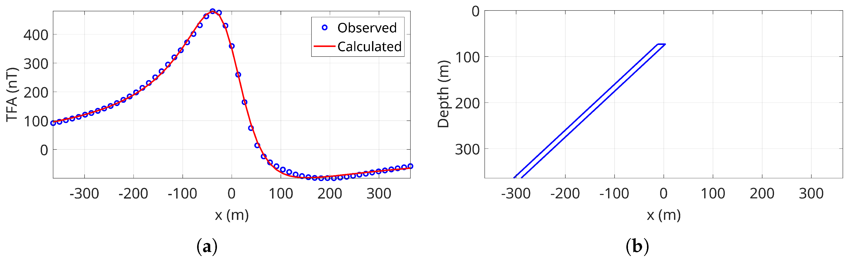
3.2. Pima Copper Mine

In this example, we study a vertical magnetic anomaly profile over the Pima copper mine in Arizona, United States [28]. The Pima copper mine is one of the largest porphyry copper deposits of the nineteenth century, producing significant amounts of copper, molybdenum, lead, silver, and gold [14]. This anomaly profile has become a benchmark with numerous studies in the literature [4,5,12,13,14,38,41,42] especially because some source parameters were provided by drilling [28]:

• Depth: $h=63.7$ m;
• Dip: $\theta ={135}^{\circ }$;
• Half-width: $d=7.54$ m (or $5.33$ m perpendicular to the dip).

Moreover, the Earth’s magnetic field inclination is $I={59}^{\circ }$ and its effective inclination is $\lambda ={62}^{\circ }$ ([28], Figure 10), thus $A={27.75}^{\circ }$.

In this example, we consider a single source, thus we drop the sub-indices i in Equation (9). To account for the vertical component of the magnetic field, we must replace Equation (1) with the following one [1,38]:

$$\begin{array}{cc}\hfill \Delta \mathbb{Z}(x,\alpha ,\theta ,h,K,\overline{x},d)& =2Jbsin\left(\theta \right)\left[cos(\psi -\theta )\left({tan}^{-1}{\displaystyle \frac{x-\overline{x}+d}{h}}-{tan}^{-1}{\displaystyle \frac{x-\overline{x}-d}{h}}\right)\right.\hfill \\ & +\left.{\displaystyle \frac{1}{2}}sin(\psi -\theta )ln\left({\displaystyle \frac{{(x-\overline{x}+d)}^2+h^2}{{(x-\overline{x}-d)}^2+h^2}}\right)\right],\hfill \end{array}$$

(20)

where b and $\psi$ are defined in Equations (2) and (3), respectively. Thus, $K=2Jb$ and $\beta =\psi$ in the case of vertical magnetization. In particular, an estimate of the auxiliary angle $\beta$ in the absence of remanent magnetization is $\beta =\lambda ={62}^{\circ }$. To our knowledge, other parameters (such as the thickness or the magnetization intensity) are not reported in the literature.

Similarly to [43], the data was digitized as a 728 m long profile with sampling interval of 13 m. As in the synthetic examples we compare the MH method with the hybrid MH-LM method with $n_{LM}=1,2,4,8$. The results are outlined in

Table 3. Number of chains, average chain length, RMS error, and relative errors of the MH ($n_{LM}=0$) and MH-LM ($n_{LM}=1,\dots ,8$) methods for the Pima copper mine.

${\mathit{n}}_{\mathbf{LM}}$	${\mathit{n}}_{\mathit{c}}$	$\overline{\mathit{n}}$	RMS (nT)	${\mathit{e}}_{\mathit{\theta }}$ (%)	${\mathit{e}}_{\mathit{h}}$ (%)	${\mathit{e}}_{\mathit{d}}$ (%)
0	122	212,803	6.179	0.710	8.636	14.824
1	94	203,951	6.165	1.196	8.692	11.203
2	95	213,370	6.175	2.345	8.844	8.046
4	75	262,875	6.178	0.099	8.605	6.598
8	67	207,527	6.169	0.134	8.556	1.249

, where the relative errors of the dip angle ($e_{\theta }$), depth ($e_h$), and width ($e_d$) were computed based on the reference values above. The results were similar to each other (in particular, the relative errors were all below 10%), but the number of chains reduced with the LM iterations, as in the synthetic example.

For conciseness, we present detailed results for $n_{LM}=8$ only. Figure 5 shows the calculated anomaly and the inverted model.

Table 4. Search intervals and inverted parameter values by the MH-LM method with $n_{LM}=8$ for the Pima copper mine. For comparison, the parameters obtained in [4,5,6,25] were also included. The dip angle in [6,25] was calculated from their estimates of the index parameter Q as $\theta =\lambda -Q$ [28].

	$\mathit{\beta }{(}^{\circ })$	$\mathit{\theta }{(}^{\circ })$	h (m)	t (m)	K (nT)	$\overline{\mathit{x}}$ (m)	d (m)
Interval	−180 to 180	0 to 180	0 to 100	100 to 1000	0 to 4000	−15 to 10	0 to 50
MH-LM	85.81	135.18	73.06	984.56	3956.87	−4.62	7.63
Ref. [4]	-	107.03	66.54	-	3842.61	−5.38	8.50
Ref. [5]	-	48.60	66.40	-	1330.00	−4.7	15.80
Ref. [6]	-	109.86	68.02	-	634.08	−4.25	-
Ref. [25]	-	109.87	77.84	-	546.57	5.24	-

presents the inverted model parameters and the search intervals, which were the same for all methods and are similar to the ones employed by [5]. Our depth estimate was not as close to the observation from drilling as in previous recent works (Table 4), but our results are more accurate regarding the dip angle. We remark that the dip angle parameter is more clearly separated from other parameters (such as amplitude) in our approach. Moreover, our method provided accurate approximations to the half-width as well. The estimated parameter $\beta ={85.81}^{\circ }$ is significantly different than the value $\lambda ={62}^{\circ }$, and such a discrepancy could be related to remanence or demagnetization [28,44].

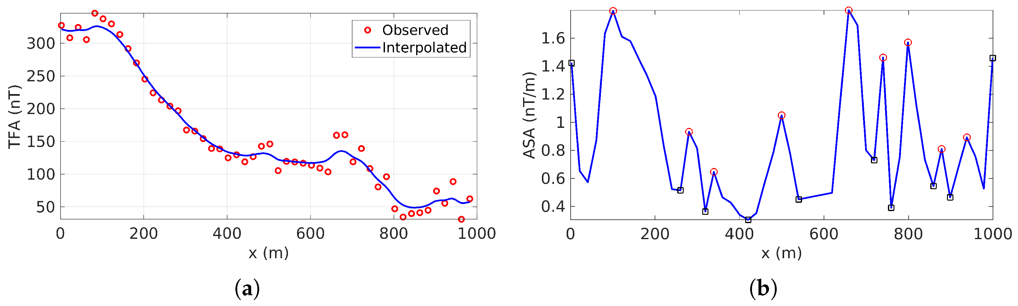
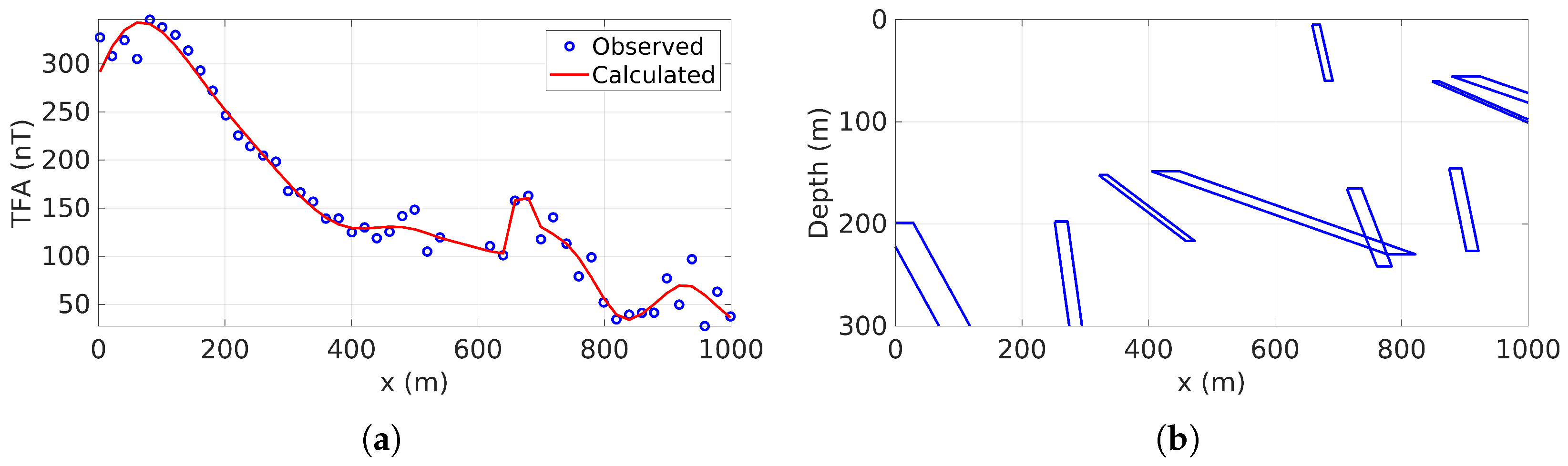
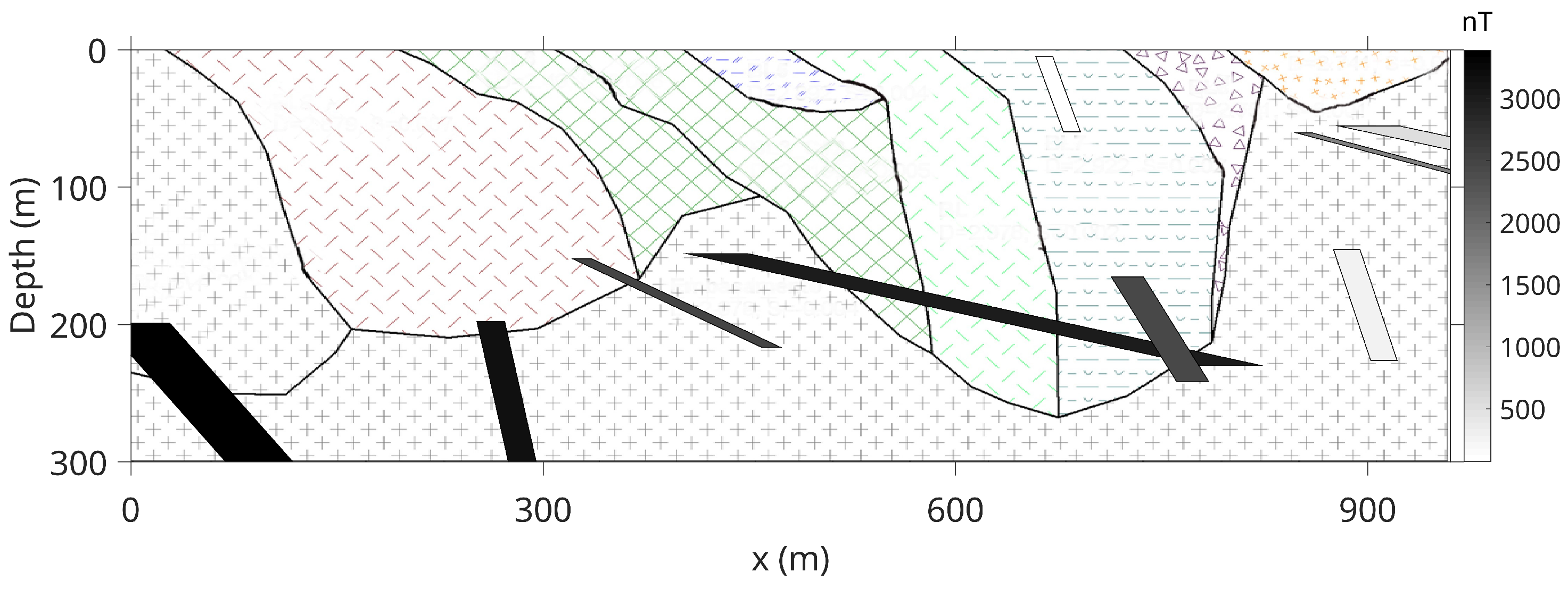
3.3. Laje Iron Ore Deposit

In this second field example, we employed a magnetic profile from a ground survey in Laje, Bahia, Brazil [29]. The geology of the profile under study (Figure 6) is primarily composed of Precambrian rocks, which to the east are overlain by the Mesozoic Camamu Basin, Tertiary Barreiras Formation sedimentary rocks, and Quaternary sediments. These Precambrian rocks, mainly metamorphosed into amphibolite and granulite, form two main tectonic units: the Jequié Block (JB) to the west and the Itabuna-Salvador-Curaçá Block (ISCB) to the east. The ISCB and JB, along with the Serrinha and Gavião blocks, collided during the Paleoproterozoic orogenic events, resulting in the formation of the São Francisco Craton in the state of Bahia, Brazil [45]. These collisional transition zones are important for metallic mineralizations of possible economic interest, as they are favorable sites for the absorption of mineralized solutions that can lead to the formation of ore deposits, including iron deposits and banded iron formations [46,47]. The study area also includes Mesozoic and Quaternary sediments. The profile under study is located in the JB unit but may contain remnants of the ISCB (Figure 6). The presence of intrusive bodies and mineralization in the region suggests significant mineral potential.

Figure 7a shows Line 3 from [29], between points 9A and 9B, a NW-SE profile with sampling interval of about 20 m, and its least-squares interpolation using finite elements with B-splines [48]. The RMS = 13.819 nT between the observed and interpolated profiles was used to estimate the reference misfit ${\mathrm{\Phi }}_{ref}$. Moreover, we estimated the sources’ centers from the locations of the local maxima of the Analytic Signal Amplitude (ASA) to estimate the horizontal locations of the tops of the causative bodies [49]. This criterion provided $n_d=9$ sources (red circles in Figure 7b). The search intervals for ${\overline{x}}_i$, $1\le i\le n_d$, are given by consecutive minima of ASA and the profile endpoints (black squares on Figure 7b).

The MH method and the hybrid MH-LM methods with $n_{LM}=1,2,4,8$ have quickly reached ${\mathrm{\Phi }}_{ref}$, as shown by the low number of chains in

Table 5. Number of chains, average chain length, and RMS errors of the MH ($n_{LM}=0$) and MH-LM ($n_{LM}=1,\dots ,8$) methods for the Laje iron ore deposit.

${\mathit{n}}_{\mathbf{LM}}$	${\mathit{n}}_{\mathit{c}}$	$\overline{\mathit{n}}$	RMS (nT)
0	21	154,716	13.415
1	12	109,833	12.250
2	10	158,796	13.772
4	13	250,195	13.223
8	1	429,516	13.664

.

Table 6. Search intervals and inverted parameters by the MH-LM method with $n_{LM}=8$ for the Laje iron ore deposit. The search intervals of the prism centers are given by consecutive minima of ASA and the profile endpoints (black squares on Figure 7b).

	$\mathit{\beta }{(}^{\circ })$	$\mathit{\theta }{(}^{\circ })$	h (m)	t (m)	K (nT)	$\overline{\mathit{x}}$ (m)	d (m)
Interval	−180 to 180	0 to 90	0 to 200	50 to 200	0 to 4000	see caption	5 to 25
Prism 1	−179.402	48.414	199.058	197.119	3387.864	3.761	24.430
Prism 2	−178.783	77.361	197.720	196.879	3164.380	261.752	10.103
Prism 3	−164.691	25.117	152.085	64.518	2488.640	328.117	6.874
Prism 4	−164.402	12.306	148.394	81.313	3023.467	426.551	22.283
Prism 5	−172.033	69.814	4.903	54.907	79.134	664.527	6.161
Prism 6	−175.235	58.055	165.336	76.151	2406.299	725.036	11.667
Prism 7	171.985	14.870	60.530	79.416	1695.706	854.040	5.685
Prism 8	−42.077	71.502	145.492	80.779	275.657	884.711	9.601
Prism 9	−173.293	12.044	55.391	56.675	504.832	900.702	22.145

shows the search intervals and the inverted parameters for $n_{LM}=8$. The dips of the sources were constrained to the east direction, whereas the top depths and half-widths were constrained to the values observed in the inverted model proposed by [29]. It is important to highlight that the effect of remanence is related to the parameter $\beta$ associated with the proposed algorithm, thus this effect is considered in the resulting magnetic model obtained. Furthermore, the interpretation adopted used as reference the model developed in [29] and involved determining the position of the causative body based on extracting the regional field and using the hybrid MH-LM method.

The fitness between the observed data and the magnetic anomaly estimated by the MH-LM method with $n_{LM}=8$ is shown in Figure 8a. In this figure, the system of finite prisms influencing the amplitude and shape of the interpreted magnetic anomaly is also observed. This inverse modeling allowed the definition of the geometry of nine prismatic magnetic sources in the basement rocks, with magnetic amplitudes ranging from 79.134 to 3387.864 nT, indicating bodies predominantly dipping to the east (see Figure 8b). Its main application is to determine the position of the top and base, either from dipping contacts between two media with distinct susceptibility values or fault zones in the basement. These prisms delineate the geometry of large contrasts between aggregated magnetic sources rather than the exact geometry of these sources. We acknowledge the limitation of this modeling due to the non-truly 2D nature of the bodies.

The mentioned profile, up to a distance of 700 m, shows magnetic magnitude values that may indicate bodies with high susceptibility, suggesting fractured zones of mafic lithology with metallic mineral input. The amplitude decreases for distances greater than 800 m, indicating a reduction in susceptibility, suggesting a progressive enrichment of felsic composition and depletion of magnetic minerals towards the east of the profile. For depths less than 100 m, there is a possibility of shallower magnetic contacts on the eastern edge of the profile. Below this depth, prismatic bodies are identified, with the deepest extending to depths above 300 m. The concentration of these prisms suggests an enrichment of magnetic minerals at depths greater than 100 m and to the east of the profile under study. It is expected that combining this interpretation with other geophysical methods can provide important indications of areas suitable for future exploration of iron ore bodies.The mentioned profile, for depths less than 100 m, reveals the possibility of shallower magnetic contacts on the eastern edge of the profile. Below this depth, prismatic bodies are identified, with the deepest extending to depths above 300 m.

Figure 9 shows a comparison between the results presented in Figure 8b and the geophysical model obtained in [29] based on magnetic and gravimetric data. Both interpretations assume that the prisms exhibit eastward dips. Additionally, the top of the prismatic bodies interpreted in this study is consistent with the deeper levels of the basement in the western part of the profile and with the uplifted basement in its eastern part, which corroborates the model developed by [29].

4. Conclusions

We have introduced an improved method based on the Metropolis-Hasting algorithm and the Levenberg-Marquardt method to invert magnetic profiles due to multiple dike-like sources with finite depths. This method provides information on the top depth, thickness, half-width, horizontal location of the top center, geological dip, and two effective parameters that depend on the magnetization intensity and magnetization directions.

We tested the proposed method using synthetic and real anomalies. The model parameters obtained for the synthetic anomaly were close to the true parameter values in the noise-free and noisy cases. The results of real data from the Pima copper mine showed that the obtained parameters of the dike were similar to those detected by the known information. In contrast, the Laje iron ore deposit results indicated that the proposed method could effectively detect parameters of multiple dike-like sources in real applications.

Our approach relies on a priori knowledge about the number of prisms. In situations such as highly interfering sources with high and low magnetization, the analytic signal amplitude may not be suitable to estimate the number of prisms and their locations.

References

1. Hood, P. The Königsberger ratio and the dipping-dyke equation. Geophys. Prospect. 1964, 12, 440–456. [Google Scholar] [CrossRef]
2. Barongo, J.O. Method for depth estimation on aeromagnetic vertical gradient anomalies. Geophysics 1985, 50, 963–968. [Google Scholar] [CrossRef]
3. Gobashy, M.; Abdelazeem, M.; Abdrabou, M. Minerals and ore deposits exploration using meta-heuristic based optimization on magnetic data. Contrib. Geophys. Geod. 2020, 50, 161–199. [Google Scholar] [CrossRef]
4. Balkaya, Ç.; Kaftan, I. Inverse modelling via differential search algorithm for interpreting magnetic anomalies caused by 2D dyke-shaped bodies. J. Earth Syst. Sci. 2021, 130, 135. [Google Scholar] [CrossRef]
5. Biswas, A.; Rao, K.; Mondal, T.S. Inverse modeling and uncertainty assessment of magnetic data from 2D thick dipping dyke and application for mineral exploration. J. Appl. Geophys. 2022, 207, 104848. [Google Scholar] [CrossRef]
6. Ai, H.; Ekinci, Y.L.; Balkaya, Ç.; Essa, K.S. Inversion of geomagnetic anomalies caused by ore masses using Hunger Games Search algorithm. Earth Space Sci. 2023, 10, e2023EA003002. [Google Scholar] [CrossRef]
7. Rao, B.S.R.; Murthy, I.V.R.; Rao, C.V. Two methods for computer interpretation of magnetic anomalies of dikes. Geophysics 1973, 38, 710–718. [Google Scholar] [CrossRef]
8. Won, I.J. Application of Gauss’s method to magnetic anomalies of dipping dikes. Geophysics 1981, 46, 211–215. [Google Scholar] [CrossRef]
9. Johnson, W.W. A least-squares method of interpreting magnetic anomalies caused by two-dimensional structures. Geophysics 1969, 34, 65–74. [Google Scholar] [CrossRef]
10. Ku, C.C.; Sharp, J.A. Werner deconvolution for automated magnetic interpretation and its refinement using Marquardt’s inverse modeling. Geophysics 1983, 48, 754–774. [Google Scholar] [CrossRef]
11. Marobhe, I.M. A versatile Turbo-Pascal program for optimization of magnetic anomalies caused by two-dimensional dike, prism, or slope models. Comput. Geosci. 1990, 16, 341–365. [Google Scholar] [CrossRef]
12. Biswas, A.; Parija, M.P.; Kumar, S. Global nonlinear optimization for the interpretation of source parameters from total gradient of gravity and magnetic anomalies caused by thin dyke. Ann. Geophys. 2017, 60, 0218. [Google Scholar] [CrossRef]
13. Kaftan, İ. Interpretation of magnetic anomalies using a genetic algorithm. Acta Geophys. 2017, 65, 627–634. [Google Scholar] [CrossRef]
14. Essa, K.S.; Elhussein, M. PSO (Particle Swarm Optimization) for interpretation of magnetic anomalies caused by simple geometrical structures. Pure Appl. Geophys. 2018, 175, 3539–3553. [Google Scholar] [CrossRef]
15. Ekwok, S.E.; Eldosouky, A.M.; Essa, K.S.; George, A.M.; Abdelrahman, K.; Fnais, M.S.; Andráš, P.; Akaerue, E.I.; Akpan, A.E. Particle swarm optimization (PSO) of high-quality magnetic data of the Obudu Basement Complex, Nigeria. Minerals 2023, 13, 1209. [Google Scholar] [CrossRef]
16. Ekinci, Y.L.; Balkaya, Ç.; Göktürkler, G.; Turan, S. Model parameter estimations from residual gravity anomalies due to simple-shaped sources using differential evolution algorithm. J. Appl. Geophys. 2016, 129, 133–147. [Google Scholar] [CrossRef]
17. Ai, H.; Ekinci, Y.L.; Balkaya, Ç.; Alvandi, A.; Ekinci, R.; Roy, A.; Su, K.; Pham, L.T. Modified Barnacles mating optimizing algorithm for the inversion of self-potential anomalies due to ore deposits. Nat. Resour. Res. 2024, 33, 1073–1102. [Google Scholar] [CrossRef]
18. Su, K.; Ai, H.; Alvandi, A.; Lyu, C.; Wei, X.; Qin, Z.; Tu, Y.; Yan, Y.; Nie, T. Hunger Games Search for the elucidation of gravity anomalies with application to geothermal energy investigations and volcanic activity studies. Open Geosci. 2024, 16, 20220641. [Google Scholar] [CrossRef]
19. Wigh, M.D.; Hansen, T.M.; Døssing, A. Inference of unexploded ordnance (UXO) by probabilistic inversion of magnetic data. Geophys. J. Int. 2020, 220, 37–58. [Google Scholar] [CrossRef]
20. Titus, W.J.; Titus, S.J.; Davis, J.R. A Bayesian approach to modeling 2D gravity data using polygons. Geophysics 2017, 82, G1–G21. [Google Scholar] [CrossRef]
21. Zunino, A.; Ghirotto, A.; Armadillo, E.; Fichtner, A. Hamiltonian Monte Carlo Probabilistic Joint Inversion of 2D (2.75 D) Gravity and Magnetic Data. Geophys. Res. Lett. 2022, 49, e2022GL099789. [Google Scholar] [CrossRef]
22. Mosegaard, K.; Sambridge, M. Monte Carlo analysis of inverse problems. Inverse Probl. 2002, 18, R29. [Google Scholar] [CrossRef]
23. Ben, U.C.; Akpan, A.E.; Mbonu, C.C.; Ebong, E.D. Novel methodology for interpretation of magnetic anomalies due to two-dimensional dipping dikes using the Manta Ray Foraging Optimization. J. Appl. Geophys. 2021, 192, 104405. [Google Scholar] [CrossRef]
24. Sen, M.K.; Stoffa, P.L. Global Optimization Methods in Geophysical Inversion, 2nd ed.; Cambridge University Press: Cambridge, UK, 2013. [Google Scholar]
25. Di Maio, R.; Milano, L.; Piegari, E. Modeling of magnetic anomalies generated by simple geological structures through Genetic-Price inversion algorithm. Phys. Earth Planet. Inter. 2020, 305, 106520. [Google Scholar] [CrossRef]
26. Talwani, M.; Heirtzler, J. Computation of magnetic anomalies caused by two-dimensional bodies of arbitrary shape. In Computers in the Mineral Industries; Part 1; Parks, G.A., Ed.; Stanford University Publications: Redwood City, CA, USA, 1964; pp. 464–480. [Google Scholar]
27. Al-Mamun, A.; Barber, J.; Ginting, V.; Pereira, F.; Rahunanthan, A. Contaminant transport forecasting in the subsurface using a Bayesian framework. Appl. Math. Comput. 2020, 387, 124980. [Google Scholar] [CrossRef]
28. Gay, S.P. Standard curves for interpretation of magnetic anomalies over long tabular bodies. Geophysics 1963, 28, 161–200. [Google Scholar] [CrossRef]
29. Sampaio, E.E.S.; Batista, J.C.; Santos, E.S.M. Interpretation of geophysical data for iron ore detailed survey in Laje, Bahia, Brazil. An. Acad. Bras. CiêNcias 2021, 93, e20200178. [Google Scholar] [CrossRef]
30. McGrath, P.H.; Hood, P.J. The dipping dike case: A computer curve-matching method of magnetic interpretation. Geophysics 1970, 35, 831–848. [Google Scholar] [CrossRef]
31. Mosegaard, K.; Tarantola, A. Monte Carlo sampling of solutions to inverse problems. J. Geophys. Res. Solid Earth 1995, 100, 12431–12447. [Google Scholar] [CrossRef]
32. Darroch, J.N. On the Distribution of the Number of Successes in Independent Trials. Ann. Math. Stat. 1964, 35, 1317–1321. [Google Scholar] [CrossRef]
33. Borges, M.R.; Pereira, F. A novel approach for subsurface characterization of coupled fluid flow and geomechanical deformation: The case of slightly compressible flows. Comput. Geosci. 2020, 24, 1693–1706. [Google Scholar] [CrossRef]
34. Gamerman, D.; Lopes, H.F. Markov Chain Monte Carlo: Stochastic Simulation for Bayesian Inference; Chapman & Hall/CRC Texts in Statistical Science; Taylor & Francis: Abingdon, UK, 2006. [Google Scholar] [CrossRef]
35. Yamashita, N.; Fukushima, M. On the rate of convergence of the Levenberg-Marquardt method. In Topics in Numerical Analysis: With Special Emphasis on Nonlinear Problems; Springer: Berlin/Heidelberg, Germany, 2001; pp. 239–249. [Google Scholar] [CrossRef]
36. Boos, E.; Gonçalves, D.S.; Bazán, F.S. Levenberg-Marquardt method with singular scaling and applications. Appl. Math. Comput. 2024, 474, 128688. [Google Scholar] [CrossRef]
37. Fernandes, J.A.; Azevedo, J.S.; Oliveira, S.P. A combined Markov Chain Monte Carlo and Levenberg-Marquardt inversion method for heterogeneous subsurface reservoir modeling. Discov. Appl. Sci. 2024, 6, 514. [Google Scholar] [CrossRef]
38. Raju, D.C.V. LIMAT: A computer program for least-squares inversion of magnetic anomalies over long tabular bodies. Comput. Geosci. 2003, 29, 91–98. [Google Scholar] [CrossRef]
39. Essa, K.S. A particle swarm optimization method for interpreting self-potential anomalies. J. Geophys. Eng. 2019, 16, 463–477. [Google Scholar] [CrossRef]
40. Pham, L.T.; Oksum, E.; Le, D.V.; Ferreira, F.J.F.; Le, S.T. Edge detection of potential field sources using the softsign function. Geocarto Int. 2022, 37, 4255–4268. [Google Scholar] [CrossRef]
41. Abdelrahman, E.M.; Sharafeldin, S.M. An iterative least-squares approach to depth determination from residual magnetic anomalies due to thin dikes. J. Appl. Geophys. 1996, 34, 213–220. [Google Scholar] [CrossRef]
42. Asfahani, J.; Tlas, M. A robust nonlinear inversion for the interpretation of magnetic anomalies caused by faults, thin dikes and spheres like structure using stochastic algorithms. Pure Appl. Geophys. 2007, 164, 2023–2042. [Google Scholar] [CrossRef]
43. Ekinci, Y.L. MATLAB-based algorithm to estimate depths of isolated thin dike-line sources using higher-order horizontal derivatives of magnetic anomalies. SpringerPlus 2016, 5, 1384. [Google Scholar] [CrossRef]
44. Dannemiller, N.; Li, Y. A new method for determination of magnetization direction. Geophysics 2006, 71, L69–L73. [Google Scholar] [CrossRef]
45. Barbosa, J.S.F.; Sabaté, P. Archean and Paleoproterozoic crust of the São Francisco craton, Bahia, Brazil: Geodynamic features. Precambrian Res. 2004, 133, 1–27. [Google Scholar] [CrossRef]
46. Smithies, R.H.; Bagas, L. High pressure amphibolite-granulite facies metamorphism in the Paleoproterozoic Rudall Complex, central Western Australia. Precambrian Res. 1997, 83, 243–265. [Google Scholar] [CrossRef]
47. Beukes, N.J.; Mukhopadhyay, J.; Gutzmer, J. Genesis of high-grade iron ores of the Archean Iron Ore Group around Noamundi, India. Econ. Geol. 2008, 103, 365–386. [Google Scholar] [CrossRef]
48. Inoue, H. A least-squares smooth fitting for irregularly spaced data: Finite-element approach using the cubic B-spline basis. Geophysics 1986, 51, 2051–2066. [Google Scholar] [CrossRef]
49. de Souza, J.; Oliveira, S.P.; Ferreira, F.J.F. Using parity decomposition for interpreting magnetic anomalies from dikes having arbitrary dip angles, induced and remanent magnetization. Geophysics 2020, 85, J51–J58. [Google Scholar] [CrossRef]
Figure 1. Simplified flowchart of the MH-LM algorithm.
Minerals 14 01054 g001
Figure 2. Magnetic profiles obtained by models with finite and infinite depth extent. (a) Synthetic model with finite sources (blue lines) and their extensions to infinity (red, dashed lines). (b) Magnetic anomalies.
Minerals 14 01054 g002
Figure 3. Observed synthetic data and magnetic anomaly calculated using the MH method (a) and the MH-LM method with n L M = 8 (b) in the noise-free case. (c,d) show the corresponding inverted models.
Minerals 14 01054 g003
Figure 4. Observed synthetic data and magnetic anomaly calculated using the MH method (a) and the MH-LM method with n L M = 8 (b) in the noisy case. (c,d) show the corresponding inverted models.
Minerals 14 01054 g004
Figure 5. (a) Observed data from the Pima copper mine and magnetic anomaly calculated using the MH-LM method with n L M = 8 . (b) Inverted model.
Minerals 14 01054 g005
Figure 6. Geological map and legend of the Valença sheet, modified from the map in [29], at a scale of 1:250,000. Points 9A and 9B mark the endpoints of the profile used in this research.
Minerals 14 01054 g006
Figure 7. (a) Observed data and its least-squares interpolation using finite elements with B-splines. (b) Analytic signal amplitude of the observed data.
Minerals 14 01054 g007
Figure 8. (a) Observed data from the Laje iron ore deposit and magnetic anomaly calculated using the MH-LM method with n L M = 8 . (b) Inverted model.
Minerals 14 01054 g008
Figure 9. Comparison between the result obtained in Figure 7b and the model from [29]. The colorbar refers to the amplitude parameters of the prisms.
Minerals 14 01054 g009