Monitoring of Mineral Processing Operations with Isolation Forests

Abstract

Reliable monitoring of mineral process systems is key to more efficient plant operation. Multivariate statistical process control based on principal component analysis is well-established in industry but may not be effective when dealing with dynamic nonlinear or transient processes, where process behavior may change rapidly from time to time. Although a large variety of nonlinear models have been proposed to address these problems, the monitoring of complex dynamic process systems remains challenging. Isolation forests are unsupervised machine learning models that provide an interesting approach to process monitoring that has not been explored extensively yet. In this investigation, this approach is compared with traditional multivariate statistical process monitoring based on principal component models. Three real-world case studies are considered. The first case study is based on coal flotation, the second is based on features extracted from a platinum group metal flotation froth; and the third is based on data from an industrial semi-autogenous grinding circuit. In each case, the models were trained on data representing normal operating conditions and then tested on new process data that were generally different from the training data to test their ability to identify these data as out-of-control. The isolation forest models performed better than the principal component models when the data were nonlinear, but not when the data associated with normal operation and faulty conditions were linearly separable, as was the case with the flotation data.

1. Introduction

Effective monitoring of process circuits is critical to efficient operation and key to predictive maintenance of equipment [1]. In particular, identification of process operations that may not obviously deviate from normal or optimal operating conditions can be difficult, especially when dealing with nonlinear systems. For example, grinding is influenced by a combination of factors, including mill design, operational parameters such as rotational speed, feed rate, and slurry density, and the characteristics of the mineral being processed. These factors interact in complex ways, leading to nonlinear responses that can be difficult to model and control. The same goes for froth flotation, where multiple variables have to be controlled simultaneously to optimize recovery and grade [2,3]. The interactions between these variables can create nonlinear behavior that complicates control strategies.

Process monitoring would typically be based on models capable of predicting the state of the process, whether it is in control or not, when presented with measurements of operational conditions. Although fundamental models can be used for this purpose, data-based models are more common, as these can be developed more rapidly and provide more reliable results than first-principle models. The disadvantage is that they may be more costly to maintain. Furthermore, monitoring of plant operations can either be supervised or unsupervised.

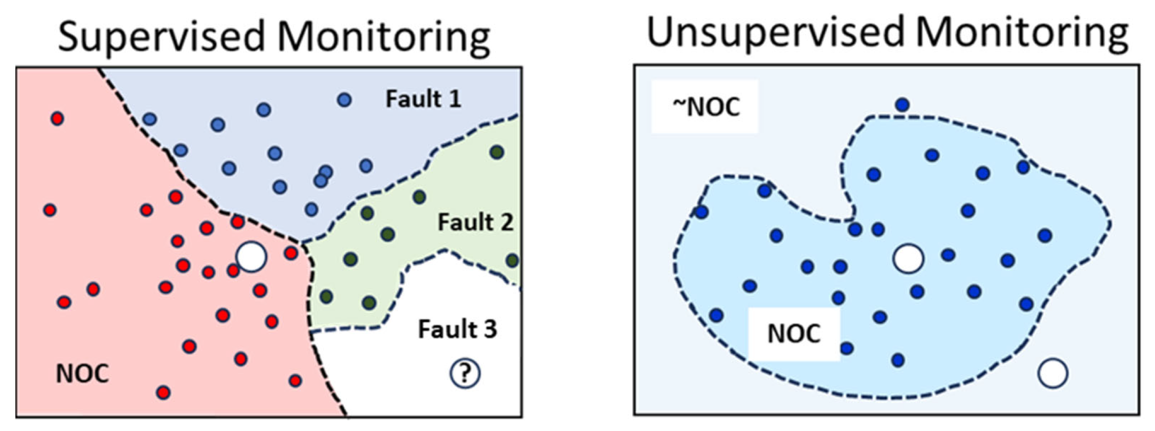
With supervised monitoring, the model is trained on labeled data from normal operating conditions (NOCs) as well as data from known fault conditions. Well-established models that are used for classification can be used for this purpose, such as random forests, boosted trees, or deep neural networks, as is the case in more recent studies [4,5,6]. The advantage of supervised monitoring is that known fault conditions can usually be rectified easily as their sources are well understood. The disadvantage of supervised process monitoring is that it may misclassify observations that do not belong to previously identified fault classes, as indicated schematically in the left-hand panel of Figure 1, where Fault 3 is an unknown fault that a machine learning model would be unable to identify or would misidentify, as it would not have been part of its training base. In addition, data from known fault conditions may be difficult to obtain.

In contrast, with unsupervised monitoring, the model is trained to simply predict whether the process is operating normally or in-control, or whether some unknown fault condition has arisen and the process is therefore out-of-control (e.g., [1,7,8,9]). This has the advantage that data regarding specific fault conditions, which may be scarce or unavailable, are not required to construct models. All that is required is data associated with normal operating conditions. The disadvantage of this approach is that it may be more challenging to rectify out-of-control operations as the source of the fault is generally unknown. In Figure 1, the right-hand panel indicates that a machine learning model constructs a representation (the dashed lines) of the NOC data. Any new data located on the outside of this decision surface would be classified as not NOC. The challenge is that these decision surfaces could have complex topologies in high-dimensional spaces that may not be easily learned from available process data.

In practice, multivariate approaches to unsupervised monitoring are mostly based on the use of latent variable methods, such as principal component analysis, that are capable of handling a wide variety of systems [10,11]. However, these methods may fail when process behavior is nonlinear.

Under these circumstances, nonlinear methods may be more suitable. Many such methods have been proposed in the past [12,13,14,15]. This includes, among other one-class classification methods [16], kernel principal component analysis [14,15,17,18], multiscale methods [19,20] and autoencoders [21,22]. These methods all address specific aspects of complex systems and may suffer from disadvantages related to robustness, training complexity that may become prohibitive when dealing with large-scale problems, computational cost, multimodal data, etc. As a consequence, the development of process monitoring systems remains an active area of research and development.

Isolation forests have the advantages of linear time complexity and a low memory requirement, which work well with high-volume data. Moreover, the algorithm relies upon the characteristics of anomalies, i.e., being few and different, in order to detect anomalies, which makes them suitable candidates for the development of unsupervised process monitoring systems. In this context, an anomaly is defined as a sample that can be isolated from the rest of the data with comparatively fewer partitions of the data space. This can be an effective approach to identifying samples in less dense regions of the data space, where traditional density-based methods might struggle when anomalies are globally rare. In addition, isolation forests are capable of capturing both linear and non-linear patterns. This flexibility makes them versatile for a wide range of anomaly detection tasks. Although they have been extensively applied in anomaly detection, their use in process monitoring frameworks has not been considered extensively as yet.

Therefore, in this investigation, the use of isolation forests that are trained on the NOC data set and then directly applied to new data that do not have the same statistical distribution as the training data are considered a novel framework for the monitoring of process systems.

2. Process Monitoring Methodology

From a process operator’s point of view, process data are available that have been recorded during normal process operation. The nature of these data would depend on the process or system under operation, but would typically consist of some set of variables or features that have been derived from equipment sensors. For example, this could include measurements of feed rates, feed densities, power consumption, in-line measurements of mineral grades, or features extracted from the vibrational spectra of equipment. Normally, these data would be collected under steady-state conditions. Typically, such data would have to be preprocessed to ensure a common time stamp (t), which may also require embedding with a time lag k and embedding dimension m in the form of X(t), X(t $-$ k), … X(t $-$ (m $-$ 1)k) prior to analysis. However, known direct indicators of process performance, such as recoveries or grades in flotation plants or the particle size of comminuted products in grinding circuits, would not be available.

2.1. Isolation Forests

Isolation forests (IFs) are ensembles of binary trees designed to recursively partition data [23], as indicated in Figure 2. A tree is grown by randomly splitting the feature space until each sample is contained in a terminal leaf node of the tree. Samples are assigned anomaly scores that are inversely related to the length of the branch between the root and the leaf node of the tree. In the final analysis, anomalies are identified based on their average scores across all the trees in the forest.

More formally, consider a data set $\mathbf{X}\in {\mathbb{R}}^{N\times M}$ consisting of $N$ samples and $M$ process variables ${\mathbf{x}}_j\in {\mathbb{R}}^M, j=\mathrm{1,2}, \dots M$, representative of normal operating conditions on the plant. The construction of a tree in the isolation forest is accomplished by generating nodes in the tree $\mathcal{t}\in T$ by randomly sampling a subset of the NOC training data of size $N_S\le N$. Subsequent to this, a variable $j\in M$, is randomly selected, together with a random split point $s$ in the interval $[{\mathbf{x}}_{j,min},{\mathbf{x}}_{j,max}]$. The subset of data ${\mathbf{x}}_j\le s$ is assigned to the left branch of the tree and ${\mathbf{x}}_j>s$, with the right branch in the tree $\mathcal{t}$.

The process is repeated for each of the descendent branches in the tree $\mathcal{t}$ and all the trees in the forest ($\mathcal{t}=1, 2, \dots T$), and terminated when the maximum tree depth ($L$) or the minimum terminal node size ($N_{min}$) is reached.

Once an isolation forest has been constructed, the expected path length, $h\left({\mathbf{x}}_i\right)$ required to isolate the sample ${\mathbf{x}}_i$ from the training data is computed from the mean of the path lengths in all the trees. The anomaly score $a\left({\mathbf{x}}_i\right)$, for the i’th sample in the training data is defined in Equation (1).

$$a\left({\mathbf{x}}_i\right)=2^{-E\left[h\left({\mathbf{x}}_i\right)\right]/c\left(n\right)}$$

(1)

In this equation, the expected path length is normalized by $c\left(n\right)$, which is the mean value of $h\left({\mathbf{x}}_i\right)$ for data sets of size $n$. This value can be computed using Equation (2), where $H\left(n\right)$ is the $n\prime th$ harmonic number, which can be approximated by $\ln \left(n\right)+\gamma$ = $\ln \left(n\right)+0.577$, where $\gamma$ is the Euler–Mascheroni constant [24].

$$c\left(n\right)=2H\left(n-1\right)-2(n-1)/n$$

(2)

This ensures that when $E\left[h\left({\mathbf{x}}_i\right)\right]=c\left(n\right)$, the anomaly score of the sample is $a\left({\mathbf{x}}_i\right)$ = 0.5. Moreover, for large values of $h\left({\mathbf{x}}_i\right)$, the anomaly score tends to 0, and for small values of $h\left({\mathbf{x}}_i\right)$ compared to $c\left(n\right)$, $a\left({\mathbf{x}}_i\right)$ tends to 1. This allows the specification of an anomaly threshold, $a_0 \in [0, 1]$ that would flag a sample ${\mathbf{x}}_i$ as an anomaly, that is, if $a\left({\mathbf{x}}_i\right)>a_0$.

Table 1. Hyperparameter settings of the isolation forests used in this investigation.

Parameter	Description	Value
T	Number of trees in the isolation forest	200
NS	Subsample size, no replacement	$\min (N,256$)
L	Maximum tree depth, ${L=\min (log}_2(N_s$)	$\le$8
MS	Feature sample size	$M$
C	Contamination factor	5%

summarizes the hyperparameters that were used to construct the isolation forests used in this investigation. These hyperparameters were mostly determined through trial and error, but a grid search can also be conducted to optimize the models more systematically. More specifically, the anomaly threshold was set to ensure the designation of 5% of the NOC data as anomalous, in keeping with a 95% control limit commonly used in statistical process control systems.

Even so, it should be noted that the performance of the isolation forest was not particularly sensitive to most of these parameters. For example, smaller forests with 50 trees showed somewhat lower performance than isolation forests with 100 or 200 trees, but not by a large margin. The only critical parameter was the anomaly threshold, which was set to ensure a Type II error (false negatives) of less than 5%. This threshold was not set directly but was determined by a contamination factor, which controls the expected proportion of anomalies in the data set. This factor was set at 5%, unless otherwise indicated.

Since first proposed by Liu et al. [25], isolation forests have become established in a variety of applications, including fraud detection, network intrusion detection, and outlier detection in data mining. To date, they have mostly been used in mineral exploration [26,27,28], but some applications have more recently appeared in diagnostic systems in mineral processing [29,30,31].

2.2. Application of Isolation Forest in Process Monitoring

Although isolation forests are machine learning algorithms designed for anomaly detection, they can be applied to a wide range of data analysis tasks, including process monitoring, although few such studies have been reported to date [31,32,33,34].

In the context of process monitoring, anomalies can represent deviations from normal or expected process behavior. By applying isolation forests to process data, unusual patterns, events, or behaviors can be identified that may indicate process deviations or abnormalities.

The IF model accomplishes this through the implicit construction of a decision surface, as illustrated in Figure 3. This figure shows observations of variables X and Y arranged in a square for illustrative purposes. The samples on the corners of the square indicated in red are more easily separated from the other samples, as they would require two splits of the data space only, while the other samples would require three or more splits.

If the samples on the corners of the square are considered to be anomalies, then the decision surface can be indicated by the red and blue-shaded areas on the graph. Data in the red-shaded regions would be considered out-of-control (OOC), and data in the blue-shaded areas would be in-control (IC), even if they are very far away from the NOC data, which is essentially comprised of the five points within the sample that were not considered to be anomalies.

2.3. Multivariate Statistical Process Control Based on Principal Component Analysis

The principal component model is constructed by expressing the data matrix with $N$ observations of $M$ variables $\mathbf{X}\in {\mathbb{R}}^{N\times M}$, as the product of a score matrix (${\mathbf{T}}_k\in {\mathbb{R}}^{N\times r}$) and a loading matrix (${\mathbf{P}}_k\in {\mathbb{R}}^{M\times r}$) consisting of a small number of principal components ($r<M$), as well as a residual matrix (${\mathbf{E}}_r$) [35].

$$\mathbf{X}={\mathbf{T}}_r{\mathbf{P}}_r^{\prime }+{\mathbf{E}}_r$$

(3)

For the $i$’th observation, the process control diagnostics are the Hotelling’s $T_i^2$ statistic and the squared prediction error, or $Q_i$-statistic, as indicated in Equations (4) and (5), respectively. These statistics can be explained by considering that the principal component model is based on a plane that is fitted through the data if there are two variables, or more generally, a hyperplane when there are more than two variables. Hotelling’s $T_i^2$ statistic is based on the projections of the data onto the principal component plane and captures the distance of each such projected point from the center of the plane.

Likewise, the $Q$-statistic accounts for the distance of the point from the plane. These two statistics are complementary in that points may be close to the plant but far from the center, or they may be projected close to the center of the plane but from a distance far away from the plane. In both of these cases, only one of the statistics will be able to identify the point as OOC. In Equations (4) and (5), ${\mathbf{x}}_i$, ${\mathbf{t}}_i$ and ${\mathbf{e}}_i$ are the i’th sample, principal component score, and residual.

$$T_i^2={\mathit{t}}_i{\mathit{\lambda }}_r^{-1}{\mathit{t}}_i^{\prime }={\mathit{x}}_i{\mathbf{P}}_r{\mathit{\lambda }}_r^{-1}{\mathbf{P}}_r^{\prime }{\mathit{x}}_i^{\prime }$$

(4)

$$Q_i={\mathit{e}}_i{\mathit{e}}_i^{\prime }={\mathit{x}}_i({\mathbf{I}}_r-{\mathbf{P}}_r{\mathbf{P}}_r^{\prime }){\mathit{x}}_i^{\prime }$$

(5)

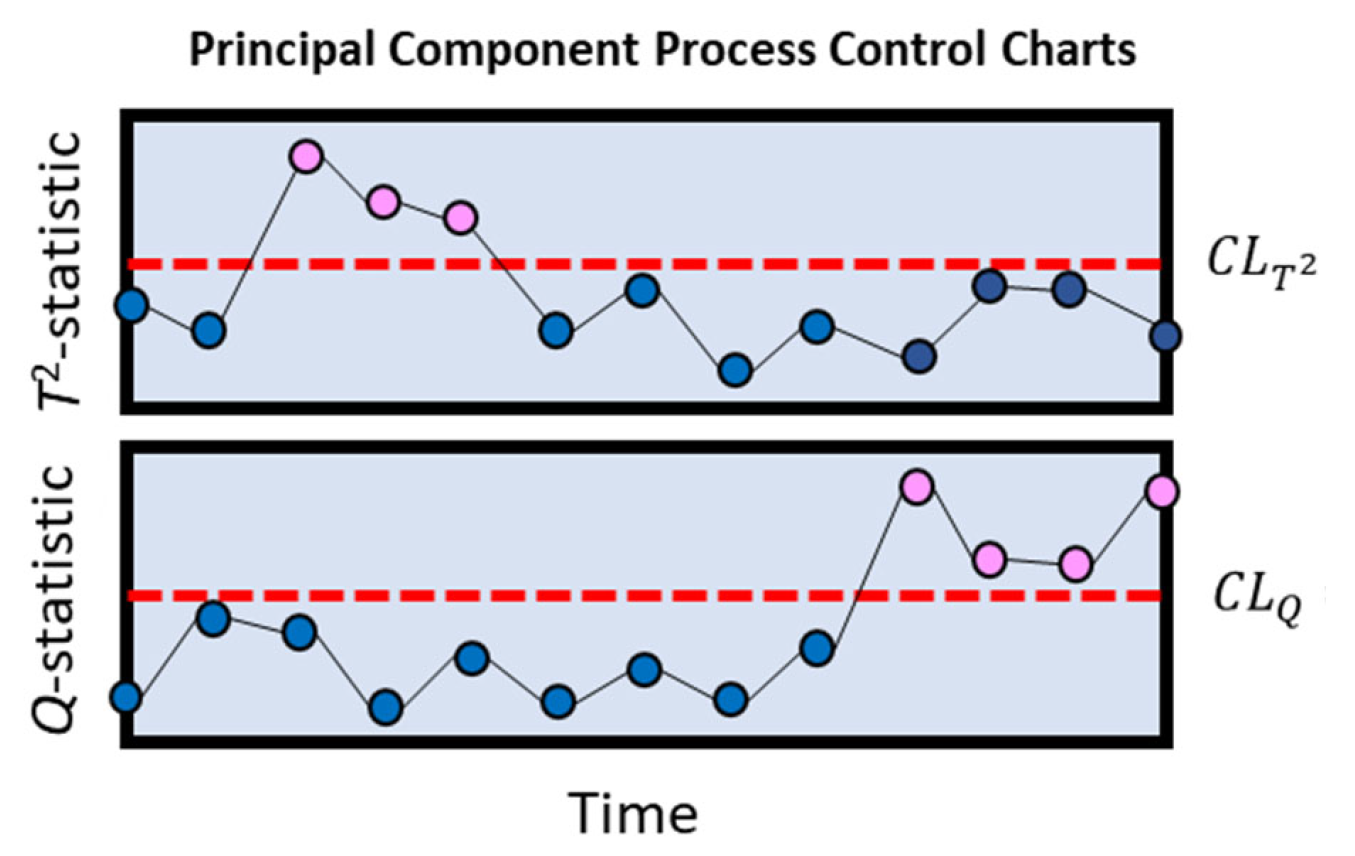
Monitoring of the process is based on a control chart for each of the two statistics ($T_i^2$ and $Q_i$), each provided with an appropriate control limit, as indicated by Equations (6)–(9).

$${CL}_{T^2}=\frac{r(N+1)(N-1)}{N^2-Nr}{F}_{(\alpha ,r,N-r)}$$

(6)

$${CL}_Q={\theta }_1{\left(\frac{z_{\alpha }\sqrt{2{\theta }_2{h}_0^2}}{{\theta }_1}+\frac{{\theta }_2{h}_0(h_0-1)}{{\theta }_1^2}+1\right)}^{1/h_0}$$

(7)

$$h_0=1-\frac{2{\theta }_1{\theta }_3}{3{\theta }_2^2}$$

(8)

$${\theta }_j=\sum _{i=r+1}^M{\lambda }_i^j$$

(9)

Equation (6), $F_{(\alpha ,r,N-r)}$ is the upper $\alpha$’th quantile of the F-distribution with r and N $-$ r degrees of freedom.

In Equations (7)–(9), $z_{\alpha }$ is the upper $\alpha$’th quantile of the standard normal distribution and ${\lambda }_i$ is the I’th eigenvalue of the principal component model. The process is considered to be out-of-control (OOC), if either $T_i^2>{CL}_{T^2}$ or $Q_i>{CL}_Q$, as illustrated in Figure 4.

When the data are not approximately normally distributed or the data distribution is unknown, the control limits can also be fitted to the training (NOC) data of the model, as was conducted in this investigation.

The following case studies illustrate and assess the performance of the IF and PCA-based methods on a comparative basis.

3. Case Study 1: Coal Flotation

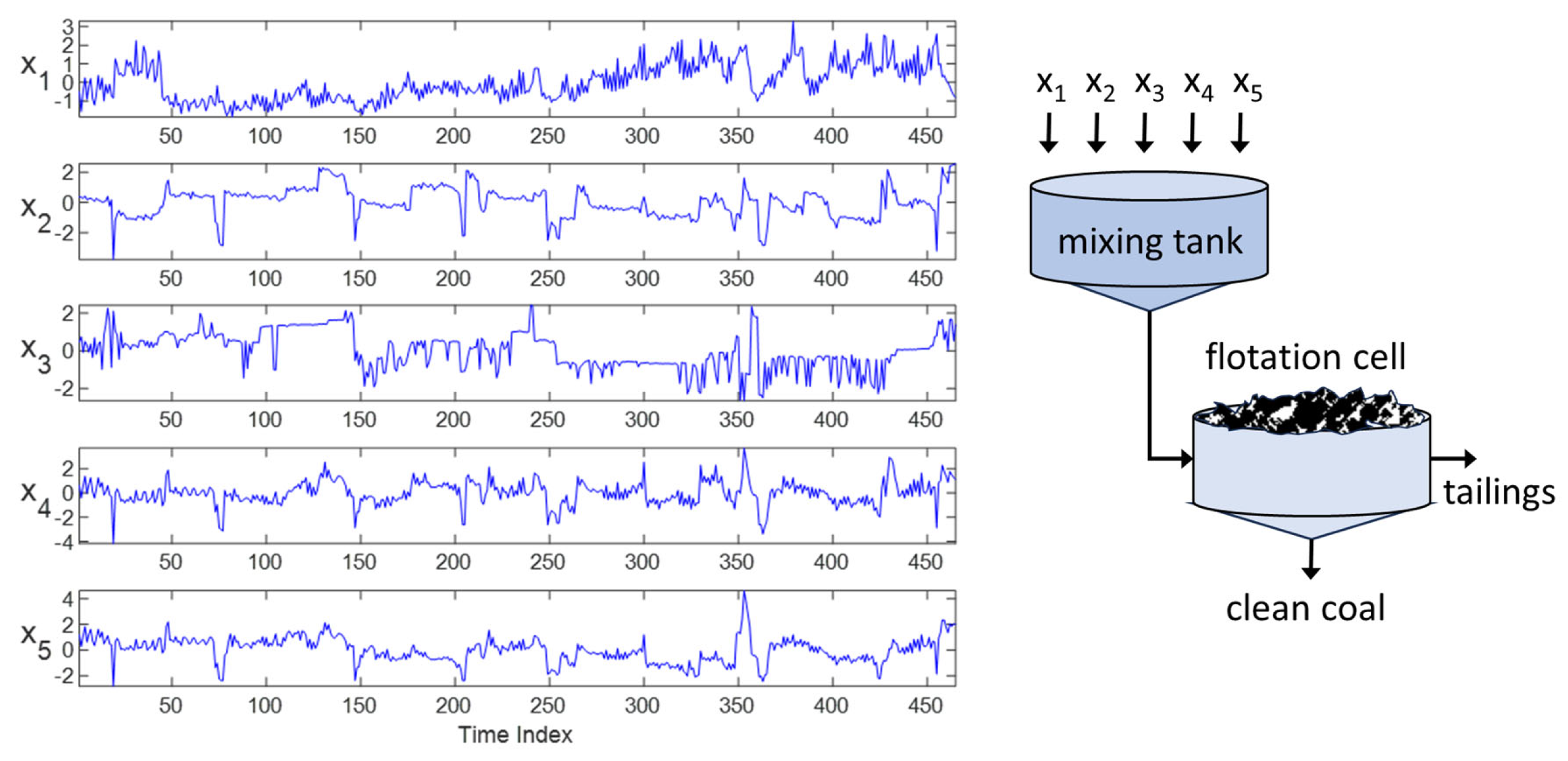
In the first case study, the flotation of coal to separate fine coal from a coal slurry mixture is considered. Five variables were measured, namely the flow rate of the raw slurry into the mixing tank (x₁), the density of the slurry (x₂), the flow rate of water into the mixing tank (x₃), the flow rate of frother into the tank (x₄), as well as the flow rate of the kerosene collector into the tank (x₅), as shown in Figure 5.

A training data set ($X_{NOC}$) consisting of 200 NOC samples constituted normal operating conditions, while a test data set containing 65 samples with the same distribution as the training data and 200 samples different from the NOC data constituted the NEW data ($X_{NEW}$).

Multiple runs were made to fit the models, each time with a different training and test data set. At each run, an isolation forest with 200 trees and a contamination factor of C = 0.05 was fitted to the training data consisting of 200 samples and tested on the test data set that consisted of 265 samples, 65 of which were NOC data and 200 of which were not.

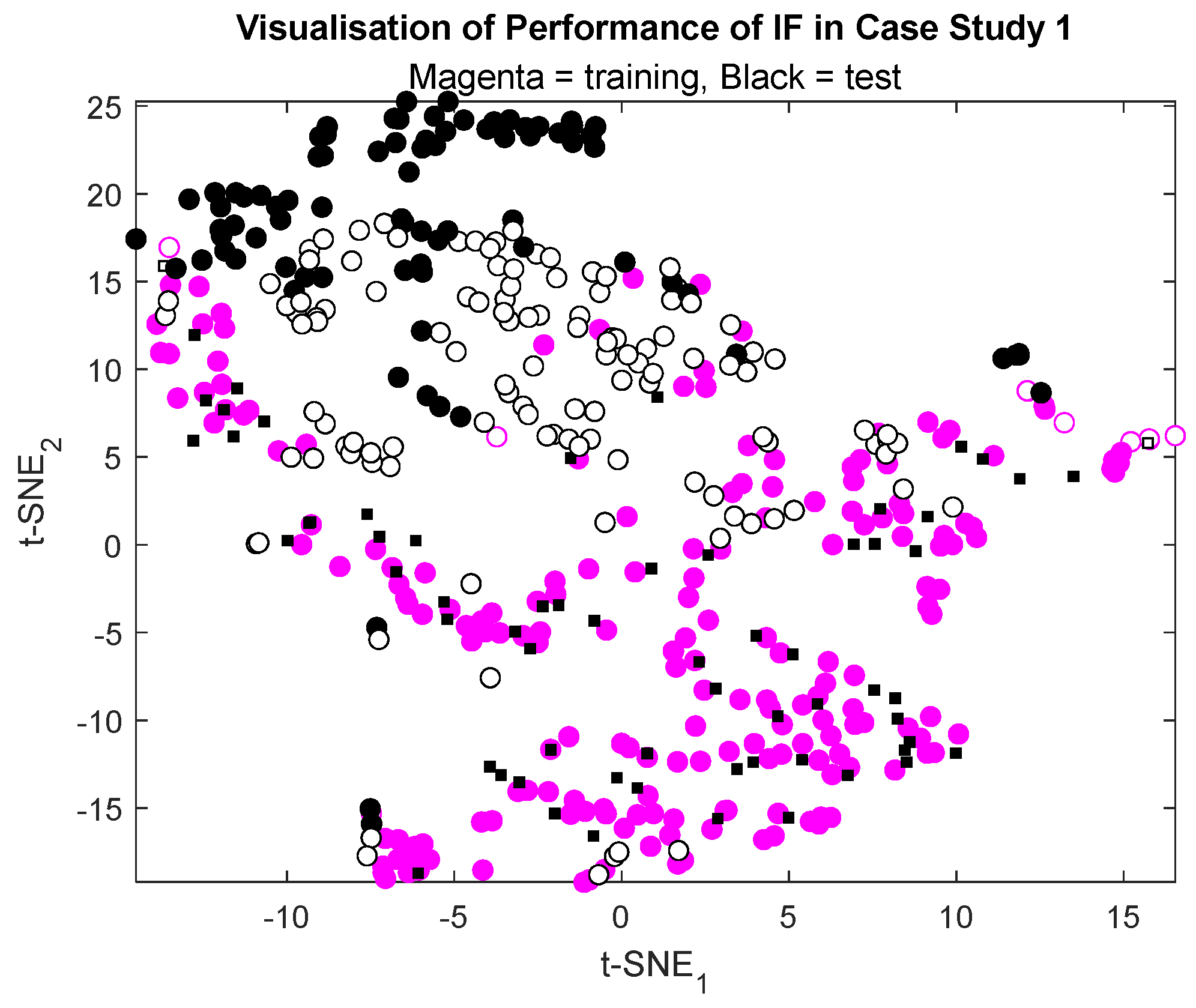
The typical performance of the IF on the data set can be visualized in Figure 6. In this figure, training (NOC) data are represented by magenta-colored markers and test data by black markers. Samples correctly identified as IC or OOC are indicated by solid markers. In the training data set, 5% of the samples are shown as empty markers, as determined by the contamination factor setting of 5%. The test data indicated by black markers are further characterized by circular and square markers. The square markers are test data, which are IC, while the circular markers are OOC. Solid black square markers therefore indicate that the model correctly identified these markers as IC in the test data set. In contrast, empty black circular markers indicate samples that were incorrectly identified by the IF model as IC.

In this particular case, the model correctly identified 96.9% of the 65 samples in the test set that were IC as such and 41% of the 200 samples in the test set that were OOC as such. The high hit rate of the model on the IC data in the test set is not unexpected, as these data had the same distribution as the data on which the IF model had been trained. In Figure 6, it can be seen that these data (black squares) are located within the same area on the chart as the training data of the model (magenta markers).

In

Table 2. Performance of IF and PC models with the coal flotation data in Case Study 1.

Model/ Statistic	IF (C = 0.05, T = 1000)		PCA (2 Components)
	FP-Test	TP-Test	FP-Test	TP-Test
Average	6.0	32.0	1.9	28.0
Median	6.2	31.8	1.5	30.3
StDev	0.47	1.40	1.8	10.2
Minimum	4.6	30.0	0.0	2.00
Maximum	6.2	35.0	7.7	45.0
No of Runs	20	20	20	20

, the false positive rates of the optimal models on the test data (FP-test) are shown, together with the true positive rates on the test data (TP-test). The principal component model was based on two components and could on average correctly identify 28.0% of the out-of-control samples, although it had a marginally lower false positive rate on the test data than the IF model that could on average identify 32.0% of the OOC samples.

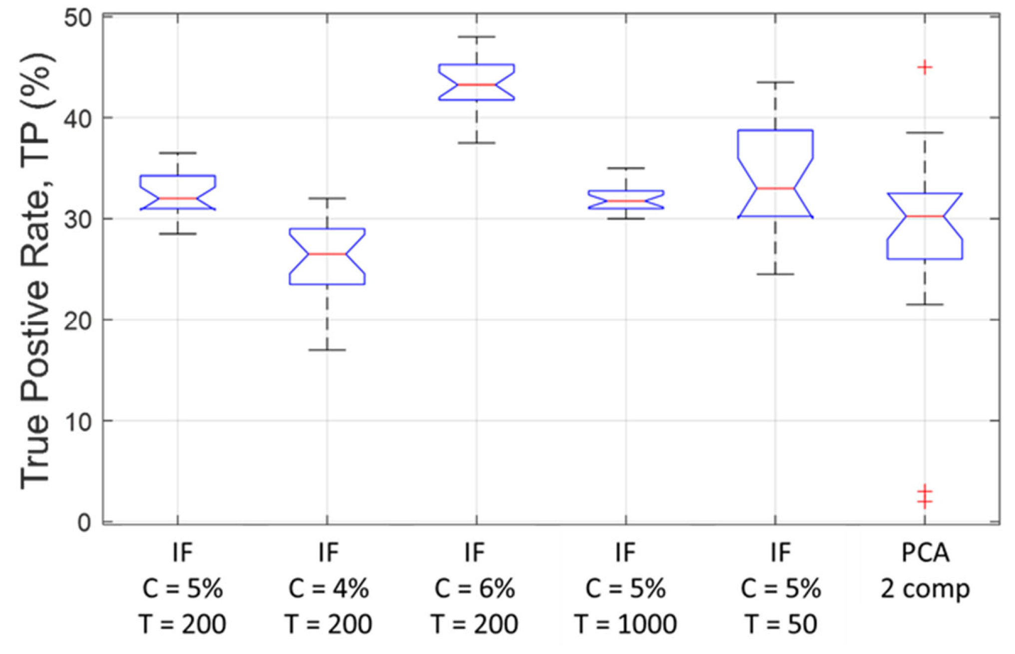
Figure 7 shows the effect of the contamination factor and isolation forest size on their performance in terms of their ability to correctly identify OOC samples in the test data. The performance of the principal component model is also included in this figure. In the boxplots shown in Figure 7, the central mark on each box indicates the median, and the bottom and top edges of the box indicate the 25th and 75th percentiles, respectively. The whiskers extend to the most extreme data points not considered outliers, and the outliers are plotted individually using the ‘+’ marker symbol.

In this figure, the first five boxes show the TP rates on the test data with IF models with various contamination factors (C) and trees (T). An increase in the contamination factor leads to an increase in the performance of the isolation forests, but at the expense of higher FP rates.

The box on the far right shows the performance of a principal component model with two components, which could explain 78% of the variance of the training data. Although the median TP rate of this model appears to be lower than that of the isolation forests with contamination factors of C = 5%, the overlapping notches suggest that these models may have performed statistically similarly. In addition, it is clear that the IF model with 1000 trees performed more consistently than the IF models with fewer trees (50 and 200), as well as the principal component model.

4. Case Study 2: Platinum Metal Group Flotation Froths

In the second case study, operational data from an industrial flotation plant are considered. A wealth of process information can be inferred from the appearance of the froth phase of flotation systems, which are routinely monitored in many industrial plants.

4.1. Operational Data

The small data set consisted of 297 samples of five gray-level co-occurrence matrix features that were extracted from images of platinum-group metal froths from a South African concentrator circuit. These studies were conducted in the early 1990s, and in this particular case, the original images and metadata associated with the images have not been retained. Nonetheless, the data serve as a practical real-world case study, given that the features were derived from froth structures that were classified by an experienced plant operator at the time.

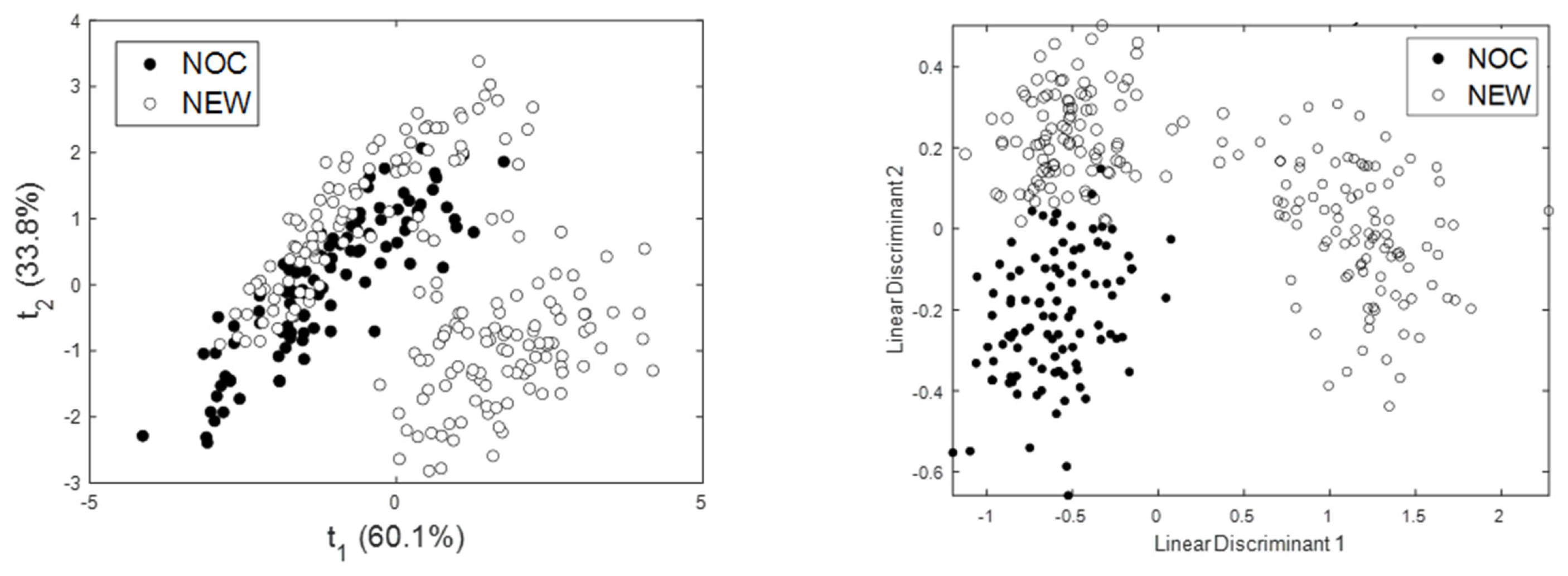
Projections of the samples with a principal component and linear discriminant model are shown in Figure 8. The first two principal components could explain approximately 93.9% of the variance of the data. The froth conditions associated with normal operating conditions (NOCs) are shown as black circles, while the out-of-control conditions are shown as white circles. The linear discriminant projection was manipulated to project the data into three groups, namely the NOC data and the NEW data, which consisted of two natural clusters. As indicated by the linear discriminant score plot, which by design projects the data onto a plane to maximize the separability of the groups, the data are linearly separable to a high degree.

The data that were presented to the models consisted of a training data set consisting of a random selection of 89 samples of the NOC data shown in Figure 8. The test data consisted of a random selection of 10 samples from the NOC data (not present in the training data set), as well as all of the data indicated as NEW in Figure 8. This gave a total of 208 samples in the test data set. Multiple runs were used to construct models based on different training and test data sets in each run, given the random selection of NOC data.

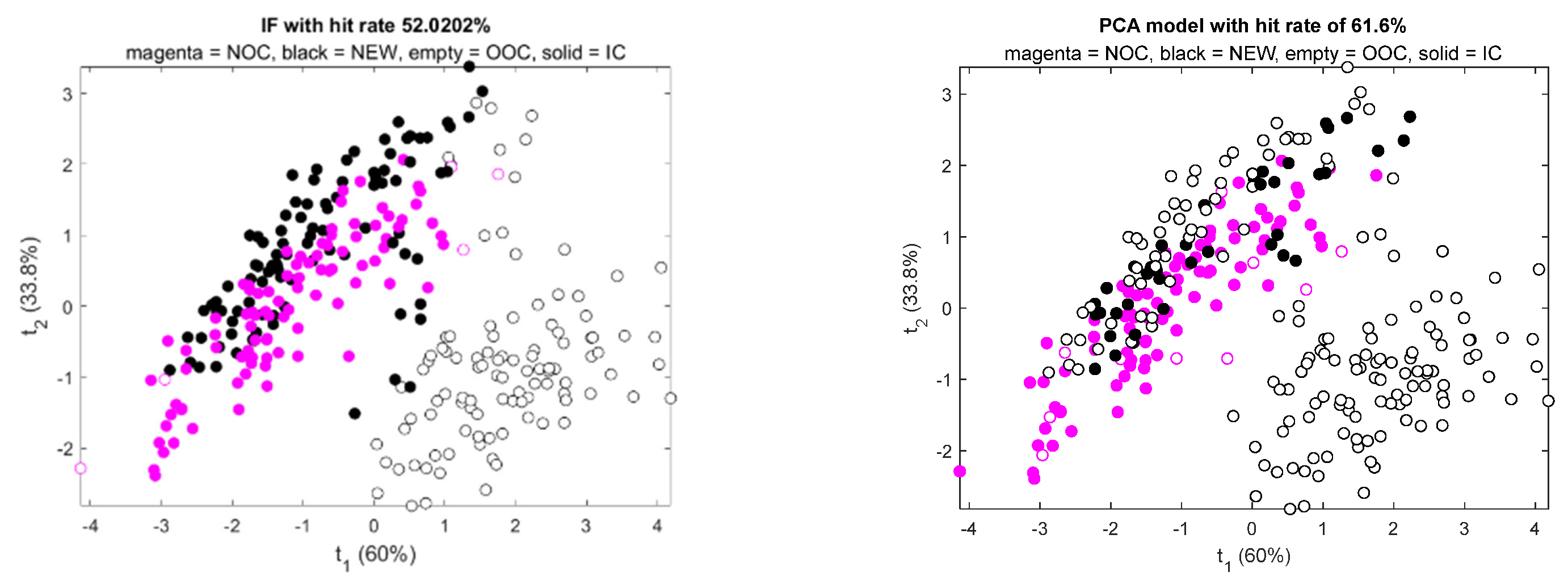
Figure 9 shows typical results from each of the two models. In each figure, the markers with magenta outlines indicate training data, while markers with black outlines indicate test data. Empty magenta markers indicate data that were assigned as OOC data by the models during training. Likewise, empty black markers indicate data that were assigned as OOC data by the models during testing. As can be seen from these graphs, both models could identify almost all of the NEW data in the cluster, separate from the NOC data, as out-of-control. The statistical performance of the models is discussed in more detail in the following sections.

4.2. Isolation Forest

As before,

Table 3. Performance of IF and PC models with the PGM data in Case Study 2.

Model/ Statistic	Isolation Forest (C = 0.05)			PC Model (2 Components)
	FP-Train	FP-Test	TP-Test	FP-Train	FP-Test	TP-Test
Average	4.5	6.0	53.0	5	2.0	65.0
Median	4.5	0	53.5	5	0	64.4
StDev	0	8.4	2.6	0	4.7	1.43
Minimum	4.5	0	49.0	5	0	63.9
Maximum	4.5	20	57.1	5	10	67.3
No of Runs	10	10	10	5	10	10

provides a summary of the performance of the two models. In this case, the PC model achieved a TP rate of 65.0% on average on the test data, with a FP rate of 2%, as compared with the 53.0% and 6.0% rates of the IF model.

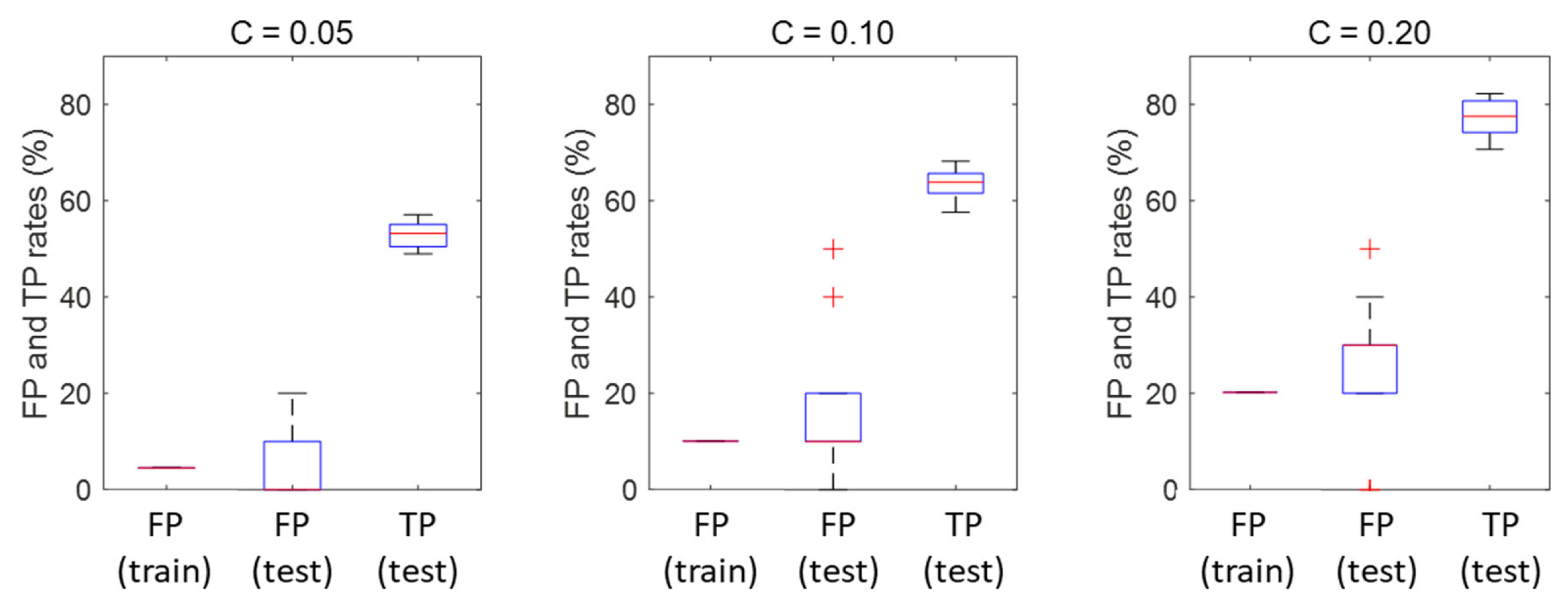
Figure 10 shows the performance of the IF model with different contamination factor values. As these C values increase, the true positive rates of the IF models also improve. With a C-value of 0.05, it shows a true positive rate on the test set with a median value of 53.5%. This increases to more than 60% and more than 70% at C-values of 0.10 and 0.20, but also with a concomitant increase in the false positive rates on the test data, which increases from approximately 5% to 10% and close to 30% at respective contamination factors of 5%, 10%, and 20%.

4.3. Multivariate Statistical Process Monitoring Based on Principal Component Analysis

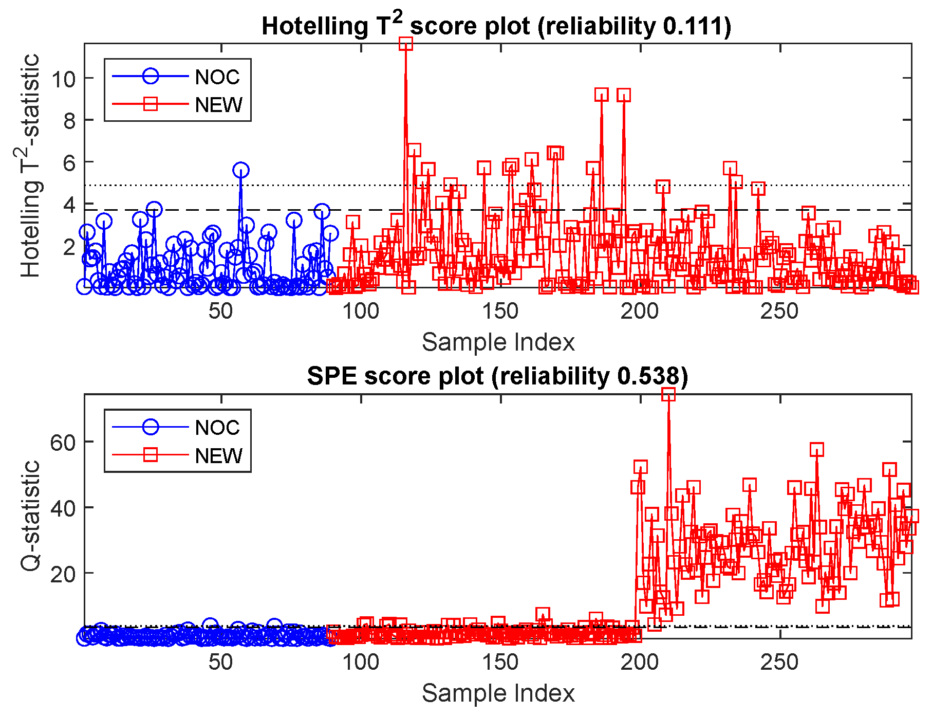
The Hotelling’s T² and Q score plots of the principal component model are shown in Figure 11, where the NOC data are indicated by blue circles and the NEW data by red squares. The 95% and 99% control limits on the graphs are indicated by the coarse and finely dashed horizontal lines on the graphs. Data exceeding the 95% control limits were considered to be out-of-control. This includes approximately 5% of the NOC data (blue markers with indices from 1 to 89).

As can be seen from Figure 11, the cluster of new data separate from the NOC data in Figure 9 (samples 199 to 297) are easily detected by the Q-statistic of the model since these data are far from the principal component plane fitted to the NOC data.

Hotelling’s T² and SPE statistics could collectively explain 68.7% of the new data as out-of-control, with a false positive rate of <5%. This is significantly better than what could be obtained with the isolation forest, which had similar false-positive rates of less than 5% on the test data.

5. Case Study 3: Monitoring of a SAG Circuit

5.1. Operational Data

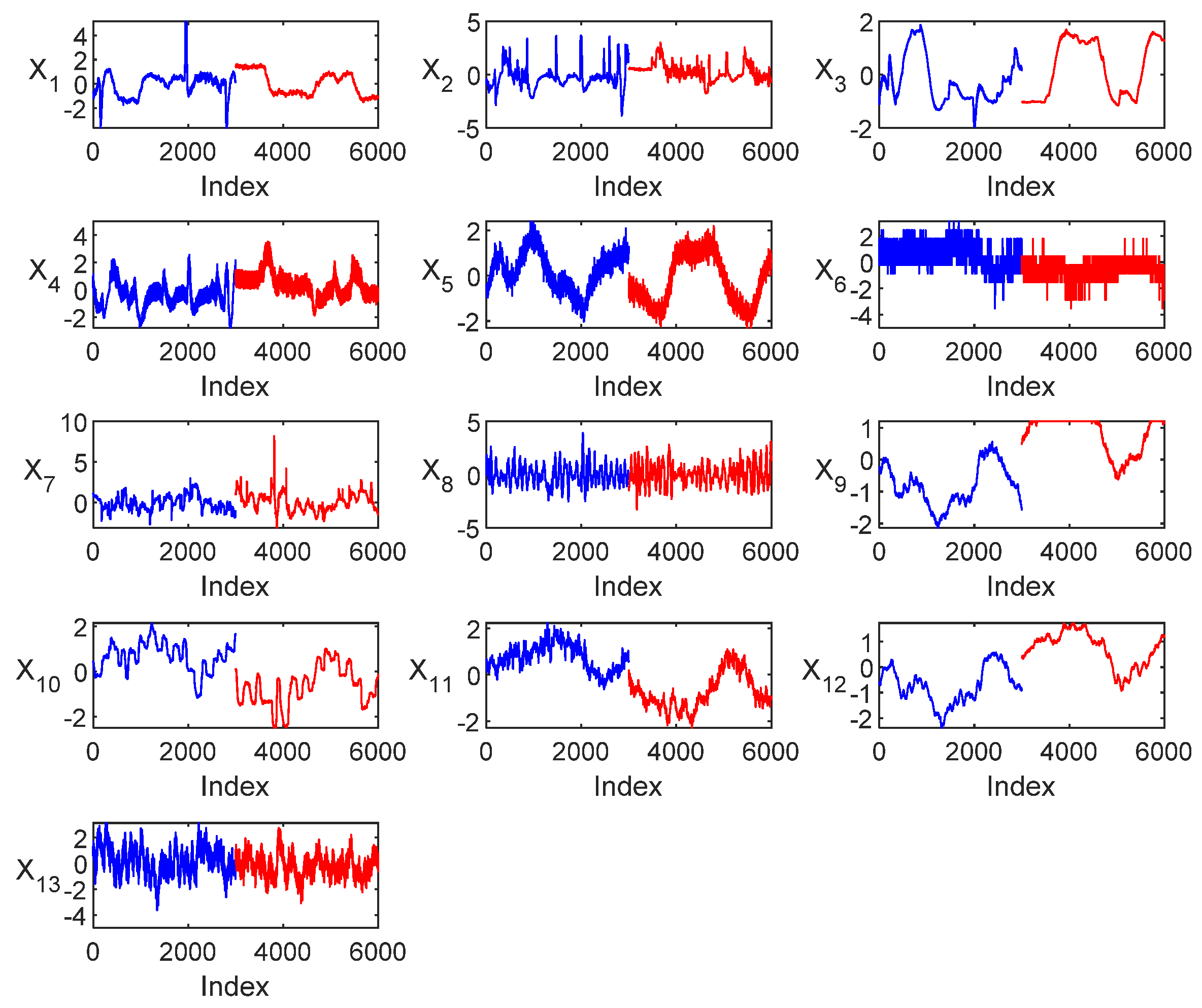
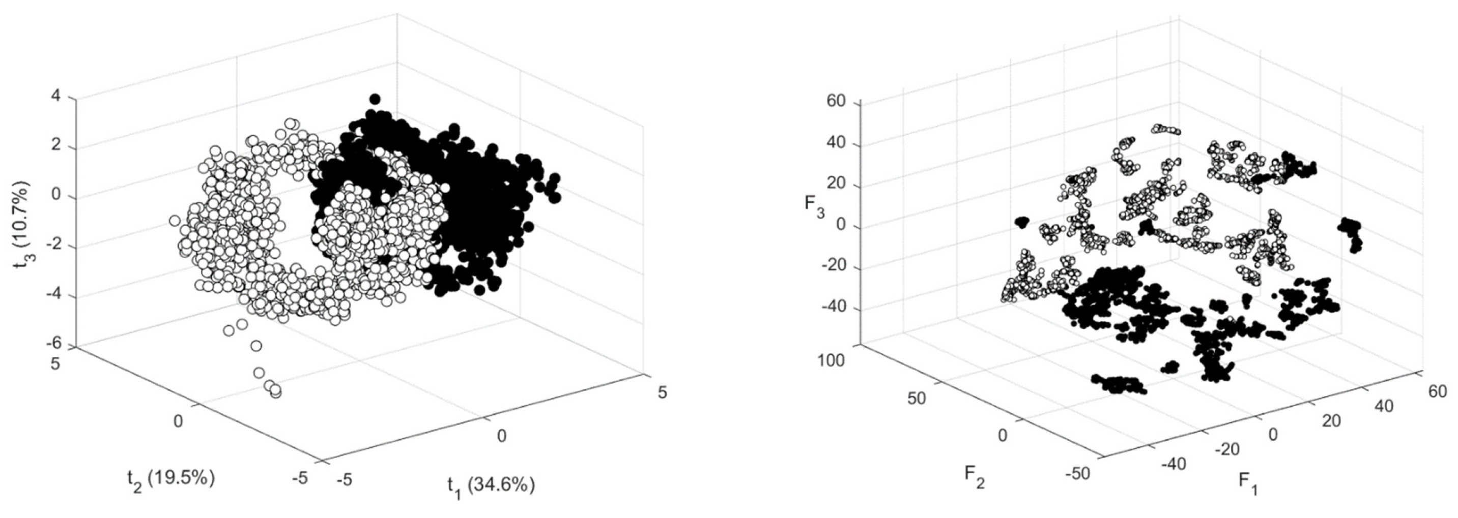
The scaled operational data, shown in Figure 12, consisted of 6000 samples spanning 13 operational variables that characterized the steady-state operation of an industrial semi-autogenous grinding circuit, as discussed by Groenewald et al. [36]. In this case study, the NOC data (indices 1–3000 in Figure 12) and NEW data (indices 3001–6000 in Figure 12) were collected over different periods of circuit operation. Visualization of the data with a t-SNE and principal component score plot, as shown in Figure 13, shows that the data have different highly separable distributions. The principal component score plot could account for 64.8% of the variance of the data. The t-SNE plot was constructed with a perplexity parameter of 50.

As a further assessment of the separability of the designated NOC and NEW data sets, a classification tree was constructed on a training data set consisting of 2500 samples randomly selected from both classes. The tree was able to discriminate with 99.4% accuracy between the NOC and NEW data in an independent test set consisting of the remainder of the NOC and NEW data.

As an aside, it should be noted that in practice, data would likely be selected over a continuous period where the process is in-control. It is also assumed that the data would be suitably prepared for the construction of models by dealing with missing data, outliers, and other issues related to data quality separately. In addition, once the models used for process monitoring have been constructed, they would typically be used to monitor individual samples collected in real-time. Recalibration of the model would be required when operational conditions change as a result of changes in the ore feed composition or other operational procedures.

The data on which the models were trained consisted of 2900 observations sampled randomly from the NOC data set. The test data set consisted of all the samples in the NEW data as well as 100 randomly selected samples from the NOC data, i.e., the data in the NOC data not included in the training data set. As before, these data could be used to assess the generation of false positives by the models.

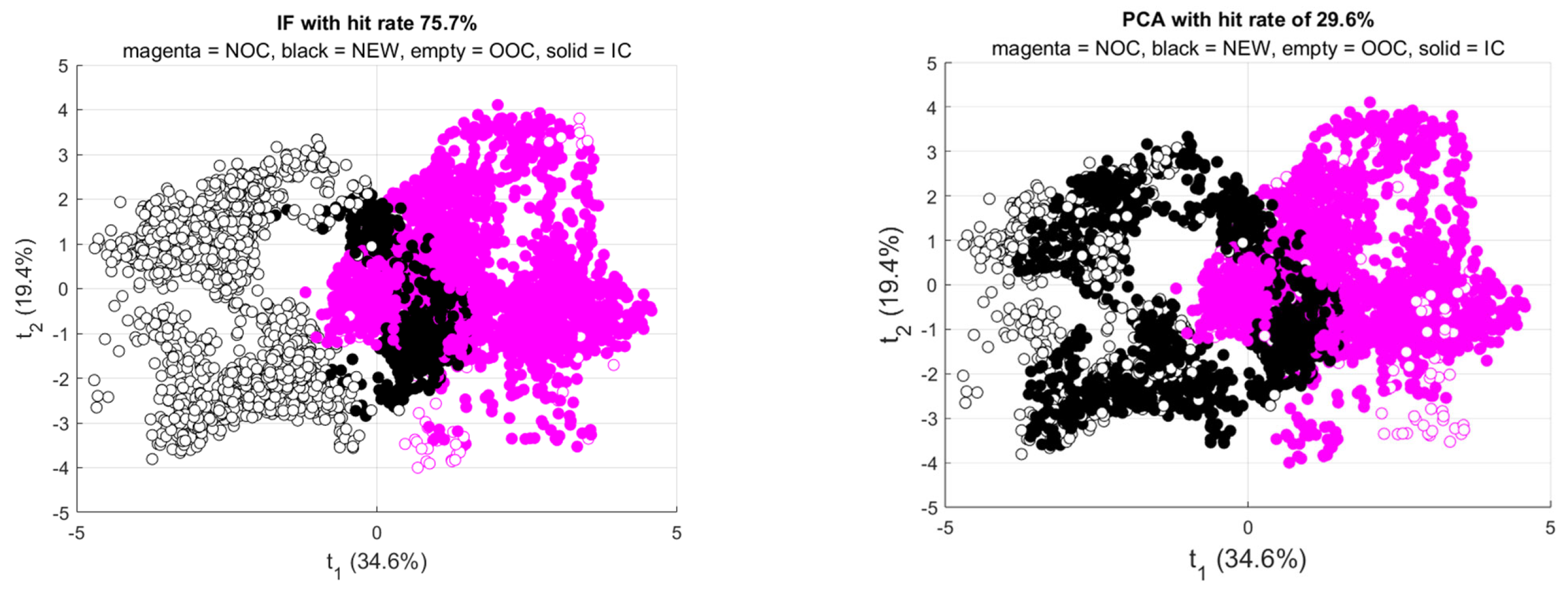
As before, models were run multiple times, which included the construction of new training and test sets for each run. Examples of the performance of the IF and PC models are shown in Figure 14 and discussed in more detail below.

5.2. Isolation Forest

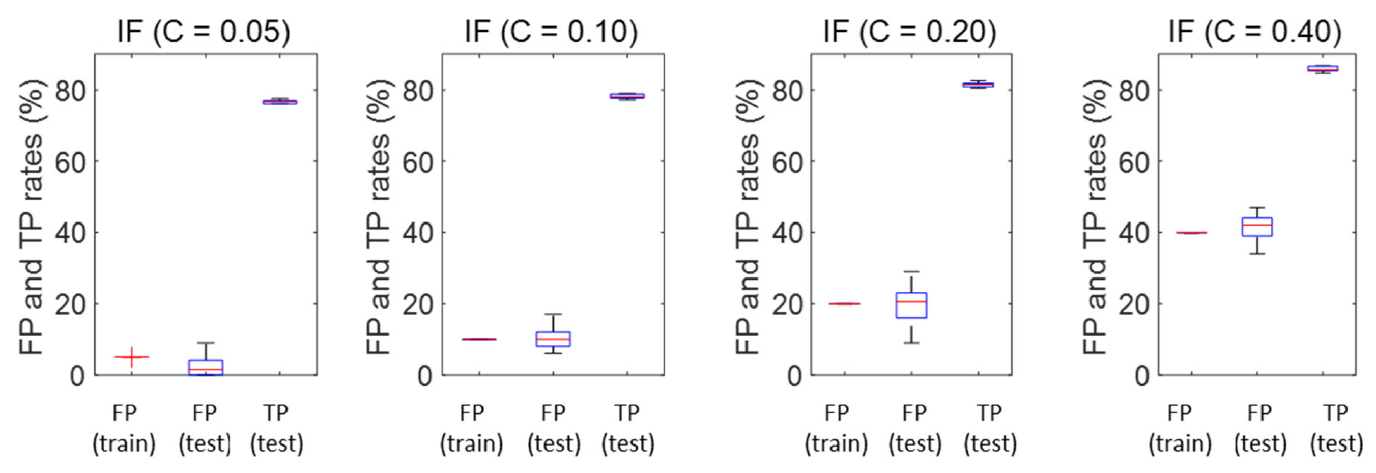
Figure 15 shows the performance of the IF model based on ten runs. The box plot on the left in the figure shows the false positive rate generated by the model on the NOC data, which was 5% by design. The box in the middle shows the false positive rate on the test data, which averaged 4.4%. The box on the right shows the true positive rate, which averaged 76.3%, as indicated in

Table 4. Performance of the IF and PC models with the SAG circuit data in Case Study 3.

Model/ Statistic	Isolation Forest (C = 0.05)			PC Model (5 Components)
	FP-Train	FP-Test	TP-Test	FP-Train	FP-Test	TP-Test
Average	5.0	4.4	76.3	5	4.2	18.3
Median	5.0	4.0	76.2	5	4.0	18.4
StDev	0	2.7	0.3	0	0.84	0.18
Minimum	4.9	2.0	76.1	5	3.0	18.1
Maximum	5.0	9.0	76.7	5	5.0	18.5
No of Runs	5	5	5	5	5	5

.

As before, an increase in contamination factor leads to a significant increase in the TP rate of the model (from approximately 75% to 85% with an increase in C from 0.05 to 0.40). However, this comes at a commensurate increase in the FP rate of the model, closely in line with the contamination factor itself, i.e., increasing from approximately 5% to 40%.

5.3. Multivariate Statistical Process Monitoring Based on Principal Component Analysis

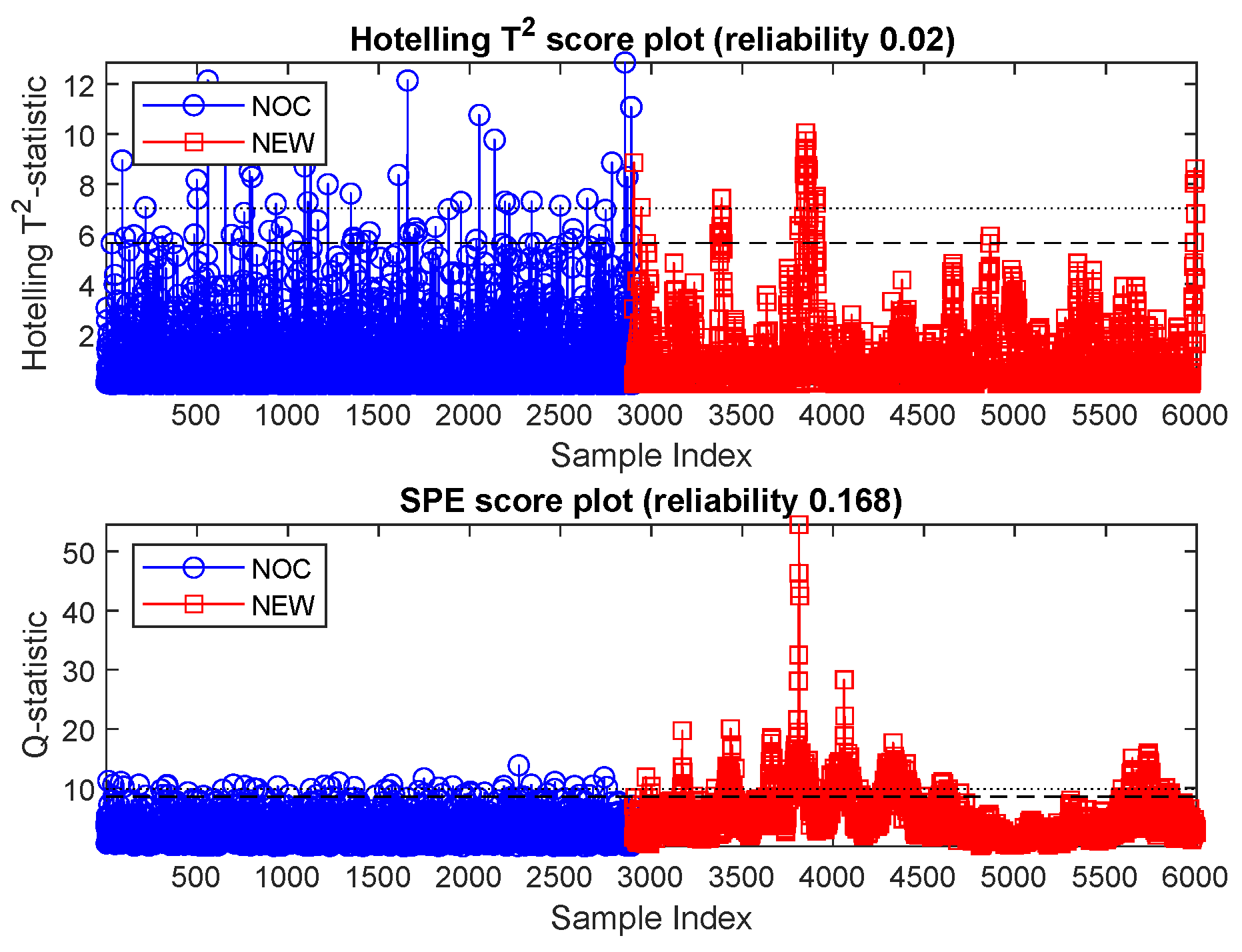
Unlike in Case Study 2, the IF model performed markedly better than the principal component model, as Hotelling’s T² and Q-statistics could collectively identify only 18% of the new data as out-of-control. The performance of this model, based on five principal components capturing in excess of 80% of the variance in the data, is shown in Figure 16. The NOC and the new data were not linearly separable, in contrast to the data in the previous case study, which would explain the disparities in the performance of the PC and IF models.

6. Discussion

In this study, isolation forests were used as a basis for monitoring mineral process operations and compared with principal component models that are widely established in the process industries. Isolation forests are machine learning models designed to identify nonlinear relationships in data through recursive partitioning of the data space. Like most machine learning models, they can do so potentially very reliably in conventional applications, provided that the new data are statistically similar to the data that they had been trained on.

In this investigation, they were used to learn representations of NOC data instead, allowing them to extrapolate to test data markedly different from the data that they had been trained on. This is based on the assumption that at least some of the partitions are complementary to the partitions containing the actual training data and that, generally, these would be partitions associated with training data not considered representative of normal operating conditions.

All the models were designed to minimize type I errors or false positive errors during construction on the NOC data. The control limits of the principal component models were fitted to the NOC data, while the isolation forest threshold for anomaly scores was likewise set to identify 5% of the NOC data as anomalies or OOC data. The threshold at which these probabilities were set to indicate OOC data were tuned on the NOC data to yield an approximately 5% error, similar to what was established for the isolation forest and principal component models.

Future work will include more advanced variants of isolation forests as well as an investigation of the efficacy of isolation forests in process monitoring systems when dealing with larger and higher-dimensional data sets.

7. Conclusions

The following conclusions can be drawn from this investigation:

• In all the case studies used in the analysis, the ability of the models to identify OOC data were assessed, subject to a 5% false-positive rate constraint. The IF models performed better than traditional MSPM models based on principal components in the SAG circuit case study, which showed complex nonlinear dynamics.
• In the case of the coal flotation data set, the OOC clusters were near-linearly separable from the IC data, and the performance of the PCA and IF models was approximately similar.
• In the case of the PGM froth features data set, where the OOC clusters were linearly separable from the IC data, the IF performed reasonably well, but not as well as the principal component models.
• Overall, the IF models were robust, and control of the false positive rate on independent test data could be satisfactorily controlled by setting the contamination factor of the IF to the desired level on the training data.

The results of this study indicate the IFs can be used as a basis for unsupervised monitoring of complex process operations characterized by large sets of operational variables with nonlinear relationships.