Conversion of Induced Polarization Data and Their Uncertainty from Time Domain to Frequency Domain Using Debye Decomposition

Abstract

The time-domain (TD) induced polarization (IP) method is used as an extension of direct current (DC) resistivity measurements to capture information on the ability of the subsurface to develop electrical polarization. In the TD, the transient voltage decay is measured after the termination of the current injection. To invert tomographic TD IP data sets into frequency-domain (FD) models of complex electrical resistivity, a suitable approach for converting TD IP transients and their corresponding uncertainties into the FD is essential. To apply existing FD inversion algorithms to TD IP measurements, a conversion scheme must transform the measured decay curves into FD impedances and also propagate the corresponding measurement uncertainty from the TD to the FD. Here, we present such an approach based on a Debye decomposition (DD) of the decay curve into a relaxation-time distribution and the calculation of the equivalent spectrum. The corresponding FD data error can be obtained by applying error propagation through all of these steps. To accomplish the DD we implement a non-linear Gauss–Newton inversion scheme. We test the conversion scheme in a synthetic study and demonstrate its application to field data on a tomographic TD IP data set measured on the Maletoyvaemskoie ore field (Kamchatka, Russia). The proposed conversion scheme yields accurate impedance data for relaxation processes, which are resolved by the TD measurements. The error propagation scheme provides a reasonable FD uncertainty estimate, as confirmed by a Monte Carlo analysis of the underlying parameter distributions.

1. Introduction

In geoelectrics, the time-domain induced polarization (TD IP) method is used as an extension of direct current (DC) resistivity measurements to capture information on the ability of the subsurface to develop electrical polarization. Theoretical concepts fundamental to the IP method have been studied over the past few decades, primarily motivated by the method’s application to mineral and reservoir characterization (e.g., [1,2,3,4,5,6,7]). Although many field-scale IP measurements are conducted in the time domain (TD), the lithological, textural, and hydraulic properties of the targeted rock have been found to relate especially to the spectral characteristics of the IP phenomenon in numerous frequency-domain (FD) laboratory studies (e.g., [8,9,10,11,12,13,14]). In the context of increasing the measurement accuracy of laboratory and field instruments and emerging FD IP analysis approaches in terms of complex resistivity, the petrophysical and hydrogeophysical communities have started to establish the diagnostic potential of the IP method in their research fields (e.g., [9,15,16,17,18,19]). Independent of the specific application at hand, accurate conversion between TD IP and FD IP data is essential to exploit the FD information contained in TD IP measurements in a quantitative manner. An accurate conversion provides the possibility to draw quantitative conclusions from the FD characteristic of the IP phenomenon with regard to the petrophysical parameters of interest. Therefore, taking extra effort to ensure an accurate and stable conversion of the data set is sensible.

Analytical representations of TD transients can be converted to the FD via the Fourier and Laplace transforms. Specifically, in the conversion of TD IP measurements using standard instrumentation, one faces the problem of sparsely sampled signals, which are typically discretized at 20 time steps or less. To ensure a stable conversion, even with noisy transients, adequate assumptions on their expected shape must be made and included in the conversion. Care must be taken in formulating these assumptions since the use of unsuitable or under-parameterized models can lead to a misrepresentation of the transients and subsequent errors in the conversion. During tomographic inversions of electrical data in the TD and FD, data points are often weighted with their respective errors (e.g., [20,21]). Given individual error estimates for the transients, adequate error propagation through the conversion scheme to the corresponding FD error estimates is therefore essential.

For the conversion of TD IP data sets to the FD, previous studies (e.g., [3,22,23]) have used the assumption of a frequency-independent, constant phase angle (CPA), finding it to be a valid approximation for many laboratory and field applications. As quantitative applications of TD IP measurements call for increasingly high precision, and measurement systems continue to improve, the limitations of the CPA approximation become relevant and must be overcome to fully utilize the quantitative diagnostic potential of the TD IP method. Using a parameterization of the FD complex resistivity in terms of the empirical Cole–Cole model, other studies [24,25,26,27] have been able to invert TD IP data for the spatially distributed spectral behavior of electrical properties in the subsurface. Given scenarios for which the assumption of a Cole–Cole-like behavior is valid, this inversion approach yields easy-to-interpret tomographic results and provides the possibility of relating imaged Cole–Cole parameters to petrophysical properties using relations established in laboratory experiments (e.g., [28]). A drawback of the approach is the Cole–Cole model’s limitation with respect to the possible complexity of the FD characteristics it can represent such as the superposition of multiple polarization processes or spectral characteristics that appear asymmetric in log-log plots in general.

In this work, we describe a general-purpose approach for converting tomographic TD IP data sets to the FD. Importantly, the approach also provides the possibility to accurately propagate a TD data error estimate to a corresponding FD error estimate. The TD to FD conversion scheme presented in this paper is based on the concept of Debye decomposition (DD) (e.g., [29,30,31]). The DD can fit various types of TD transients while including very few prior assumptions on their shape. A measured TD transient is decomposed into a number of exponential decays. The decomposition is performed on a grid of predefined relaxation times. Using an inversion approach, the appropriate contribution of each exponential decay to the superposition can be determined, yielding a relaxation-time distribution (RTD). Related by the Laplace transform, equivalent formulations of the Debye decomposition exist in the TD and FD. The FD response can be calculated from the RTD. Martin et al. [32] demonstrated this equivalence by performing the Debye decomposition on TD and FD IP data sets obtained for the same samples. They found that the estimated RTDs were mostly in agreement with each other, attributing deviations to limitations in TD IP data quality. After converting each transient to the FD, we use a tomographic FD inversion code to compute subsurface images of the complex electrical resistivity at single frequencies.

This work is structured as follows. After a short recap of the theoretical background underlying the Debye decomposition, we formulate the inverse problem inherent in TD to FD conversion. The inverse problem is solved using parameter optimization. We describe the optimization algorithm and explain our choices for the hyperparameters. In a synthetic validation study, we investigate the accuracy and limitations of the TD to FD conversion scheme, complemented by a validation of the error propagation scheme. We conclude with a demonstration of the overall approach on a tomographic TD IP field data set.

2. Time-Domain to Frequency-Domain Conversion of Induced Polarization Data

2.1. Induced Polarization in the Time Domain

During a TD IP measurement, the transient voltage decay $V\left(t\right)$ between the potential electrodes is measured as a function of time t after the termination of the current injection. After an abrupt decrease in the voltage from its primary value $V_0$, associated with the DC resistivity measurement to a secondary value $V_1$, the voltage decreases continuously:

$$\begin{array}{c}\hfill \underset{t\stackrel{}{\to }\infty }{lim}V\left(t\right)=0.\end{array}$$

(1)

Normalization with respect to the primary voltage gives the normalized IP transient $\eta \left(t\right)=\frac{V\left(t\right)}{V_0}$. The ratio of the initial voltage drop at the end of the current injection $t=0$ is known as the chargeability [2]. The occurrence of this electrical relaxation phenomenon is an expression of the subsurface’s ability to develop electrical polarization under an applied electric field.

2.2. Debye Decomposition

The Debye decomposition (DD) is a semi-phenomenological model with the ability to represent various types of electrical relaxation responses based on the superposition of individual Debye responses. We adopted and modified the FD forward operator of the DD after Nordsiek and Weller [31]:

$$\begin{array}{c}\hfill \widehat{Z}\left(\omega \right)=R_0-\sum _{k=1}^M{\gamma }_k\left(1-\frac{1}{1+i\omega {\tau }_k}\right),\end{array}$$

(2)

where M is the number of Debye terms, $\omega$ is the angular frequency, and $i^2=-1$ is the imaginary unit. These parameters were used to calculate the spectrum of the complex electrical impedance $\widehat{Z}\left(\omega \right)$, which is equivalent to the measured TD transient. The relaxation time ${\tau }_k$ is the characteristic time constant of the k-th Debye term. The DC resistance $R_0$ is the magnitude of the electrical impedance at the low-frequency limit of the spectrum:

$$\begin{array}{c}\hfill R_0=\underset{\omega \stackrel{}{\to }0}{lim}\left|\widehat{Z}\left(\omega \right)\right|.\end{array}$$

(3)

The parameters ${\gamma }_k$ have the unit of resistance and scale the contributions of the different Debye terms to the superposition. By choosing ${\gamma }_k$ as scaling parameters and thus deviating from the formulation of Nordsiek and Weller [31], we avoid correlated errors between the different Debye terms in the superposition. Plotting the values of ${\gamma }_k$ against the corresponding relaxation times ${\tau }_k$ yields the RTD.

We estimate the values of ${\gamma }_k$ by inverting the measured TD transient on a grid of predefined relaxation times ${\tau }_k$ using the TD forward operator, which is equivalent to Equation (2) (e.g., [30,33,34]):

$$\begin{array}{c}\hfill \eta \left(t\right)=\frac{1}{R_0}\sum _{k=1}^M{\gamma }_{k}exp\left(-\frac{t}{{\tau }_k}\right).\end{array}$$

(4)

A closer investigation of Equation (2) shows that it is reasonable to restrict the interpretation of the derived spectrum to the angular frequencies $\frac{1}{{\tau }_{max}}<\omega <\frac{1}{{\tau }_{min}}$, which assumes that there is a smallest relaxation time ${\tau }_{min}$ and a largest relaxation time ${\tau }_{max}$ that can be resolved with a given measurement. In this work, we chose ${\tau }_{min}$ and ${\tau }_{max}$ to be equal to the first and last time values used for the discretization of the transient.

2.3. Formulation of the Inverse Problem

The goal of the DD is to decompose a measured TD transient into an RTD. We do not use the discrete values of the normalized TD transient as data since their errors are correlated due to division by the measured quantity $V_0$. Instead, we choose

$$\begin{array}{c}\hfill \mathbf{d}=R_0{\left({\eta }_1,\dots ,{\eta }_i,\dots ,{\eta }_N\right)}^T,\end{array}$$

(5)

at discrete time steps

$$\begin{array}{c}\hfill \mathbf{t}={\left(t_1,\dots ,t_i,\dots ,t_N\right)}^T,\end{array}$$

(6)

which provides us with uncorrelated measurements to invert. In the model domain, the inverse problem is discretized on a grid of M predefined, ${log}_{10}$-spaced, relaxation times ${\tau }_k$. It is critical that the model domain discretization covers a wide enough parameter range and provides enough degrees of freedom. With the first and last time steps of the discretized transient being $t_1$ and $t_N$, we choose ${\tau }_k\in [{10}^{{log}_{10}\left(t_1\right)-1.5},{10}^{{log}_{10}\left(t_N\right)+1.5}]$, extending the discretization of the model domain by 1.5 decades to the left and right of the sampled time frame. The number of relaxation times M is based on the number of decades covered by the model-domain discretization so that the density of the model-domain discretization is consistent for differently sampled transients. For each decade in ${\tau }_k$, we use 25 relaxation times for the discretization of the model domain, which is 5 relaxation times more than the 20 per decade recommended by Weigand and Kemna [35], ensuring enough degrees of freedom. To account for the wide range of values within ${\gamma }_k$ and to restrict the inversion from yielding results associated with ${\gamma }_k<0$, the natural logarithms of ${\gamma }_k$ are used as the model parameters:

$$\begin{array}{c}\hfill \mathbf{m}={\left(ln\left(\frac{{\gamma }_1}{{\gamma }_0}\right),\dots ,ln\left(\frac{{\gamma }_k}{{\gamma }_0}\right),\dots ,ln\left(\frac{{\gamma }_M}{{\gamma }_0}\right)\right)}^T.\end{array}$$

(7)

Note that the division by ${\gamma }_0=1\Omega$ is necessary to ensure that the argument of $ln(·)$ is dimensionless. For simplicity, this is implied in the notation $ln\left(\frac{{\gamma }_k}{{\gamma }_0}\right)=ln\left({\gamma }_k\right)$ from here on. The TD forward operator of the DD is modified as

$$\begin{array}{c}\hfill \widehat{Z}\left(t\right)=\sum _{k=1}^{M}exp\left(ln\left({\gamma }_k\right)-\frac{t}{{\tau }_k}\right),\end{array}$$

(8)

leading to the discrete TD forward operator (e.g., [36])

$$\begin{array}{c}\hfill f_i(\mathbf{m},t_i)=\sum _{k=1}^M{G}_{ik}exp\left(m_k\right),\end{array}$$

(9)

with

$$\begin{array}{c}\hfill G_{ik}=exp\left(-\frac{t_i}{{\tau }_k}\right).\end{array}$$

(10)

Setting up the forward operator as a matrix-vector multiplication is favorable in terms of computational performance due to the possibility of parallel computing. Note that we formulate $\mathbf{f}(·)$ as a function of $\mathbf{m}$ and $\mathbf{t}$. In most cases, $\mathbf{t}=\mathrm{const}$. The only exception is in Section 2.4, where we discuss the stacking of subsequent injection pulses for a given model realization; hence. $\mathbf{m}=\mathrm{const}$. From here on we only explicitly pass the argument to the forward operator that is not constant.

The inverse problem that results from Equation (9) is non-linear. The corresponding cost function

$$\begin{array}{c}\hfill \mathsf{\Psi }\left(\mathbf{m}\right)=\frac{1}{2}{\left(\mathbf{d}-\mathbf{f}\left(\mathbf{m}\right)\right)}^T{\mathbf{C}}_D^{-1}\left(\mathbf{d}-\mathbf{f}\left(\mathbf{m}\right)\right)+\frac{1}{2}\lambda {\mathbf{m}}^T\mathbf{R}\mathbf{m},\end{array}$$

(11)

is minimized iteratively using a pseudo-Newton model update, as described in Tarantola [37]:

$$\begin{array}{c}\hfill {\mathbf{m}}_{q+1}={\mathbf{m}}_q+\alpha \Delta \mathbf{m}={\mathbf{m}}_q-\alpha {\left({\mathbf{J}}_{TD}^T{\mathbf{C}}_D^{-1}{\mathbf{J}}_{TD}+\lambda \mathbf{R}\right)}^{-1}\left({\mathbf{J}}_{TD}^T{\mathbf{C}}_D^{-1}\left(\mathbf{f}\left({\mathbf{m}}_q\right)-\mathbf{d}\right)+\lambda \mathbf{R}{\mathbf{m}}_q\right).\end{array}$$

(12)

The Jacobian and the step length are represented by ${\mathbf{J}}_{TD}$ and $\alpha$, respectively. Since the inverse problem is underdetermined, regularization $\lambda >0$ has to be applied to ensure that $\left({\mathbf{J}}_{TD}^T{\mathbf{C}}_D^{-1}{\mathbf{J}}_{TD}+\lambda \mathbf{R}\right)$ can be inverted. We use a roughness operator $\mathbf{R}$ that minimizes the squared difference between the model parameters of the neighboring Debye terms. The strength of the applied regularization is controlled by the parameter $\lambda$. Measurement uncertainties are accounted for in the data-precision matrix ${\mathbf{C}}_D^{-1}$. The root-mean-square error (RMSE)

$$\begin{array}{c}\hfill \epsilon =\sqrt{\frac{{\left(\mathbf{d}-\mathbf{f}\left(\mathbf{m}\right)\right)}^T{\mathbf{C}}_D^{-1}(\mathbf{d}-\mathbf{f}\left(\mathbf{m}\right))}{N}}\end{array}$$

(13)

is used to estimate the goodness of the data fit achieved by a given model realization in the context of measurement uncertainties. For each iteration, the step length $\alpha$ is optimized automatically using a line-search approach described in Kemna [38]. During the line search, three trial-model updates are calculated for ${\alpha }_{trial}\in \{0,\alpha /2,\alpha \}$ and their corresponding data fits $\epsilon$ are evaluated. The updated step length is then chosen as the minimum of a parabola fitted through $\epsilon \left({\alpha }_{trial}\right)$. The inversion is terminated if the norm of the model update $|\Delta \mathbf{m}|$ vanishes, indicating that the maximum a posteriori (MAP) solution has been found.

2.4. Adaptation to Common Data-Acquisition Strategies

Most TD IP measurement systems use gate integration during the measurement in order to reduce high-frequency noise. This means that the transient returned by the instrument is actually a sequence of mean values, each of which is calculated for a corresponding time gate. Different choices can be made for the widths of the time gates. Given the case where the widths of the time gates increase in a ${log}_{10}$ manner, Fiandaca et al. [25] suggested using the center of the time gates, calculated using the geometric mean, as the time points to represent the averaged values in the transient. Since this resolves the problem of adjusting the forward operator to the gate integration, we use transients sampled at ${log}_{10}$-spaced time steps.

During a TD IP measurement, a sequence of opposing current pulses is injected into the subsurface. The measured TD transient is calculated as the mean of the transients induced by these pulses to increase the signal-to-noise ratio. For a given model realization $\mathbf{m}=\mathrm{const}$, the forward operator has to be extended as (e.g., [25,34])

$$\begin{array}{c}\hfill {\mathbf{f}}_{{\mathrm{Stack}}_j}\left(\mathbf{t}\right)=\sum _{m=1}^j\sum _{k=1}^2{(-1)}^{m+k}\mathbf{f}\left(\mathbf{t}+\mathbf{1}(k-1)T_{\mathrm{On}}+\mathbf{1}(j-m)(T_{\mathrm{On}}+T_{\mathrm{Off}})\right)\end{array}$$

(14)

and

$$\begin{array}{c}\hfill {\mathbf{f}}_A\left(\mathbf{t}\right)=\frac{1}{N_{\mathrm{Stacks}}}\sum _{j=1}^{N_{\mathrm{Stacks}}}{(-1)}^{j+1}{\mathbf{f}}_{{\mathrm{Stack}}_j}\left(\mathbf{t}\right),\end{array}$$

(15)

where $\mathbf{f}(·)$ represents the forward calculation given in Equation (9), ${\mathbf{f}}_{{\mathrm{Stack}}_j}$ represents the j-th transient with the superposition of the transients from prior injection pulses taken into account, and ${\mathbf{f}}_A$ is the averaged transient after $N_{\mathrm{Stacks}}$ stacks. We use the formulation in Equation (15) to adjust the forward calculation $\mathbf{f}(·)\leftarrow {\mathbf{f}}_A(·)$ appropriately when dealing with stacked transient data.

3. Uncertainty Approximation and Propagation

Choosing a suitable regularization strength is essential for the conversion, as well as the error propagation from the TD to the FD. In our work, we base the choice of an appropriate regularization strength on $\epsilon$, assuming that we have a good estimate of the data uncertainty. We choose the regularization strength in such a way that the MAP solution achieves $\epsilon =1$, fitting the measurements appropriately in the context of their respective uncertainties (e.g., [20,38,39]). Details of our approach for finding the optimal regularization strength ${\lambda }_{final}$ can be found in Appendix A. The analytical propagation of measurement errors from the TD to the FD is based on an adequate uncertainty characterization in the model domain. Here, $\lambda \mathbf{R}$ can be identified as the precision matrix of the prior term. Assuming normally distributed model-parameter uncertainties near the MAP solution, the posterior covariance matrix [37]

$$\begin{array}{c}\hfill {\mathbf{C}}_M={\left({\mathbf{J}}_{TD}^T{\mathbf{C}}_D^{-1}{\mathbf{J}}_{TD}+\lambda \mathbf{R}\right)}^{-1},\end{array}$$

(16)

is approximated from the result of the inversion. It can be used as an uncertainty measure for the estimated model parameters, considering both the measurement uncertainty and prior uncertainty. Using error propagation, the following formulation can be used for the mapping of the data errors to the model domain [40]:

$$\begin{array}{c}\hfill {\mathbf{C}}_E={\mathbf{C}}_M{\mathbf{J}}_{TD}^T{\mathbf{C}}_D^{-1}{\mathbf{J}}_{TD}{\mathbf{C}}_M.\end{array}$$

(17)

Equation (17) isolates the propagated uncertainty of the inverted measurements and is, therefore, the approximation used for the error propagation from the TD to the FD. The Jacobian of the FD response can be calculated from the partial derivatives with respect to the model parameters $ln\left({\gamma }_k\right)$. For the k-th model parameter, we find

$$\begin{array}{c}\hfill {\mathbf{J}}_{FD,k}={\left(\begin{array}{cc}\frac{\partial Z^{\prime }\left(\omega \right)}{\partial ln\left({\gamma }_k\right)}& \frac{\partial Z^{″}\left(\omega \right)}{\partial ln\left({\gamma }_k\right)}\end{array}\right)}_k^T={\left(\begin{array}{cc}-{\gamma }_k\frac{{\left(\omega {\tau }_k\right)}^2}{1+{\left(\omega {\tau }_k\right)}^2}& -{\gamma }_k\frac{\omega {\tau }_k}{1+{\left(\omega {\tau }_k\right)}^2}\end{array}\right)}_k^T,\end{array}$$

(18)

for the formulation in terms of the real and imaginary parts. The covariance matrix for the real and imaginary parts is calculated from ${\mathbf{J}}_{FD}$ and ${\mathbf{C}}_E$ while also accounting for the uncertainty of $R_0$:

$$\begin{array}{c}\hfill \mathbf{cov}(Z^{\prime },Z^{″})=\mathrm{var}\left(R_0\right)\left(\begin{array}{cc}1& 0\\ 0& 0\end{array}\right)+\left({\mathbf{J}}_{FD}{\mathbf{C}}_E{\mathbf{J}}_{FD}^T\right).\end{array}$$

(19)

From the covariance matrix of the real and imaginary parts, the covariance matrix of the logarithmic magnitude and phase can be obtained according to:

$$\begin{array}{c}\hfill \mathbf{cov}(ln\left|Z\right|,\varphi )=\left(\begin{array}{cc}\frac{\partial ln\left|Z\right|}{\partial Z^{\prime }}& \frac{\partial ln\left|Z\right|}{\partial Z^{″}}\\ \frac{\partial \varphi }{\partial Z^{\prime }}& \frac{\partial \varphi }{\partial Z^{″}}\end{array}\right)\mathbf{cov}(Z^{\prime },Z^{″}){\left(\begin{array}{cc}\frac{\partial ln\left|Z\right|}{\partial Z^{\prime }}& \frac{\partial ln\left|Z\right|}{\partial Z^{″}}\\ \frac{\partial \varphi }{\partial Z^{\prime }}& \frac{\partial \varphi }{\partial Z^{″}}\end{array}\right)}^T.\end{array}$$

(20)

4. Synthetic Validation Study

4.1. Accuracy of the TD to FD Conversion

To investigate the accuracy of the approach described above when extracting information at a frequency of 1 Hz, we tested it on 30 synthetic transients with varying relaxation times

$$\begin{array}{c}\hfill d\left(t_i\right)=\frac{R_0{V}_1}{V_0}exp\left(-\frac{t_i}{{\tau }_s}\right),\end{array}$$

(21)

with $R_0=1 \Omega$, $\frac{V_1}{V_0}=0.1$, and ${\tau }_s\in [{10}^{-2},10]$s. The synthetic transients were discretized over 20 time gates, with geometric means $t_i$ that were ${log}_{10}$-spaced between $0.1$s and $1$s. Noise with a relative error of $1\%$ and an absolute error of ${10}^{-6}\Omega$ was added to the synthetic measurements. The pseudo-random number generator was initialized with the same seed for all synthetic transients so that the added noise realization was always the same. During the Debye decomposition, the standard deviation of the synthetic noise was accounted for by modification of the data-precision matrix ${\mathbf{C}}_D^{-1}$. During the inversion of all synthetic transients, the regularization strength was adapted to the data uncertainty to achieve a data fit of $\epsilon =1$. We evaluated the accuracy of the conversion by investigating its ability to estimate the phase of the complex electrical impedance, the results of which are shown in Figure 1. The expected phase value for a given synthetic transient is calculated analytically. Although the misfit between the expected phase and estimated phase is high for the conversion of very fast relaxation processes, the estimation is exact if the relaxation time ${\tau }_s$ of the synthetic transient lies within the sampled time frame from $0.1$s to $1$s. For slower relaxation processes, the accuracy of the conversion does not drop as drastically as it does for faster relaxation processes. Up to a relaxation time of ${\tau }_s=10$s, a good estimation of the phase is possible through the extrapolation of the information contained in the synthetic measurements. The achieved data fits $\epsilon$ were all close to the target value of $\epsilon =1$, as shown in Figure 1. The optimized regularization strength ${\lambda }_{final}$ was minimal for synthetic transients with relaxation times within the sampled time frame. Here, the inversion was dominated by the measurements. For values of ${\tau }_s$ outside the sampled time frame, the inversion was dominated by the prior information, which corresponded to higher estimates of ${\lambda }_{final}$.

4.2. Validation of Error Propagation

The error propagation from the TD to the FD was based on the existence of a suitable covariance matrix for describing the estimated RTDs’ uncertainty. Equation (17) provides such an estimate for the mapping of the data errors to the model domain, assuming normal data error and model-parameter distributions. To validate the error propagation from the TD to the model domain, we created ${10}^4$ noise realizations of Equation (21) with $\frac{V_1}{V_0}=0.1$, ${\tau }_s=0.5$s, and $R_0=1\Omega$, as exemplarily shown in Figure 2. The error on $R_0$ was simulated by adding a synthetic noise realization with a $10\%$ relative error and a $5\times {10}^{-3}\Omega$ absolute error to $R_0$. The synthetic transient was discretized over 20 ${log}_{10}$-spaced time gates with geometric means $t_i$ between $0.1$s and $1$s to create the synthetic measurements. The noise added to the synthetic transient had a relative error of $1\%$ and an absolute error of ${10}^{-6}\Omega$. Inversions were performed with a fixed regularization strength, meaning that variations in the cost function (11) only occurred in the data misfit term and not in the prior term, isolating the scatter in the estimated model parameters that was caused by the noise on the synthetic measurements. Because the discretization at 20 time steps only provided a limited sample of the noise, and the regularization strength was not adapted to the specific noise realization, the achieved values for $\epsilon$ showed a scatter. The regularization strength was chosen to be $\lambda =1$, yielding scattering $\epsilon$ values with a mean $\overline{\epsilon }\approx 1$.

The synthetic validation study showed that although the distributions of the model parameters deviated from the normal distribution, they were otherwise well-behaved (see Figure 2 for an example of a model parameter). The distributions of the model parameters obtained during the synthetic study were used to calculate the reference covariance matrix and to validate the choice of the uncertainty estimator in the model domain, which was used for the error propagation and calculated according to Equation (17). Figure 3 shows a comparison of the reference matrix calculated from the scatter of the model-parameter estimates and the approximations of ${\mathbf{C}}_M$ and ${\mathbf{C}}_E$ using Equations (16) and (17), which were calculated from the inversion result of the noise-free decay. As expected, ${\mathbf{C}}_M$ showed strong deviations from the reference matrix since it included the uncertainty of the prior information and did not isolate the mapping of the data errors to the model domain. The matrix ${\mathbf{C}}_E$ was a much better approximation of the reference matrix. However, although it captured the overall shape, ${\mathbf{C}}_E$ also showed deviations from the reference matrix. These can be traced back to the assumption of normally distributed model-parameter estimates underlying Equation (17), which was violated in some cases, as shown in Figure 2. We, therefore, assumed ${\mathbf{C}}_E$ to be a valid but not completely exact approximation of the uncertainty in the model domain. To investigate the distributions of the FD estimates, the FD responses of all ${10}^4$ RTDs were calculated at 1 Hz, and are shown in Figure 2. The distributions of $ln\left|Z\right|$ and $\varphi$ were not normal but were well-behaved.

The scatter of the FD responses calculated using the inversion results with $\lambda =1$ was used to estimate the reference standard deviation for the individual components of the FD estimates. To validate the accuracy achieved by the error propagation scheme, we performed a conversion for ${10}^3$ noise realizations, for which we adapted $\lambda$, calculated the FD error estimate for each FD estimate, and compared the mean of the error estimates to the reference. Figure 4 shows the distributions of the estimated standard deviations for the different components of the FD estimates. The standard deviations of both $ln\left|Z\right|$ and $\varphi$ were well estimated by the proposed error propagation scheme.

5. Demonstration of the Application to Tomographic Field Measurements

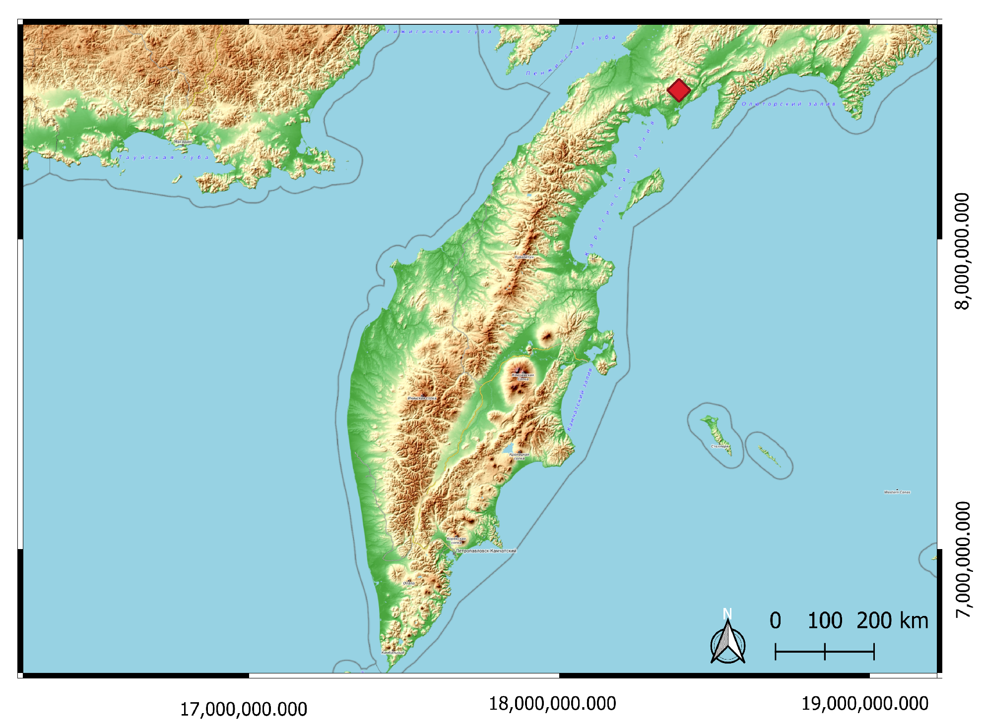
We demonstrated the application of the new conversion approach to tomographic field measurements on a TD IP data set that was measured in the Maletoyvaemskoie ore field (MOF), located in the central part of the Maketoyvaemskoie ore cluster in the North Kamchatka region (Russia, compare Figure 5). Geologically, the field site is located in the central part of a volcanic-tectonic structure that represents a stratovolcano. The stratovolcano is located within the Koryak-Central Kamchatsky belt of the Neogen-Quaternary age and is composed of Early Miocene stratified volcanic and sedimentary rocks (effusive, pyroclastic, and tuff-sedimentary rocks predominantly of Andesitic composition) with different degrees of hydrothermal and metasomatic alteration. The MOF includes three gold objects considered small HS (high sulfidation)-type gold deposits (Yugo-Zapadnoye, Gaching, and Yubileinoye), several gold anomalies superimposed with copper-arsenic sulfosalt mineralization, and copper anomalies [41,42]. Most of the discovered ore bodies are of high chargeability (e.g., [43]). The MOF features massifs of secondary quartzites with pronounced horizontal zonality, which are typical for HS-type deposits. Epithermal gold deposits of HS type are the new types of deposits found in the far east of Russia. To date, only a few economically important HS deposits have been discovered within the region. They are settled within young volcano-sedimentary belts, where hydrothermally altered (advanced argillic) rocks have formed due to the aside alteration of initial rocks by hydrothermal processes within active hydrothermal systems, surrounding the gold HS deposits. Numerous fields of altered rocks have been discovered within the Kamchatka peninsula, being potential sources of high-grade and large-tonnage epithermal gold-silver and copper-porphyry deposits. Starting in the year 2000, gold prospecting was carried out in the MOF.

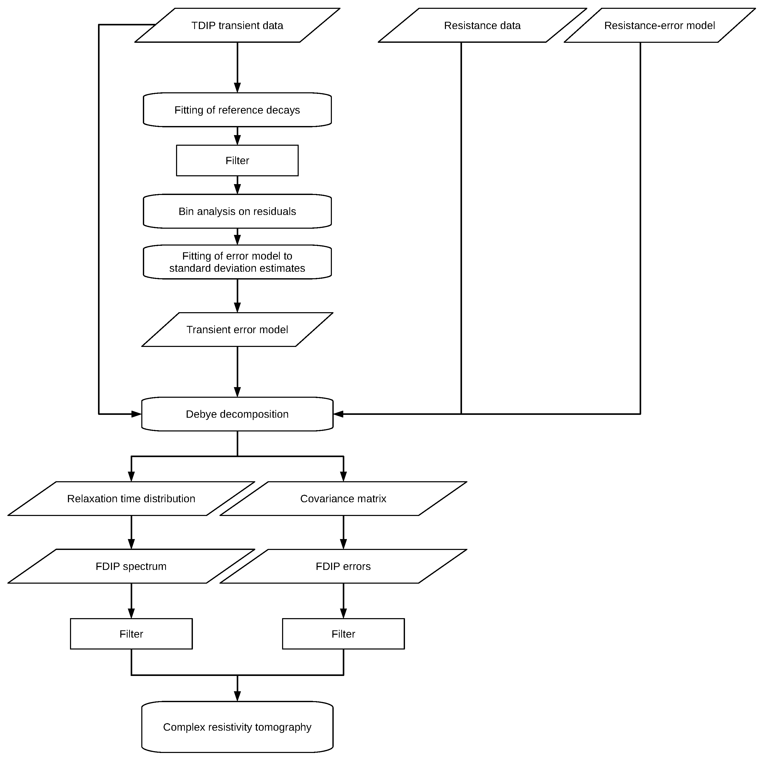
There have been significant efforts to characterize the field site using geophysical and petrophysical surveys. Geoelectric measurements have been complemented by information from other geophysical methods, such as geomagnetic measurements, and geological surveys. Gurin [43] presented the results and interpretations of multiple geophysical and petrophysical surveys carried out between 2016 and 2017 in the central part of the MOF. The IP characteristics of the field site have been previously analyzed (e.g., [44]). The extensive studies that have been conducted in the area provide the basis on which the validity of our results, obtained from the conversion and subsequent tomographic inversion of the TD IP data, can be assessed. The TD IP data set was obtained using pole-dipole measurements, which were carried out along a 2400 m long profile, utilizing an injection and off-time of 1 s and a total of 15 stacks. A potential dipole with an electrode separation of $20$m was used while the current electrode was moved on a $100$m grid. The second current electrode, assumed to be located at an infinite distance during the tomographic inversion, was placed $3500$m away from the nearest point on the profile. For data acquisition, an AIE-2 instrument was used, featuring a VP-1000 (1 kW power) transmitter and a VP-MPP receiver. No low-pass filter was used during the data acquisition, eliminating the need to correct the early times of the transients for the corresponding effects. The workflow we followed during the processing of the tomographic TD IP field data set is presented in Figure 6.

Figure 5. Kamchatka, with the location of the Maletoyvaemskoie ore field indicated in red. Map by OpenStreetMap (OSM) [45]. Coordinate System: WGS 84. A detailed geological map of the field site is provided in Gurin [43].

Figure 5. Kamchatka, with the location of the Maletoyvaemskoie ore field indicated in red. Map by OpenStreetMap (OSM) [45]. Coordinate System: WGS 84. A detailed geological map of the field site is provided in Gurin [43].

Figure 6. Illustration of the workflow followed during the TD IP field-data processing.

Figure 6. Illustration of the workflow followed during the TD IP field-data processing.

To assess the general data quality, filter transients that showed highly erratic behavior, and later quantify errors, we followed Flores Orozco et al. [46] and started the data processing by fitting a power-law model to the measured TD transients. Note that the power-law model

$$\begin{array}{c}\hfill d\left(t_i\right)=a{t_i}^b\end{array}$$

(22)

approximates the TD equivalent of the CPA spectrum of the electrical impedance [3] given by:

$$\begin{array}{c}\hfill \widehat{Z}\left(\omega \right)=R_{0}K{\left(i\omega \right)}^{-b}.\end{array}$$

(23)

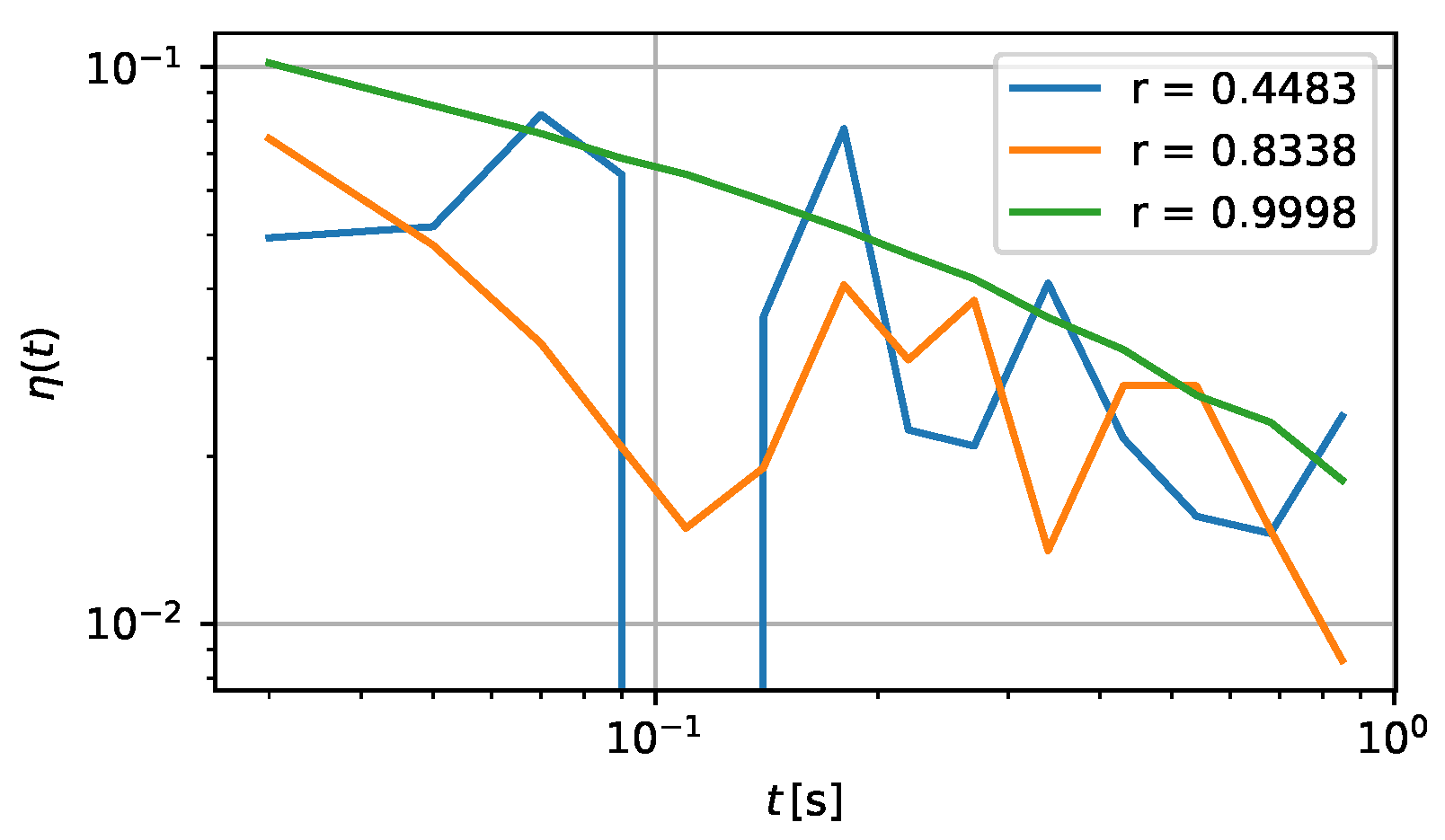
By basing the filtering on the Pearson correlation coefficient between the measured decay and the response of the fitted power-law model, we defined erratic behavior as a strong deviation from the CPA behavior. We excluded transients with $r<0.9$ from the data processing, interpreting them as non-physical. This filter reduced the total size of our data set by $9\%$. Examples of transients and their corresponding Pearson correlation coefficients are shown in Figure 7.

Since the error quantification aimed to characterize the statistical uncertainty of the data, performing it after filtering non-physical transients from the data set was reasonable. Based on the scatter of the measurements around the responses of the fitted power-law models, we estimated the standard deviations of $d_i$ by performing a bin analysis [47]. We calculated the residuals of all $d_i$ readings to the power-law model response and plotted them against the $d_i$ readings themselves. After subdividing the data set into ${log}_{10}$-spaced bins, we estimated the standard deviations corresponding to the different bins from the scatter of the residuals within them. Finally, we fitted a linear error model through the estimated standard deviations, as shown in Figure 8. To account for the varying number of residuals within the different bins, we weighted the estimated standard deviations by $\frac{1}{\sqrt{N_{Bin}}}$ during the fit. The fitted error model was used to estimate the standard deviations of all $d_i$ readings during the TD to FD conversion. To account for the simplicity of the fitted power-law model and allow for more complex RTDs, we slightly adjusted the fitted error model by reducing the absolute error (see Figure 8). For the DC resistances, we used a linear error model with relative and absolute errors of $9\%$ and $5\times {10}^{-3}\Omega$, respectively. Lacking reciprocal measurements, these parameters were chosen conservatively and in such a way that the results of the TD to FD conversion, as well as those of the tomographic inversion, were robust with regard to small changes in the values chosen for the DC error model.

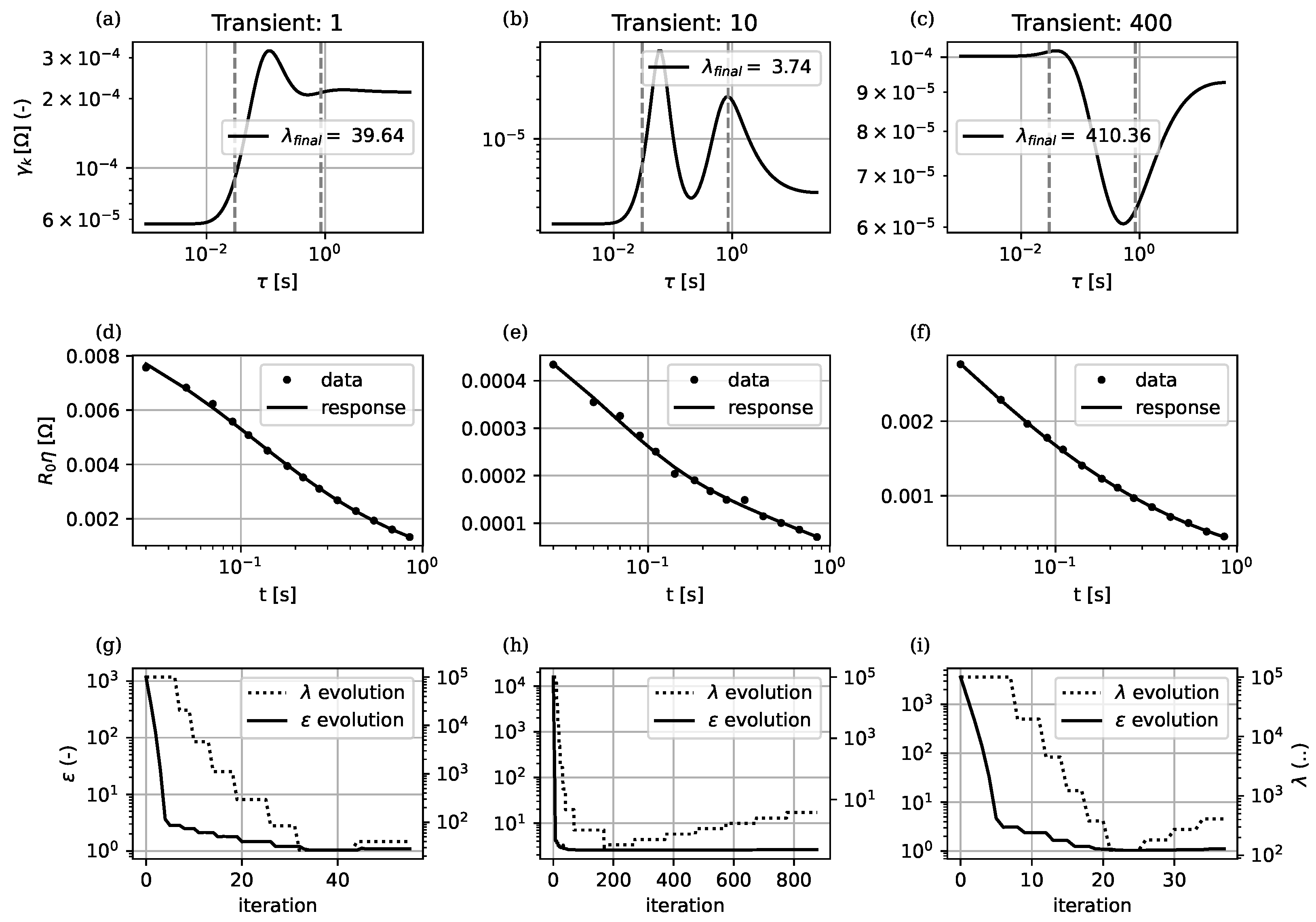
The inversions of all the measured TD transients into RTDs were performed with the adaptation of the regularization strength to the data uncertainty. Figure 9 shows the development of $\epsilon$ and $\lambda$ during the inversion process for the sample transients. All inversions started with a high $\epsilon$ of the starting model, which decreased significantly during the first 10 iterations. Note that the development of $\epsilon$ showed discontinuities in the iterations, at which time the regularization strength $\lambda$ was updated.

The estimated RTDs were of varying complexity, as displayed in Figure 9. Although some showed no or only one peak, others featured multiple peaks and structures that indicated the presence of relaxation phenomena, which could not be quantitatively described by the CPA assumption or single Debye or Cole–Cole terms. Generally, the estimated RTDs achieved good data fits, as shown in Figure 9.

For every converted transient, we extracted electrical impedance data from the FD responses at 1 Hz and 20 Hz and used the magnitude and phase values as input for the tomographic inversions. Prior to the tomographic inversions, we filtered the data set based on the histograms of the apparent resistivity magnitude and phase, as shown in Figure 10, and excluded all measurements associated with geometric factors larger than 50,000. Figure 11 shows the FD error estimates at 1 Hz. We fitted the error models through the data set to demonstrate the systematic behavior of the error estimates. For the phase-error model, we used the inverse power-law relation proposed by Flores Orozco et al. [48]

$$\begin{array}{c}\hfill \mathrm{std}\left(\varphi \right)={a\left|Z\right|}^{-b}+c,\end{array}$$

(24)

whereas for the magnitude-error model, we followed the standard linear assumption, featuring relative and absolute errors. For the tomographic inversion, we used the individual error estimates rather than the ones associated with the fitted-error models. We were unable to obtain stable tomographic inversion results when including data points with phase errors $\mathrm{std}\left(\varphi \right)<1$mrad, so we excluded them. As can be seen from the scatter plot of the phase errors in Figure 11, this mainly corresponded to data points with a high impedance magnitude $\left|Z\right|$, which mainly occurred in our data set for the very shallow region between meters 2000 and 2500 of the profile. Due to the resulting local sparsity of the data points, the tomographic inversion result was less data-driven in that region.

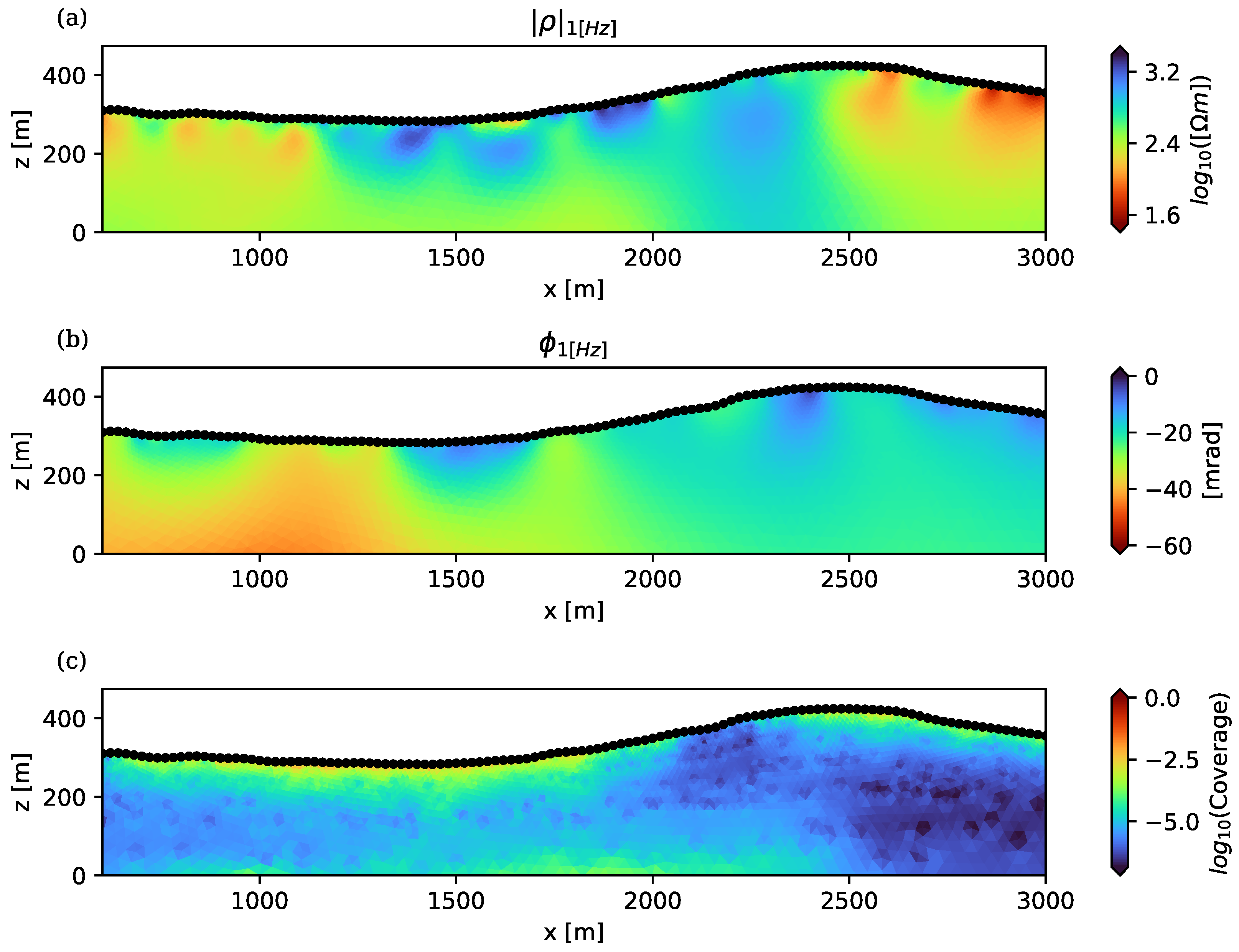
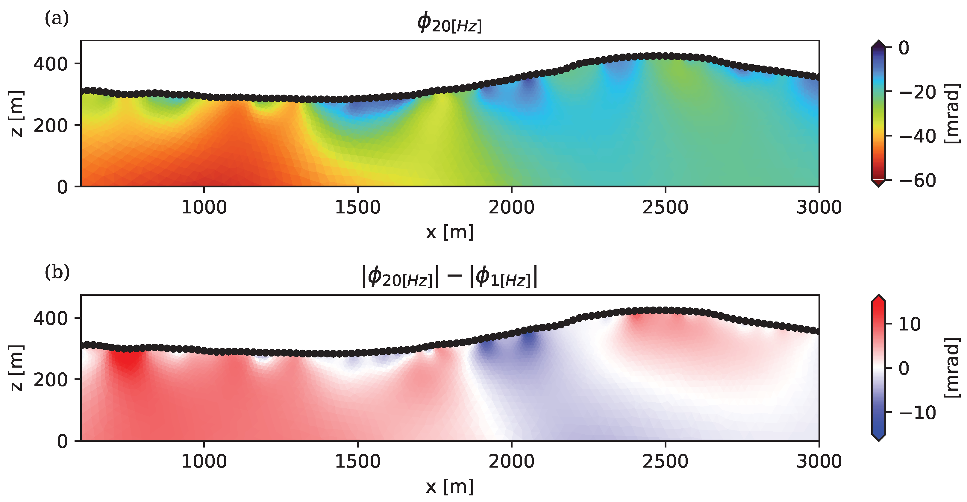
The tomographic inversions were performed using a finite element-based, smoothness-constrained complex resistivity inversion code developed by Kemna [38]. Figure 12 displays the results of the tomographic inversion at 1 Hz, alongside a plot of the estimated coverage, which shows the regions of the model that were less constrained by the measurements. The obtained images of the complex resistivity were realistic, given the expected geological context. The estimated phases achieved values from $0$mrad to $-60$ mrad. Large absolute phase values between $-40$mrad and $-60$mrad were primarily located at the start (left) of the profile and extended up to $1700$m. These large absolute phase values also coincided with larger values of ${\sigma }^{″}$, as shown in Figure 13, which is approximately proportional to the metal factor (e.g., [49,50]) for the phase angles we considered. In contrast to the phase, large absolute values of ${\sigma }^{″}$ can be seen in the region between $2500$m and $3000$m. In the shallow region around $1500$m, a reduction in ${\sigma }^{″}$ occurred. We can attribute this reduction in ${\sigma }^{″}$ near the surface to the presence of quartzites and interpret the large ${\sigma }^{″}$ values at depths from $600$ to $1800$m to be caused by copper-porphyry deposits, located within moderately to strongly sulfidized rocks. With respect to the possible exploration of deposits in the MOF, the described region can be classified as a promising area for potential copper mining. For further information on prospective areas in the MOF deduced from geophysical measurements at the study site, we refer the reader to Gurin [43]. Although the frequency dependence of the magnitude was negligible, the frequency dependence of the phase can be clearly seen from the comparison of the inversion results at $1$Hz and $20$Hz, as displayed in Figure 14. This spectral behavior can be interpreted further, for example, in terms of the associated relaxation times. Assuming a single dominant relaxation process ${\tau }_{peak}$, the difference plot at the bottom in Figure 14 would indicate ${\tau }_{peak}<\frac{1}{2\pi }$s in the red regions and ${\tau }_{peak}>\frac{1}{40\pi }$s in the blue regions. As the radius of ore grains relates to the relaxation time ${\tau }_{peak}$ (e.g., [5,12,51,52]), the spectral characteristics captured by our conversion approach can be interpreted in terms of the expected ore grain size. Furthermore, the spectral behavior displayed in Figure 14 is consistent with our interpretation of the ${\sigma }^{″}$ image (see Figure 13). Note that parts of the blue region in the difference plot coincide with areas of lower coverage (see Figure 12).

6. Discussion

The presented work shows that a quantitative TD to FD conversion of IP transients using Debye decomposition is possible and can be applied to tomographic TD IP data sets. The major precondition for the application of the described approach is the suitability of the DD to describe the polarization process at hand. Other limitations of the approach can be traced back to the limited information content in the TD IP measurements themselves. A symptom of this is the high phase error, caused primarily by the relatively small number of time gates used to discretize the transients, which is often $N=20$ or less for TD IP field instruments. The phase error can be drastically reduced by a more accurate sampling of the transients, with the noise level on the TD transient remaining unchanged. Furthermore, the presented approach is unable to yield accurate FD estimates for relaxation processes that are not resolved by the measurement, as shown in Figure 1. For relaxation processes far beyond the measured time interval, or in the case of highly erratic behavior, our approach can fail to invert a given transient into an appropriate RTD. A prior assessment of a given data set is therefore necessary, forcing the user to make a judgment on whether a quantitative analysis and interpretation of the data set is appropriate or not.

During the error propagation from the TD to the FD, we exclusively focus on statistical errors. As the TD to FD conversion is non-linear, the analytical error propagation is not mathematically exact, and the estimate of the FD uncertainty will always be an approximation of the real error. Numerical approaches may be more suited for exact error propagation, but may potentially increase the computational effort to a level exceeding what is reasonable when applying the conversion to larger-scale tomographic TD IP data sets. For the inversion of a TD transient into an RTD, we set up our algorithm to estimate the natural logarithms of ${\gamma }_k$. This worked well for all the cases we encountered during our work since we avoided negative estimates for ${\gamma }_k$ and achieved a higher consistency in the estimated RTDs. However, the following inconsistencies were introduced with regard to the assumptions underlying the error propagation: We inverted the discrete and linear transients of $d_i$ by minimizing a cost function that assumed they were subject to normal noise. In the model space, we used ${\mathbf{C}}_E$ as a covariance matrix to describe the uncertainty of the estimated model parameters $ln\left({\gamma }_k\right)$, with ${\gamma }_k$ and $d_i$ both having the unit of resistance. This is mathematically inexact since $ln\left({\gamma }_k\right)$ and $d_i$ cannot both be normally distributed. The same inconsistency arose in the conversion from the model domain to the FD. Still, the presented synthetic validation study suggests that the propagated FD uncertainty is a reasonable estimate that can be used during further processing and tomographic inversions. To account for the uncertainty of the FD error estimate during a tomographic inversion, it is advised to run multiple tomographic inversions with slightly changed error settings to ensure the stability of the features that are being interpreted. Correlations between the errors of $ln\left|Z\right|$ and $\varphi$ can appear as off-diagonal elements in Equation (20). These are typically several orders of magnitude smaller than the variances of the parameters. Since the tomographic inversion algorithm we use is unable to account for correlations between $ln\left|Z\right|$ and $\varphi$, we neglect them during the tomographic inversion of the field data set. However, including these correlations in the tomographic inversion improves the consistency of the overall analysis and therefore should be done if possible.

The data set used for the demonstration of the conversion’s applicability to tomographic field measurements was obtained using a pole-dipole electrode configuration. For practical reasons, it was unfeasible to perform reciprocal measurements due to the way the measurements were realized in the field. Although electrode configurations like the dipole-dipole make it easier to collect reciprocal measurements in the field, using the pole-dipole configuration provides us with superior IP data quality. Since the conversion approach relies on high-quality transients, we value IP data quality more than the ability to perform reciprocal measurements in this study. The TD to FD conversion presented in this work is generally independent of the approach that is used for the estimation of the TD error. One can use any method to estimate the TD error that is suitable for the application at hand, e.g., normal-reciprocal measurements or standard deviations provided by the measurement instrument. We adapted the method described by Flores Orozco et al. [46], which came with some benefits that fit well into an adequate pre-processing of the data set prior to the TD to FD conversion. It does not require a reciprocal data set, which is favorable since a reciprocal data set might not always be available as in our case for the reasons explained above. Furthermore, the fitted power-law models provided a valuable initial characterization of the data set, on the basis of which a detailed assessment of the data and filtering was possible. Using power-law models as a reference potentially introduces a bias against more complex relaxation behaviors. The first critical point is filtering on the basis of the Pearson correlation coefficient between the measured TD transient and the fitted power-law response. Choosing a threshold value that is too high can result in the exclusion of transients that represent a more complex relaxation behavior. Therefore, a visual inspection of the excluded transients is advisable. Regarding the estimation of the TD error, transient readings with larger deviations from the power-law model result in larger residuals and contribute to larger standard deviation estimates during the bin analysis. This introduces a potential bias since data sets with many decays that are more complex than what can be described by the power-law model will be assigned larger TD error estimates. The bias is reduced with the use of an error model since the standard deviation of a specific transient reading $d_i$ is not directly tied to the corresponding residual. We adjusted the fitted error model slightly in order to correct for an overestimation of the error due to the simplicity of the reference transients.

For specific measurement geometries and subsurface scenarios, a negative IP effect can be measured (e.g., [4,53]). The transients associated with this phenomenon take the form of negative decays. Since we used a logarithmic parameterization during the DD, a direct application to negative transients is not possible, as they have to be fitted with values ${\gamma }_k<0$. To solve this problem, negative transients must be identified prior to the TD to FD conversion, multiplied by −1, and then inverted into an RTD. The FD response can now be calculated according to Equation (2) using the estimated values of ${\gamma }_k$ with a changed sign: ${\gamma }_k\leftarrow -{\gamma }_k$. This results in values $Z^{\prime }>R_0$, $Z^{″}>0$ and $\varphi >0$. The identification of negative transients can be achieved through the information provided by the fit of the reference transients.

We classify our approach as a general-purpose compromise between neglecting the frequency dependence of the phase and using a strong FD parameterization of the subsurface. Both of these extremes can lead to a misrepresentation of the spectral behavior of an unknown target, causing inaccurate tomographic inversion results.

7. Conclusions

We have introduced a general-purpose approach that can quantitatively convert TD IP data to the FD using Debye decomposition. The conversion approach provides a basis for the analysis of TD IP measurements in the FD. Quantitative relations between geoelectric and petrophysical parameters established for the FD can be used to deduce quantitative information on properties of interest that shape the IP characteristics of the subsurface. Gaussian error propagation is used to propagate a TD error estimate to the FD, thereby providing the uncertainty quantification needed for the inversion of tomographic TD IP measurements to the FD. The implemented algorithm automatically chooses the regularization strength to achieve the appropriate data fit, assuming the existence of a reasonable TD error estimate. We demonstrated the conversion of transients to accurate FD estimates in a synthetic validation study, during which we transformed the input signals of varying relaxation times. To validate the assumptions made during the error propagation, we inverted a set of noise realizations and investigated the resulting distributions of all parameters involved during the TD to FD conversion. Based on the scatter of the FD estimates, we calculated reference standard deviations, which we used to investigate the accuracy of the propagated FD error estimates. To demonstrate the practical application of the conversion to real-world data, we applied it to a tomographic TD IP data set measured in Kamchatka (Russia). The propagated standard deviations of the field data showed systematic behavior expected from previous studies. Inverting the FD data into subsurface models of complex resistivity at frequencies of $1$Hz and $20$Hz showed the ability of the conversion scheme to recover spectral information from tomographic TD IP data sets.

References

1. Bleil, D.F. Induced polarization: A method of geophysical prospecting. Geophysics 1953, 18, 636–661. [Google Scholar] [CrossRef]
2. Seigel, H.O. Mathematical formulation and type curves for induced polarization. Geophysics 1959, 24, 547–565. [Google Scholar] [CrossRef]
3. Van Voorhis, G.; Nelson, P.; Drake, T. Complex resistivity spectra of porphyry copper mineralization. Geophysics 1973, 38, 49–60. [Google Scholar] [CrossRef]
4. Nabighian, M.N.; Elliot, C.L. Negative induced-polarization effects from layered media. Geophysics 1976, 41, 1236–1255. [Google Scholar] [CrossRef]
5. Pelton, W.H.; Ward, S.; Hallof, P.; Sill, W.; Nelson, P.H. Mineral discrimination and removal of inductive coupling with multifrequency IP. Geophysics 1978, 43, 588–609. [Google Scholar] [CrossRef]
6. Yuval, D.; Oldenburg, W. DC resistivity and IP methods in acid mine drainage problems: Results from the Copper Cliff mine tailings impoundments. J. Appl. Geophys. 1996, 34, 187–198. [Google Scholar] [CrossRef]
7. Seigel, H.; Nabighian, M.; Parasnis, D.S.; Vozoff, K. The early history of the induced polarization method. Lead. Edge 2007, 26, 312–321. [Google Scholar] [CrossRef]
8. Vanhala, H. Mapping oil-contaminated sand and till with the spectral induced polarization (SIP) method. Geophys. Prospect. 1997, 45, 303–326. [Google Scholar] [CrossRef]
9. Binley, A.; Slater, L.D.; Fukes, M.; Cassiani, G. Relationship between spectral induced polarization and hydraulic properties of saturated and unsaturated sandstone. Water Resour. Res. 2005, 41, 1–13. [Google Scholar] [CrossRef]
10. Slater, L.; Ntarlagiannis, D.; Wishart, D. On the relationship between induced polarization and surface area in metal-sand and clay-sand mixtures. Geophysics 2006, 71, A1–A5. [Google Scholar] [CrossRef]
11. Placencia-Gómez, E.; Slater, L.; Ntarlagiannis, D.; Binley, A. Laboratory SIP signatures associated with oxidation of disseminated metal sulfides. J. Contam. Hydrol. 2013, 148, 25–38. [Google Scholar] [CrossRef]
12. Gurin, G.; Tarasov, A.; Ilyin, Y.; Titov, K. Time domain spectral induced polarization of disseminated electronic conductors: Laboratory data analysis through the Debye decomposition approach. J. Appl. Geophys. 2013, 98, 44–53. [Google Scholar] [CrossRef]
13. Revil, A.; Florsch, N.; Mao, D. Induced polarization response of porous media with metallic particles—Part 1: A theory for disseminated semiconductors. Geophysics 2015, 80, D525–D538. [Google Scholar] [CrossRef]
14. Martin, T.; Weller, A.; Behling, L. Desaturation effects of pyrite–sand mixtures on induced polarization signals. Geophys. J. Int. 2022, 228, 275–290. [Google Scholar] [CrossRef]
15. Vinegar, H.; Waxman, M. Induced polarization of shaly sands. Geophysics 1984, 49, 1267–1287. [Google Scholar] [CrossRef]
16. Kemna, A.; Binley, A.; Slater, L. Crosshole IP imaging for engineering and environmental applications. Geophysics 2004, 69, 97–107. [Google Scholar] [CrossRef]
17. Weller, A.; Slater, L.; Nordsiek, S.; Ntarlagiannis, D. On the estimation of specific surface per unit pore volume from induced polarization: A robust empirical relation fits multiple data sets. Geophysics 2010, 75, WA105–WA112. [Google Scholar] [CrossRef]
18. Weller, A.; Slater, L.; Nordsiek, S. On the relationship between induced polarization and surface conductivity: Implications for petrophysical interpretation of electrical measurements. Geophysics 2013, 78, D315. [Google Scholar] [CrossRef]
19. Weller, A.; Slater, L.; Huisman, J.A.; Esser, O.; Haegel, F.H. On the specific polarizability of sands and sand-clay mixtures. Geophysics 2015, 80, A57–A61. [Google Scholar] [CrossRef]
20. LaBrecque, D.J.; Miletto, M.; Daily, W.; Ramirez, A.; Owen, E. The effects of noise on Occam’s inversion of resistivity tomography data. Geophysics 1996, 61, 538–548. [Google Scholar] [CrossRef]
21. Kemna, A.; Binley, A.; Ramirez, A.; Daily, W. Complex resistivity tomography for environmental applications. Chem. Eng. J. 2000, 77, 11–18. [Google Scholar] [CrossRef]
22. Kemna, A.; Räkers, E.; Binley, A. Application of complex resistivity tomography to field data from a kerosene-contaminated site. In Proceedings of the 3rd EEGS Meeting, Aarhus, Denmark, 9–11 August 1997; EAGE Publications BV: Houten, The Netherlands, 1997; pp. 151–154. [Google Scholar]
23. Binley, A.; Keery, J.; Slater, L.; Barrash, W.; Cardiff, M. The hydrogeologic information in cross-borehole complex conductivity data from an unconsolidated conglomeratic sedimentary aquifer. Geophysics 2016, 81, E409–E421. [Google Scholar] [CrossRef] [Green Version]
24. Hönig, M.; Tezkan, B. 1D and 2D Cole-Cole-inversion of time-domain induced-polarization data. Geophys. Prospect. 2007, 55, 117–133. [Google Scholar] [CrossRef]
25. Fiandaca, G.; Auken, E.; Christiansen, A.V.; Gazoty, A. Time-domain-induced polarization: Full-decay forward modeling and 1D laterally constrained inversion of Cole-Cole parameters. Geophysics 2012, 77, E213–E225. [Google Scholar] [CrossRef]
26. Fiandaca, G.; Ramm, J.; Binley, A.; Gazoty, A.; Christiansen, A.V.; Auken, E. Resolving spectral information from time domain induced polarization data through 2-D inversion. Geophys. J. Int. 2013, 192, 631–646. [Google Scholar] [CrossRef]
27. Tezkan, B. 2D Cole Cole Inversion of Time Domain Induced Polarization Data-Model Studies and Field Measurements. In Proceedings of the Near Surface Geoscience 2014-20th European Meeting of Environmental and Engineering Geophysics, Athens, Greece, 14–18 September 2014; EAGE Publications BV: Houten, The Netherlands, 2014; Volume 2014, pp. 1–5. [Google Scholar]
28. Revil, A.; Koch, K.; Holliger, K. Is it the grain size or the characteristic pore size that controls the induced polarization relaxation time of clean sands and sandstones? Water Resour. Res. 2012, 48, 1–7. [Google Scholar] [CrossRef]
29. Morgan, F.D.; Lesmes, D.P. Inversion for dielectric relaxation spectra. J. Chem. Phys. 1994, 100, 671–681. [Google Scholar] [CrossRef]
30. Tong, M.; Li, L.; Wang, W.; Jiang, Y. A time-domain induced-polarization method for estimating permeability in a shaly sand reservoir. Geophys. Prospect. 2006, 54, 623–631. [Google Scholar] [CrossRef]
31. Nordsiek, S.; Weller, A. A new approach to fitting induced-polarization spectra. Geophysics 2008, 73, F235–F245. [Google Scholar] [CrossRef]
32. Martin, T.; Titov, K.; Tarasov, A.; Weller, A. Spectral induced polarization: Frequency domain versus time domain laboratory data. Geophys. J. Int. 2021, 225, 1982–2000. [Google Scholar] [CrossRef]
33. Tong, M.; Li, L.; Wang, W.; Jiang, Y. Determining capillary-pressure curve, pore-size distribution, and permeability from induced polarization of shaley sand. Geophysics 2006, 71, N33–N40. [Google Scholar] [CrossRef]
34. Tarasov, A.; Titov, K. Relaxation time distribution from time domain induced polarization measurements. Geophys. J. Int. 2007, 170, 31–43. [Google Scholar] [CrossRef] [Green Version]
35. Weigand, M.; Kemna, A. Debye decomposition of time-lapse spectral induced polarisation data. Comput. Geosci. 2016, 86, 34–45. [Google Scholar] [CrossRef] [Green Version]
36. Kumar, I.; Kumar, B.V.; Babu, R.V.; Dash, J.K.; Chaturvedi, A.K. Relaxation time distribution approach of mineral discrimination from time domain-induced polarisation data. Explor. Geophys. 2019, 50, 337–350. [Google Scholar] [CrossRef]
37. Tarantola, A. Inverse Problem Theory and Methods for Model Parameter Estimation; SIAM: Philadelphia, PA, USA, 2005; Volume 89. [Google Scholar]
38. Kemna, A. Tomographic Inversion of Complex Resistivity: Theory and Application. Ph.D. Thesis, Ruhr Universität Bochum, Bochum, Germany, 2000. [Google Scholar]
39. deGroot Hedlin, C.; Constable, S. Occam’s inversion to generate smooth, two-dimensional models from magnetotelluric data. Geophysics 1990, 55, 1613–1624. [Google Scholar] [CrossRef] [Green Version]
40. Gubbins, D. Time Series Analysis and Inverse Theory for Geophysicists; Cambridge University Press: Cambridge, UK, 2004. [Google Scholar]
41. Volchkov, A.; Zvezdov, V. The nature of Cu-As mineralization occurrences in the Maletoyvayamsky stratovolcano. RUDY I METALLY 1997, 44–51. [Google Scholar]
42. Tolstykh, N.; Vymazalová, A.; Tuhỳ, M.; Shapovalova, M. Conditions of formation of Au–Se–Te mineralization in the Gaching ore occurrence (Maletoyvayam ore field), Kamchatka, Russia. Mineral. Mag. 2018, 82, 649–674. [Google Scholar] [CrossRef]
43. Gurin, G. Geophysical prospecting for epithermal gold deposits (a case study from the Maletoivayam gold ore field, Kamchatka Peninsula). Lithosphere 2021, 21, 116–132. [Google Scholar] [CrossRef]
44. Gurin, G.; Tarasov, A.; Titov, K. Analysis of Transient Characteristics of Induced Polarization in Innovative Mineral Exploration Solutions (from Case Studies of Gold Deposits). Russ. Geol. Geophys. 2023, 64, 348–356. [Google Scholar] [CrossRef]
45. OpenStreetMap Contributors. Planet Dump. 2017. Available online: https://www.openstreetmap.org (accessed on 13 July 2023).
46. Flores Orozco, A.; Gallistl, J.; Bücker, M.; Williams, K.H. Decay curve analysis for data error quantification in time-domain induced polarization imaging. Geophysics 2018, 83, E75–E86. [Google Scholar] [CrossRef] [Green Version]
47. Koestel, J.; Kemna, A.; Javaux, M.; Binley, A.; Vereecken, H. Quantitative imaging of solute transport in an unsaturated and undisturbed soil monolith with 3-D ERT and TDR. Water Resour. Res. 2008, 44, 1–17. [Google Scholar] [CrossRef] [Green Version]
48. Flores Orozco, A.; Kemna, A.; Zimmermann, E. Data error quantification in spectral induced polarization imaging. Geophysics 2012, 77, E227–E237. [Google Scholar] [CrossRef]
49. Marshall, D.J.; Madden, T.R. Induced polarization, a study of its causes. Geophysics 1959, 24, 790–816. [Google Scholar] [CrossRef]
50. Hallof, P.G. A comparison of the various parameters employed in the variable-frequency induced-polarization method. Geophysics 1964, 29, 425–433. [Google Scholar] [CrossRef]
51. Wong, J. An electrochemical model of the induced-polarization phenomenon in disseminated sulfide ores. Geophysics 1979, 44, 1245–1265. [Google Scholar] [CrossRef]
52. Revil, A.; Vaudelet, P.; Su, Z.; Chen, R. Induced polarization as a tool to assess mineral deposits: A review. Minerals 2022, 12, 571. [Google Scholar] [CrossRef]
53. Dahlin, T.; Loke, M.H. Negative apparent chargeability in time-domain induced polarisation data. J. Appl. Geophys. 2015, 123, 322–332. [Google Scholar] [CrossRef] [Green Version]
Figure 1. Results of the synthetic validation study to investigate the accuracy of the conversion scheme. The conversion was performed on input signals of varying relaxation times. (a) Phase estimates obtained from the conversion in comparison to their expected, analytically calculated counterparts. The dotted red vertical lines mark the lower and upper bounds of the sampled time frame. For signals resolved by the measurement, the conversion scheme achieved a good fit between the expected phase and the estimated phase. (b) Achieved data fit ε and optimized estimate for the regularization strength λ f i n a l plotted against the relaxation time of the respective input signal.
Minerals 13 00955 g001
Figure 2. (a) Noise realizations of the input transient. (b) Scatter of the sample model parameter m 40 . (c) Scatter of the obtained FD estimates.
Minerals 13 00955 g002
Figure 3. Comparison of the different approximations for the covariance matrix of the estimated RTD. (a) Covariance matrix calculated according to Equation (16). (b) Reference covariance matrix obtained from the Monte Carlo analysis. (c) Covariance matrix calculated according to Equation (17). It can be seen that the covariance matrix calculated using Equation (17) represents the superior approximation in this comparison.
Minerals 13 00955 g003
Figure 4. Results of the synthetic validation study to test the error propagation scheme for (a) the magnitude, and (b) the phase. The dashed red vertical lines indicate the values of the reference standard deviations obtained from the distributions of the FD estimates displayed in Figure 2. Shown in blue are the distributions of the error estimates propagated analytically using the proposed scheme for multiple noise realizations of the same TD transient. It can be seen that the mean values of the analytically propagated error estimates, indicated by the black vertical lines, approximated the reference values very well, indicating the validity of the proposed error propagation scheme.
Minerals 13 00955 g004
Figure 7. Examples of transients from the TDIP field data set, for which the fitted power-law model achieved specific Pearson correlation coefficients. Transients with r < 0.9 , representing 9 % of the data set, were rejected by our filter and excluded from further processing and inversion.
Minerals 13 00955 g007
Figure 8. Results of the error analysis performed on the TD IP data set to obtain an error model for the TD transients. (a) Bin analysis. The scatter of the residuals within each bin was used to calculate a corresponding standard deviation. (b) Linear error model fitted to the estimated standard deviations. The error model used for the inversion of the TD transients was adjusted manually and is indicated in red. The estimated standard deviations for the bins are indicated in shades of gray, representing the number of data points in the corresponding bin.
Minerals 13 00955 g008
Figure 9. Results obtained from the Debye decomposition of transients 1, 10, and 400. (ac) Estimated RTDs, which were of varying complexity. (df) Achieved data fits. (gi) Evolution of the regularization strength λ and data fit ε over the course of the optimization.
Minerals 13 00955 g009
Figure 10. Distributions of the FD estimates obtained from the conversion, before and after the filtering of outliers. (a,b) Estimates of the apparent resistivity and phase before the application of the filter. (c,d) Estimates of the apparent resistivity and phase after the application of the filter.
Minerals 13 00955 g010
Figure 11. Error estimates for the individual data points at a frequency of 1 Hz obtained from the error propagation scheme. Commonly used error models, plotted in orange, were able to successfully capture the systematic behavior of the estimated standard deviations. The error models were fitted only for demonstration purposes. During the tomographic inversion, the individual error estimates were used. (a) Standard deviations of the estimated magnitudes, which followed a linear trend. (b) Standard deviations of the estimated phases, which followed a trend that could be fitted using a power law.
Minerals 13 00955 g011
Figure 12. Tomographic inversion results for spectral data extracted at a frequency of 1 Hz. (a) Estimated magnitude of the complex resistivity | ρ | . (b) Phase of the complex resistivity ϕ . (c) Coverage achieved by the measurement.
Minerals 13 00955 g012
Figure 13. Image of σ obtained from the tomographic inversion at 1 Hz.
Minerals 13 00955 g013
Figure 14. Comparison of the tomographic inversion results at 20 Hz and 1 Hz. Due to the negligible frequency dependence of the magnitude, only the phase is compared here. (a) Phase distribution obtained from the tomographic inversion of spectral data extracted at a frequency of 20 Hz. (b) Differences between the phase estimates at 1 Hz and 20 Hz.
Minerals 13 00955 g014
Disclaimer/Publisher’s Note: The statements, opinions and data contained in all publications are solely those of the individual author(s) and contributor(s) and not of MDPI and/or the editor(s). MDPI and/or the editor(s) disclaim responsibility for any injury to people or property resulting from any ideas, methods, instructions or products referred to in the content.