Abstract
Mineral Prospectivity Mapping (MPM) is shifting toward intelligent deep mineralization searches in the era of big data and the increasing difficulties of surface deposit detection. Comparative analysis of two forms of mineralization prediction based on the Apriori algorithm was performed in the Meiling South mining area in the eastern Hami region of Xinjiang, China. In comparison 1, we use the Apriori algorithm to mine ore-forming information and determine the ore-forming voxel positions based on spatial distance and angle analysis. Then, we compare the ore-forming voxel positions determined by Apriori with the ore-forming voxel positions predicted by the mathematical model based on the conceptual model of mineralization, and these mathematical models include Gaussian Naive Bayesian (GNB) and Support Vector Machine (SVM). In comparison 2, the optimal prediction model is SVM, which is trained using the elements of mineralization prediction determined by the conceptual model of mineralization. Then, two sets of new elements of mineralization prediction are extracted from the original elements of mineralization prediction using the Apriori and Chi-square methods and then input into the SVM model for training. After we obtain the mineralization prediction results, we compare them with the original mineralization prediction results. The preceding comparison produced the following results. (1) Using the Apriori algorithm, the distribution characteristics of the high and low-grade ore bodies and the association rules between ore-bearing information were determined. (2) The prediction results of the GNB and SVM models displayed corresponding trends on the high and low-grade ore-bearing voxels identified by Apriori, which matched the rules mined by Apriori. (3) In comparison to the mineralization prediction elements screened by Chi-square and the original mineralization prediction elements based on the conceptual model of mineralization, the elements of mineralization prediction chosen based on Apriori have the best prediction effect in SVM when tested in new drill holes. Based on the mineralization prediction elements screened by Apriori, the number of accurate ore-bearing voxels (prediction probability greater than 0.5) predicted by the SVM model is 6, 5, and 1 in drill holes V1, V2, and V3, respectively. The collective results demonstrated that Apriori is explicit, intuitive, and interpretable for mineralization prediction and has a certain reference value for refining the determination of mineralization prediction elements and discovering mineralization mechanisms and laws.
1. Introduction
Mineral Prospectivity Mapping (MPM) is the process of screening the mineral search target area by integrating multi-source geological observation data [1,2,3,4]. The mineralization prediction is one of the important elements of the mineral census exploration process [5]. The relationship between this process and the multiple sources of integrated mineralization information is complex, nonlinear and non-stationarity [6,7,8,9]. This also determines the limitations of traditional linear mathematical and statistical modeling methods in their application for mineralization prediction. Some previous studies have demonstrated the advantages of machine learning algorithms [10,11]. Consequently, some machine learning techniques are widely employed in MPM and related domains [12,13].
At the same time, with the expansion of mineral exploration to the deep second search space, the development of deep three-dimensional (3D) mineral resource prediction and evaluation method systems has become a major scientific and technological demand [6,14]. Data integration, modeling and mineralization potential analysis under the 3D platform have gradually become research hotspots [15,16]. Research interests include the construction of ore-controlling elements models in 3D space and the evaluation of ore-controlling elements [17,18,19]. Related scholars have systematically evaluated the development of MPM, from the initial statistical models to Bayesian-based weight-of-evidence models to machine learning models such as SVM. The practical application of these methods in the field of MPM is systematically described, and a rich literature is provided for reference [2,10], trapping the location of ore-forming favorable conditions using machine learning methods. Many researchers are also focusing on multi-scale mineral deposit prediction from the perspective of 3D space [5,20,21]. Since SVM is a representative algorithm in classification [2,10] and GNB uses the Bayesian method, this paper uses these two methods as the main method for mineralization prediction in this paper.
A more complete process and framework has gradually evolved in mineralization prediction research, with the evolution from quantitative evaluation models based on geostatistical analysis to prediction models based on machine learning, and from two-dimensional (2D) surface to 3D models [8,15]. This process and framework includes the selection of mineralization prediction elements, the use of mineralization prediction models, and the evaluation of prediction models and prediction results [22,23,24]. However, there are still some issues that can be explored, such as how to accurately discover and express deep ore-controlling elements, their characteristics, and their interactions. This problem hinders the understanding of mineralization laws and precision of mineralization prediction. Another problem is how to improve the accuracy of deep mineralization prediction [25].
In the present study, we focused on these problems. The study site was the Meiling South mine area of Xinjiang’s East Tianshan Mountain [26]. Drill holes, vertical geological cross-sectional diagrams, and residual density data were used to construct the 3D geological model of the ore-controlling elements in the study area. The Apriori algorithm was used to mine the mineralization information [27] and determine the favorable voxels for mineralization. The method can successfully disclose the association features between item sets and provide quantitative metrics [28], which is why Apriori is used. By combining data mining methods (Apriori) with machine learning methods (SVM), we aim to solve the above problem, i.e., to extract more valuable information from known mineralization information and to combine the information from mining with machine learning models (SVM) in order to provide valuable data in terms of the accuracy of MPM.
A multi-level comparative analysis of 3D mineralization prediction was performed based on the Apriori algorithm. The full technology roadmap is shown in Figure 1, and the process is described below.
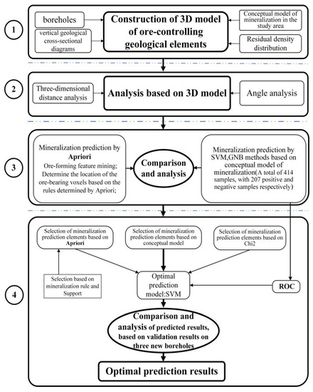
Figure 1.
Technology roadmap for this paper.
As shown in Figure 1, the research process is divided into four steps. The first step (①) involves the construction of a multi-source spatial database of the study area based on the previous knowledge of the study area and related data collected. The database construction is followed by the construction of a solid model of the 3D ore-controlling elements, dividing the study area into regular 3D voxels (25 m × 25 m × 25 m in the X (east–west), Y (south–north), and Z (depth) directions, and in the following text, meter is abbreviated as m). The center point of each 3D voxel carries multi-source attribute data (19 attribute fields). In the second step (②), on the basis of the first step, distance and angle analyses in space are used to provide input data for mineralization prediction in the different models. The points used for distance and orientation analyses with the center point of the 3D voxels originate from the point on the ore-controlling elements that is nearest to the voxels. The third step (③) involves two aspects. (1) The Apriori model is used to mine the ore-forming characteristics of 207 ore-bearing points in drill holes to determine the favorable ore-bearing voxels and the degree of ore-bearing richness based on the rules determined by Apriori. Among them, the distribution of 207 ore-bearing points in 11 known boreholes is shown in Figure 2. (2) In contrast, the mineralization prediction elements are obtained based on the conceptual model of mineralization, the obtained mineralization prediction elements are used as input to the GNB and SVM models, and the two prediction results were compared with the ore-bearing voxels locations determined by Apriori. There are 414 positive and negative samples, of which 207 positive samples are recognized from known drilling data (the 207 positive samples are the same as the data used for Apriori mining), and the negative samples are chosen from ore-free voxels identified in the drill holes and known ore-free places on the surface [29,30]. The fourth step (④) is divided into two aspects: in the first aspect, the optimal prediction model between the SVM and GNB models is determined based on the receiver operating characteristic (ROC) [31]. Then, Apriori and Chi-square are used to filter out the respective mineralization prediction elements. The Chi-square test measures the dependence between random variables, so using this function eliminates the features that are most likely to be independent of the classes and thus irrelevant to the classification [32,33]. In the second aspect, the two sets of screened mineralization prediction elements are predicted using the SVM model, and we compare the two kinds of prediction results with the original mineralization prediction elements derived from the mineralization conceptual model. The four steps are used to complete the comparison in different dimensions and levels and to analyze the characteristics of each of the models and the differences in their prediction results.
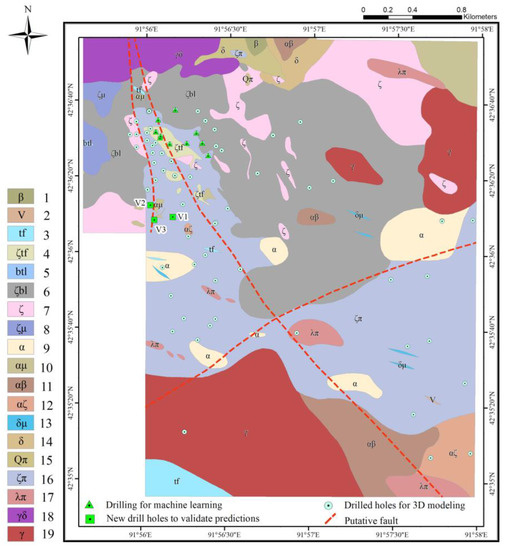
Figure 2.
Comprehensive geological maps of Meiling South. 1 basalt, 2 gabbro, 3 tuff, 4 dacite tuff, 5 breccia-bearing tuff lava, 6 anglian breccia lava, 7 dacite, 8 dacite porphyrite, 9 andesite, 10 andesitic porphyrite, 11 andesitic dacite, 12 andesitic dacite, 13 dioritic porphyrite, 14 diorite vein, 15 quartz porphyry, 16 dacite porphyry, 17 rhyolite porphyry, 18 granodiorite, 19 granite dike.
The main findings follow. (1) The Apriori method is used to mine the known ore body property data to derive the spatial distribution characteristics of high and low-grade ore bodies. (2) Apriori has some reference values for MPM and the selection of mineralization prediction elements.
2. Geological Overview of the Study Area
The study area is located in the Meiling South mining area in the Hami region of Xinjiang, China. The area has considerable potential in the development of mineral resources at depth and includes copper–zinc deposits mainly of the volcanogenic massive sulfide (VMS), porphyry, and shallow-forming low-temperature types [34,35]. The comprehensive geological map of the Meiling South study area is shown in Figure 2. The southern part of the area consists mainly of granite veins, andesitic basalt, andesitic, rhyolite porphyry, and tuff. The central area consists mainly of andesitic porphyry and rhyolite porphyry. The northern part mainly comprises andesitic breccia lava, andesite, and granodiorite. Varying degrees of medium acidic rock bodies are distributed throughout. Significant ore-controlling faults in the study area are the northwest and northeast-oriented faults.
2.1. Stratigraphy
The stratigraphy of the study area consists of volcanic rocks of the Daliugou Formation of the Late Ordovician-Early Silurian Arakanpo Group. These marine volcanic rocks and volcanic clastic rocks of active terrestrial nature can be divided into four lithological sections, from bottom to top. The first section is mainly composed of fractured gray and black–gray basalt and andesite basalt with small amounts of basaltic andesite, andesite, and volcanic clastic rocks of the same composition. In the second section, the lower part is composed of blue–gray and greenish–gray andesite, andesitic tuff, fused tuff, and sunken tuff, and the upper part contains blue–gray and greenish–gray andesite, andesitic tuff, sunken tuff, and sand conglomerate. The third section contains black–gray andesitic basalt, andesitic basalt, andesitic fused tuff, tuff, and tuff conglomerate, and often grayish–brown andesitic and andesitic rocks. The fourth section contains grayish–white and light red–gray rhyolite, rhyolitic porphyry, conglomerate-bearing rhyolitic sunken tuff, and brecciated tuffaceous lava. The second and fourth lithologic sections and a small number of third lithologic sections are mainly exposed in the study area. The first lithologic section is not exposed at the surface.
2.2. Igneous Rock
The Middle Ordovician strata are mainly composed of volcanic rocks. A wide range of medium-acid magmatic rocks intrude into the Silurian strata. The main intrusive rock assemblages are Silurian eclogite-granodiorite with small amounts of gabbro and medium acidic, basal shallow-formed rocks. The volcanic magmatic activity in the study area is strong, with a very large set of sodium-rich basal-neutral-acidic volcanic rocks. The rock assemblages are basaltic, andesitic, and rhyolitic with the most developed being medium-acidic volcanic rocks.
2.3. Fault Structure
The study area is well developed in terms of fault structures. In terms of direction, they can be divided into northwest and northeast faults. These include two sets of conjugate faults (north–northeast and north–northwest). A copper–zinc polymetallic mine is located in the volcanic tectonic depression controlled by early tectonics.
Based on the known ore-controlling elements in the study area, a conceptual model for the mineralization of VMS-type copper deposits in the Meiling South area was constructed (Table 1). Next, after combining the available information in the study area, the individual ore-controlling elements of the mineralization prediction model in the study area were determined (Table 2).

Table 1.
Meiling South VMS conceptual model of copper deposit mineralization.
Table 2.
Ore-controlling elements in the mineralization prediction model.
3. Data and Methods
A total of 54 drill holes were collected (Figure 2), of which 51 drill holes were used for 3D geological model construction. The remaining three drill holes were subsequently collected to verify the prediction effect of different mineralization prediction elements.
The research area is divided into 690,120 voxels, and each voxel has 19 attribute fields. These attribute fields express the 3D distance and orientation information to the ore-controlling elements as well as physical property information.
3.1. Data Integration and Pre-Processing
3.1.1. Data Integration and 3D Geological Model Construction
The SKUA-GOCAD software platform was used to explicitly generate the 3D geological model of the study area. The 3D modeling method is the explicit modeling method. The data used included the drill hole data and vertical geological cross-sectional diagrams, which in turn included drill hole data containing information on lithology and its spatial distribution pattern and partly contained copper content information. The lithologies of the drill holes in the study area were categorized and combined to form five main lithologies (Table 3) in order to summarize the characteristics of the mineralization pattern in the study area, avoid confusion between names, and facilitate the construction of a 3D model of the ore-controlling elements in the study area. These lithologies were then combined with the lithologies in the drill holes, residual density data, and vertical geological cross-sectional diagrams formed by expert recognition. The 3D geological solid model of the ore-controlling elements in the study area was constructed, as shown in Figure 3. Figure 3a shows the tuff model, Figure 3b shows the pyritic sericitization model, Figure 3c shows the andesite model, Figure 3d shows the meso-acidic intrusive rock model, Figure 3e shows the lava model, and Figure 3f shows the main fault distribution model.
Table 3.
Categorization of lithologies.
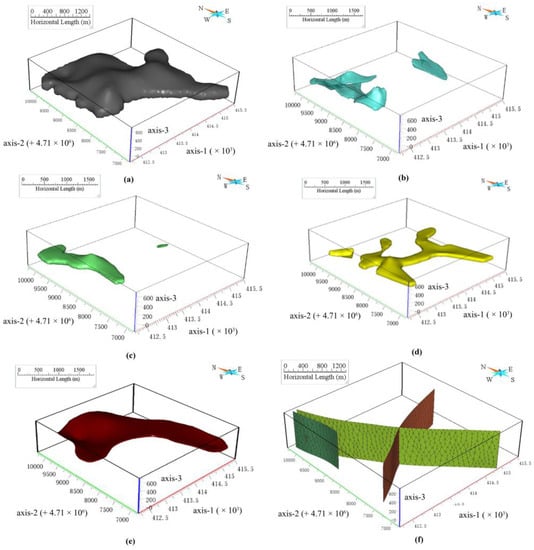
Figure 3.
Three-dimensional (3D) model construction of ore-controlling elements in the study area. (a) Tuff model; (b) Pyrite sericitization model; (c) Andesite model; (d) Meso-acidic intrusive rock model; (e) Lava model; (f) Fault distribution model (Different colors represent different directions of fault).
Next, for the 1:50,000 gravity observations of the study area, the Bouguer gravity anomaly was solved, filtered, and then smoothed to strip the regional anomaly. Then, based on Gra3D, the gravity inversion module of the University of British Columbia (UBC-GIF; Vancouver, BC, Canada), the 3D residual density data below the surface of the study area were obtained, and a horizontal slice map was created (Figure 4). The parameters involved in the inversion process included the GCV inversion mode and depth weighting function. (Generalized cross-validation (GCV) is an inversion model: the GCV model is appropriate for a suitable data grid, but the degree of uncertainty cannot be determined; it employs a computational strategy to seek trade-off parameters to derive the uncertainty of the estimated value). The initial model is set to the 0-value model, the reference model is the default model, and 2.6 g/cm3 is the background field.
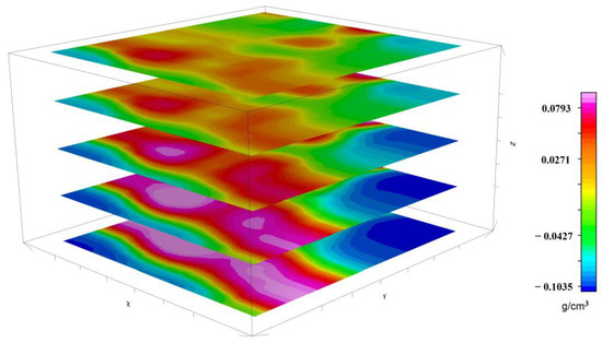
Figure 4.
Residual density distribution data for the study area.
3.1.2. Data Pre-Processing and Coding
The 3D model is expressed as a regular voxel, surface, and solid model. The dimensions of the regular voxels are 25 m × 25 m × 25 m, the total number of voxels in the study area is 690,120, the depth range is 700 m above sea level to 175 m below sea level (0 m for sea level), the span interval is 875 m, and the center point of each voxel is the storage carrier of properties. Using 3D distance and angle analyses, the 3D distance, horizontal angle, and vertical angle of all the voxels from the nearest point of the 3D distance on tuffs, pyritic sericitization, andesites, meso-acidic intrusive rock, and lavas are calculated. The horizontal angle (Figure 5a) ranges from 180° to −180° (0° for east, 90° for north, 180° or −180° for west, and −90° for south; the vertical angle (Figure 5b) is 0° in the horizontal direction, 90° vertically upward, and −90° vertically downward). Both the distance and angle are constituted by the center of the voxels as the origin radiating in the direction of the neighboring points; details can be seen in Figure 5c.
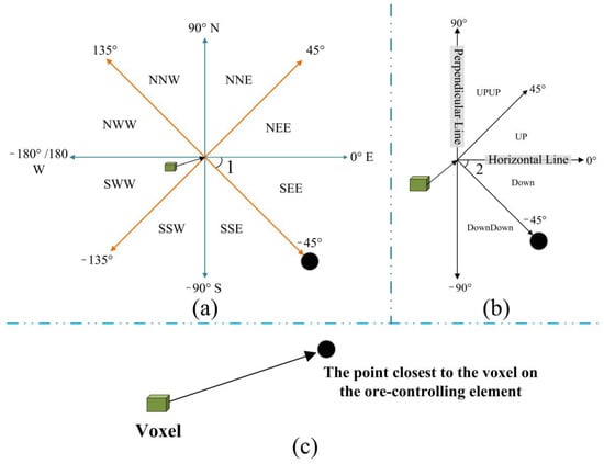
Figure 5.
Schematic diagram of horizontal and vertical angle of voxel distance ore-controlling elements. (a) Schematic diagram of horizontal angle, ∠1; (b) Schematic diagram of vertical angle, ∠2; (c) Schematic diagram of radiating to ore-controlling element points with the voxel as the center. Note: The horizontal angle is the angle between two lines, one of which is the projection of the line connecting the center point of the voxel and the ore-controlling element point on the horizontal plane, and the other line is the 0-degree direction line, as shown in (a); north is positive and south is negative. The vertical angle (b) is the angle formed by the line connecting the voxel center point and the ore-controlling element point and the projection line of this line on the horizontal plane; it is positive for upward and negative for downward.
To meet the subsequent Apriori’s analysis, the original data are respectively coded by category: first, the name of the ore-controlling elements is coded (the code is provided in Table 4). Next, spatial analysis is performed to calculate the 3D distance, horizontal angle, and vertical angle of all the voxels from the ore-controlling elements. The nearest point of the ore-controlling element from the voxel is selected as the calculation point of the distance and angle. For example, after analyzing the pyrite sericitization of the ore-controlling element, we can determine the information of the attribute of the 3D distance of all voxels from the pyrite sericitization, the horizontal angle of all voxels from the pyrite sericitization, and the vertical angle of all voxels from the pyrite sericitization. With the exception of the residual density, the 18-attribute information can be generated for each voxel and each ore-controlling elements (including tuff, pyritic sericitic alteration, andesite, meso-acidic intrusive rocks, lava, and fault). Then, together with the residual density element, we finally determine each voxel in the 3D space with 19 pieces of attribute information, and we encode each attribute separately (Table 5). To explain the information in the table as an example of the ore-controlling elements, we use pyritic sericitic alteration, where the pyritic sericitic alteration code is 3, and the voxel is coded as J33D from the pyritic sericitic alteration 3D distance. The distance from the pyritic sericitic alteration 3D distance is sub-coded as 330, 360, 390, and 3120, respectively, indicating that 330 means 0 m < J33D ≤ 30 m, 360 means 30 m < J33D ≤ 60 m, 390 means 60 m < J33D ≤ 90 m, and 3120 means 90 m < J33D ≤120 m. Ore-controlling elements with 3D distances greater than 120 m from the voxel are excluded from the voxel’s attributes to ensure that the attribute information with a closer relationship to the ore-bearing points is mined. The horizontal angle of the voxel from the pyritic sericitic alteration is coded as J3H. The horizontal angle of the voxel from the pyritic sericitic alteration is sub-coded as 3NNE, 3NEE, 3SEE, 3SSE, 3SSW, 3SWW, 3NWW, and 3NNW, where 3NNE means 45° < J3H < 90° (Figure 5a). The vertical angle of the voxel from the pyritic sericitic alteration is coded as J3V, and all voxels from the pyritic sericitic alteration vertical angle sub-codes are 3UU, 3U, 3D, and 3DD. The vertical angle of 3DD represents the vertical angle from the pyritic sericitic alteration as DownDown in Figure 5b, which is located between −90° and −45°, i.e., −90° ≤ J3V < −45°, where 3UU represents 45° < J3V ≤ 90° and so on, U represents Up, and D represents Down.
Table 4.
Level 1 codes for ore-controlling elements.
Table 5.
Multi-level coding table for ore-controlling elements.
In addition, the 3D voxel containing ores are classified into four classes according to their copper element content, i.e., 41, 42, 43 and 44, where 41 represents the copper element content between 0.0 and 0.01%, 44 represents the copper element content between 0.18% and 4.04%, 42 means 0.01% < copper element content ≤ 0.05%, and 43 means 0.05% < copper element content ≤ 0.18%. This classification is based on a natural interruption point grading according to the copper element content. The residual density is divided into 5 levels according to the natural interruption point: 1 means −0.106 < residual density ≤ −0.056, 2 means −0.056 < residual density ≤ −0.019, 3 means −0.019 < residual density ≤ 0.01, 4 means 0.01 < residual density ≤ 0.04, 5 means 0.04 < residual density ≤ 0.09, and the unit of value is g/cm3.
Finally, the points used for Apriori mining are the 207 ore-bearing points in the borehole, and the 19 attributes contained in all the voxels are used to determine the location of the ore-bearing voxels according to the rules of Apriori mining.
3.2. Principles of the Method
In this paper, a comparative study of mineralization information mining and deep prediction was performed based on the Apriori algorithm and SVM and GNB models. Based on the R language, the R version is version 3.5.3, and the Apriori algorithm is completed using the open source packages arules and arulesViz. GNB and SVM were applied utilizing the open-source toolkit scikit-learn 0.23.2 based on Python. The principles and parameters of the three algorithms are detailed in Section 3.2.1, Section 3.2.2 and Section 3.2.3.
3.2.1. Apriori Model
The Apriori algorithm is used to mine the data association rules [36]. The smallest unit is the item set. In this paper, the item set is each attribute of each voxel in the 3D space. The combination of different items appearing in the item sets constitutes the association rules. The rules are mined and, based on this, their potential laws are analyzed.
Two basic concepts are involved in the basic definition of the Apriori algorithm.
In the first concept, a threshold is set for the minimum support. If the support of an item set is greater than or equal to the minimum support threshold, it is a frequent item set. If the support of an item set is less than the minimum support threshold, it is an infrequent item set. In the second concept, if an item set is a frequent set, then all of its subsets are frequent sets. If it is an infrequent set, then all of its parents are infrequent sets. This is because all subsets of an item set have support greater than or equal to itself, while all parents of an item set have support less than or equal to itself.
The Apriori algorithm uses an iterative approach. In this approach, the first search is for candidate item sets and their corresponding support thresholds. This is followed by pruning to remove the item sets with values below the support threshold to obtain the frequent item sets. The remaining frequent item sets are concatenated to obtain the candidate frequent item sets. These sets are filtered to remove the candidate frequent item sets with values below the support threshold to obtain the true frequent item sets, and so on. This is iteratively performed until the frequent k + 1 item sets cannot be found. The set of corresponding frequent k item sets is the output of the algorithm [37].
Three commonly used metrics for the evaluation of frequent item sets are support, confidence, and lift. Support is the number of times several associated data items appear in the item sets as a proportion of the total item sets. Or the probability of the occurrence of several data associations. Support (X) is calculated as (Formula (1)):
Illustrate: X denotes one item set and M denotes the sum of all item sets.
The confidence level reflects the probability that one item set will occur after another or the conditional probability of the item set. The confidence level of X on Y is calculated as Formula (2):
Illustrate: Support (X⋃Y) indicates the probability that X and Y occur at the same time.
Lift denotes the ratio of the probability of containing X at the same time, which is conditional on containing Y, to the probability of X occurring alone. Lift reflects the association between X and Y. If the lift is greater than 1,X− > Y, then it is a valid strong association rule. If lift is less than or equal to 1, X− > Y, then it is an invalid strong association rule. A special case is that if X and Y are independent, then lift (X− > Y) = 1, since at this point, P (X/Y) = P (X). In short, the lift is the number of times there is a likelihood of finding the set of items Y in the set of items for which X exists compared to finding the set of items Y from the set of all items; see Formula (3).
For application in this article, the minimum support was set to 0.1, the minimum confidence level was set to 0.5, the lift value was greater than 2, and the minimum number of items was set to 5. The setting of minimum support, minimum confidence, and lift indicators is determined by repeatedly testing different values and comparing the resulting rules. Then, by setting the Right-Hand Side (RHS) as 44 (ore-bearing points with a relatively high copper element content, 0.18% < copper element content ≤ 4.04%) and 41 (ore-bearing points with a relatively low copper elemental content, 0.0 < copper element content ≤ 0.01%), the rules favoring the formation of relatively high- and low-grade ore bodies were assessed by Apriori mining. RHS is the right part of a rule, and LHS (Left-Hand Side) is the left part of the rule. The rule was not formed after setting 42 and 43 as RHS under the previous support, confidence, and lift indicators settings. This is related to the fact that 42 and 43 are not frequent item sets; therefore, 42 and 43 are not mentioned in the next section.
3.2.2. GNB Model
GNB consists of a set of supervised learning algorithms based on Bayes’ theorem, assuming that the features are independent of one another [38]. For the category labels and to , the associated feature vector, termed Bayes’ theorem, states the following relationship, as shown in Formula (4):
indicates the probability of occurring when occur;
refers to the probability of occurrence of ;
refers to the probability of occurrence of ;
indicates the probability of occurring when occurs;
GNB applies a Gaussian Naive Bayesian algorithm to the classification [39]. The probability of the features is assumed to be Gaussian distributed.
In this paper, the Gaussian Naive Bayesian method was selected, because Bayesian methods are representative of traditional statistical methods. For example, the weight of evidence and other methods are all extensions of Bayesian methods, although in the field of geology, it is difficult to ensure the independence between the various layers of evidence, which can lead to a large prediction probability. For this reason, the prediction results of the GNB method can be used as a broader prediction result in comparative analyses with the results of other prediction methods.
3.2.3. SVM Model
The SVM classification method involves finding a hyperplane in the data distribution as a decision boundary [40] to make the classification error of the model on the data as small as possible, particularly the classification error on unknown datasets [41]. In geometry, a hyperplane is a subspace of a space that is one dimension smaller than the space in which it is located. If the data space itself is 3D, then its hyperplane is a 2D plane. In a binary classification problem, a hyperplane is capable of dividing the data into two sets, each of which contains a separate class. An SVM is a classifier that classifies data by locating the decision boundary with the largest margins [42].
Kernel function is the key to SVM. By mapping the original input space to a higher-dimensional feature space, the originally linearly indistinguishable samples can become linearly distinguishable in the new kernel space [43]. Common kernels include the polynomial kernel function, radial basis function (RBF), see Formula (5), and sigmoid.
Illustrate: where is specified by the parameter gamma and must be greater than 0; are samples.
The SVM prediction model was trained on 80% of the training samples, using a grid search to determine the optimal penalty parameter C. The search interval of this parameter was 0.01 to 7. Equal steps were used to form 70 data. A grid search was conducted using StratifiedShuffleSplit cross-validation. The data were divided into 25 sub-datasets. The test set accounted for 0.3. The SVM kernel function was rbf, and gamma was set to “scale”. The optimal penalty parameter C determined by the grid search was 6.1895.
In this paper, RBF was chosen as the kernel function for SVM.
4. Results and Discussion
4.1. Analysis of Distance and Angle in 3D Space
The 3D distance and angle analyses revealed two properties for the spatial points (or voxels). One is its own residual density, which expresses its own physical characteristics. The other property is the respective 3D distances, horizontal angles, and vertical angles between each point and ore-controlling elements. First, the information on the 19 individual attributes of the 207 ore-bearing points was counted, see Table 6, with column J33D as an example; the mean value of the 3D distance of the point from the pyritic serpentinization is 48.52 m, the standard deviation is 27.67 m, the minimum value is 7.81 m, and the value at 25%, 50%, and 75% of the distribution is 31.49 m, 37.58 m, and 76.23 m, respectively. The relationship between the ore-bearing points and ore-controlling elements can be understood, which in turn refines the understanding of the mineralization law. For example, the 3D distance (J33D) of the ore-bearing points from the pyritic sericite mineralization ranges from 7.81 m to 103.87 m, the horizontal angle is between −152.51° and 169.12°, and the vertical angle is between −66.89° and 75.35°. This reflects the close proximity of the known ore-bearing points to the pyritic sericite mineralization. Half of the ore-bearing points are located in the upper part of the pyrite sericitization mineralization, and the vertical angle is −36.72°. The horizontal angle (JFH) between the known ore-bearing points and the fault is between −164.75° and 41.55°. This reflects the fact that the south and northeast–east of the ore-bearing point are faults.
Table 6.
Statistics of 19 attributes of known ore-bearing points.
The same statistical analysis was also performed for the 690,120 individual voxels within the study area (Table 7). Figure 6(a1, a2, a3, a4, a5, and a6), respectively, indicate the 3D spatial distance of each voxel from tuffs, pyritic sericitization, andesites, meso-acidic intrusive rock, lava, and fault. Figure 6(b1, b2, b3, b4, b5, and b6), respectively, indicate the horizontal angle of each voxel from tuffs, pyritic sericitization, andesites, meso-acidic intrusive rock, lava, and fault. Figure 6(c1, c2, c3, c4, c5, and c6), respectively, indicate the vertical angle of each voxel from tuffs, pyritic sericitization, andesites, meso-acidic intrusive rock, lava, and fault.
Table 7.
Statistics of 19 attributes of all voxels.
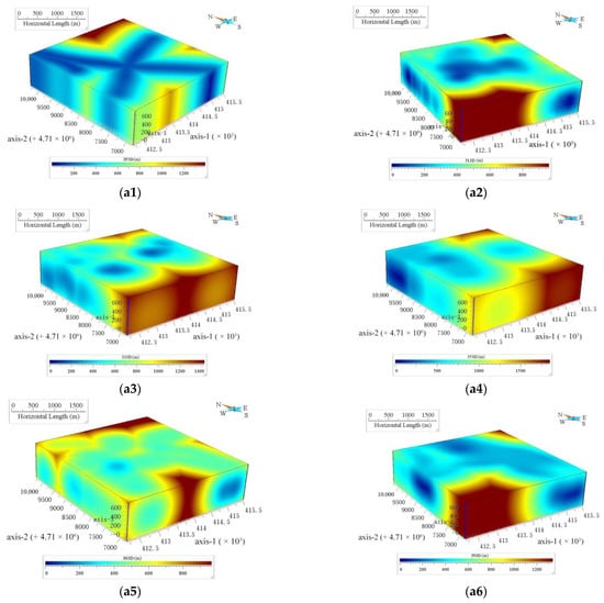
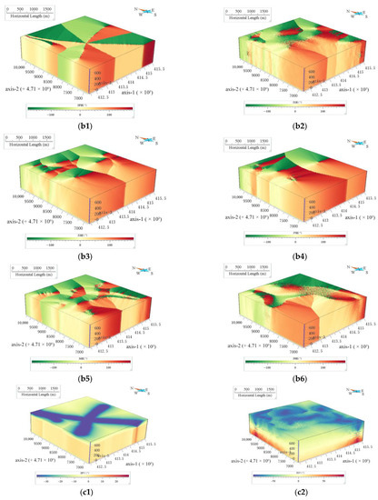
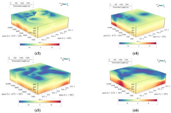
Figure 6.
(a1) Three-dimensional (3D) distance from voxel to the fault; (a2) 3D distance from voxel to the tuff; (a3) 3D distance from voxel to the pyritic sericitization; (a4) 3D distance from voxel to the andesite; (a5) 3D distance from voxel to the meso-acidic intrusive rock; (a6) 3D distance from voxel to the lava. (b1) Horizontal angle from voxel to the fault; (b2) Horizontal angle from voxel to the tuff; (b3) Horizontal angle from voxel to the pyritic sericitization; (b4) Horizontal angle from voxel to the andesite; (b5) Horizontal angle from voxel to the meso-acidic intrusive rock; (b6) Horizontal angle from voxel to the lava. Three-dimensional (3D) distance and orientation information from voxel to the ore-controlling elements. (c1) Vertical angle from voxel to the fault; (c2) Vertical angle from voxel to the tuff; (c3) Vertical angle from voxel to the pyritic sericitization; (c4) Vertical angle from voxel to the andesite; (c5) Vertical angle from voxel to the meso-acidic intrusive rock; (c6) Vertical angle from voxel to the lava.
4.2. Apriori Algorithm-Based Association Rule Mining and Favorable Voxel
The mining attribute information of 207 ore-bearing points is based on Apriori. First, as shown in Figure 7a, the results are based on the order of support from largest to smallest and listing the top 10. The properties of 9UU, 530, and other attributes were frequently and strongly correlated with the ore-bearing points. The contribution to the mineralization of the point was also evident. The top three were the remaining density of the ore-bearing points > −0.056 g/cm3 and ≤−0.019 g/cm3, the vertical angle of the point from the lava between 45° and 90°, and the 3D distance of the point from the andesite between 0 and 30 m.
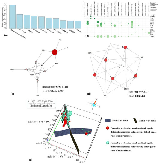
Figure 7.
Series of graphs generated based on Apriori. (a) Top 10 single item sets with support; (b) Rules for when the lift is greater than 2 and the LHS and RHS item sets contain both low-grade (41) and high-grade ores (44); (c) Top 5 rules for low-grade ore; (d) Top 5 rules for high-grade ore; (e) Favorable ore-bearing voxels and their spatial distribution screened out according to low-grade and high-grade rules of mineralization.
Second, after further filtering of the 24,859 rules generated by Apriori, there were a total of 768 rules in Figure 7b, among which 209 rules were for forming low-grade ore, and seven rules were for the formation of high-grade ore. Those whose lift value exceeded two and whose LHS and RHS sets contained a single item set 41 (low-grade ore) or 44 (high-grade ore) were further extracted to form the graph shown in Figure 7c. In this graph, the LHS is the horizontal axis, and the RHS is the vertical axis. Taking one of the rules as an example, {130,360,530, FNEE} => {44}, {130,360,530, FNEE} is the LHS, and {44} is the RHS. These rules indicate that the presence of LHS plays a certain role in promoting RHS and that the role depends on the size of the lift value, while the former rules for the formation of low-grade and high-grade ore are taken separately to form a rule-pointing diagram, as shown in Figure 7c,d, in which the right item set RHS is the final pointing position of the arrow, and the left item set LHS is the starting point of the arrow and points to the circle. The size of the circle is determined by the support value; the larger the support value, the larger the circle. In addition, a darker color indicates a larger lift value, and vice versa.
Third, a comprehensive judgment of the rules for the formation of low-grade ore (Figure 7c), combined with support, confidence, and lift values, revealed the voxels to the fault forming the southeast–east azimuth, −45° < JFH ≤ 0°, and the voxels to the lava forming the southeast–east azimuth, −45° < J9H ≤ 0°. The voxels are located below the tuff and above the pyritic sericitization. Voxels are 60 m from tuff and 30 m from andesite. Furthermore, for the voxel within a range of 30 m from the fault, the remaining density distribution was between −0.056 and −0.019 g/cm3. The coexistence of the above- mentioned elements facilitated the formation of an ore-bearing voxel containing relatively low-grade ore bodies.
Fourth, comprehensive judgment of the rules for the formation of high-grade ore (Figure 7d), combined with support, confidence, and lift values, revealed the location of the voxels northeast–east from the fault between 0 and 45°, the voxels within a 3D spatial distance of 30 m from andesite and tuff, and voxels within a 3D spatial distance of 60 m from Pyritic sericite alteration. Furthermore, the remaining density distribution between −0.056 and −0.019 g/cm3 performs the function of enrichment to form higher-grade ore bodies; it is speculated that this is related to multi-stage mineralization and fault properties.
Fifth, combined with professional knowledge to judge the extracted rules and integrate the indicators, the voxels with the above rules (i.e., attribute) in the 3D space of the study area were screened, and their spatial distribution was visualized centrally; see Figure 7e. Comparison of the points with the known element content of copper revealed that the mineralization rules forming high- and low-grade ore overlapped well with the spatial location of known ore-bearing points, completely covering the known ore-bearing points. The other voxels with unknown mineralization are evaluated to determine whether they have the item set in the LHS of the rules (i.e., the property information of the voxels). Combined with professional knowledge, this can be used as the basis to determine whether they are likely to form ore bodies. In addition, the high and low element content corresponds to the rules of forming high-grade ore and low-grade ore, which reflects the effectiveness of the Apriori algorithm for implicit information mining, such as the discovery of the distribution patterns of high and low ore bodies.
4.3. Comparison of Ore-Bearing Voxels Determined by APRIORI with SVM and GNB Prediction Results
The learning databases of GNB and SVM were constructed in the study area. The ratio of positive and negative samples was 1:1, the sum of positive and negative samples was 414 individual points, and the training and test sets were divided in a ratio of 8:2. All attributes of the spatial voxels were normalized, and the value interval was transformed between 0 and 1 to eliminate the influence of different magnitudes on the accuracy of the model. The parameters and prediction results are summarized in Section 4.3.1, Section 4.3.2 and Section 4.3.3. Table 6 provides the attribute information for the 207 positive samples.
4.3.1. GNB Model Prediction Results
Overall, 80% of the sample data were divided for learning to ensure the learning effect of the model in the limited number of samples. Next, the StratifiedShuffleSplit method was used to divide 80% of the training sample data into ten sub-datasets, of which the sub-test set was 30%, and the learning curve of the GNB model was drawn (Figure 8a). With the increased number of training samples, the sub-test set scores of the cross-validation dataset gradually converged with the scores of the training dataset. In addition, the training score finally stabilized at a value > 0.8. The trained model was tested in 20% of the sample data not involved in training. The positive sample prediction accuracy reached 0.83 (Figure 8b). In the ROC curve of GNB on the test set, the area under the ROC curve (AUC) value of GNB was 0.905, according to Figure 9. The trained model was predicted using the whole voxels. The predicted probability cross-section of voxels mineralization in the study area was thus obtained (Figure 8c).
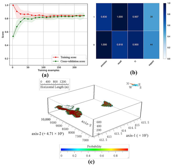
Figure 8.
GNB learning process and its prediction results. (a) The learning curve of the GNB; (b) GNB classification report (the test sample accounts for 0.2 of the total 414 positive and negative samples); (c) Probability cross-section of GNB prediction results.
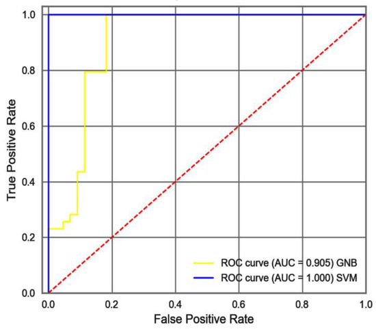
Figure 9.
ROC curve based on the test dataset (the test sample accounts for 0.2 of the total 414 positive and negative samples).
4.3.2. SVM Model Prediction Results
According to Figure 10a, as this parameter reached 6.1895, the accuracy curve of the entire model on the sub-test and sub-training datasets converged to a steady state. The SVM was also plotted in the learning process using the learning curve of hierarchical cross-validation, as shown in Figure 10b. With the increase in training samples, the accuracy of the test set in cross-validation continued to improve and tended to be stable, exceeding 0.9. In addition, we tested the trained model on the test data that account for 20% of the total sample and are not involved in the model training, with positive sample prediction accuracy reaching 1, in Figure 10c. In the ROC curve, the AUC value was 1, as shown in Figure 9. The trained model was predicted on the whole voxels, and the predicted probability cross-section of voxels mineralization in the study area was obtained (Figure 10d).
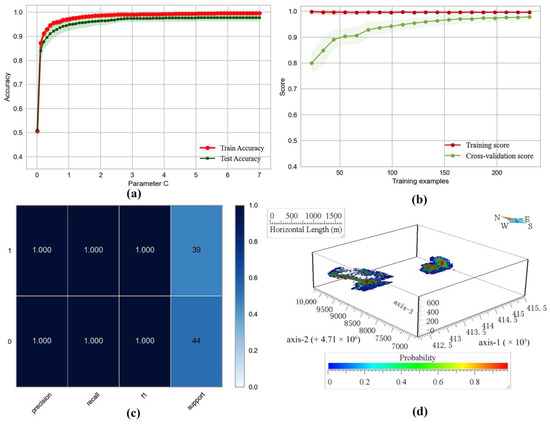
Figure 10.
The result of SVM prediction and its training process. (a) Validation curve for penalty parameter C (parameter C and accuracy); (b) Learning curves (SVM, RBF kernel, C = 6.1895); (c) SVM classification report (the test sample accounts for 0.2 of the total 414 positive and negative samples); (d) Probability cross-section of SVM prediction results.
4.3.3. Analyze the Variability of the Prediction Results of Different Models
Comparison of the mineralization prediction results of the ore-bearing voxels determined by Apriori with those determined by the GNB and SVM models revealed some overlap between the mineralization prediction results in terms of spatial location. According to Figure 11 and Figure 7e, the locations of the ore-bearing voxels determined based on Apriori are more closely related to the ore-controlling elements; they are distributed along the faults distribution and specific lithology according to the mineralization rules, while the locations of the ore-bearing voxels determined by SVM and GNB are more in line with the generalization ability of the mathematical model, widely distributed and representative. Still, in general, the prediction trends of the three methods are the same. Furthermore, among the ore-bearing voxels (1631 voxels) identified by rules of low-grade ore mined by Apriori, the percentages of voxels predicted to be ore-bearing by SVM and GNB were 21.5% and 34.6% (Figure 12), respectively. Among the ore-bearing voxels (1682 voxels) identified by rules of high-grade ore mined by Apriori, the percentage of voxels predicted to be mineral-bearing by SVM and GNB were 45.3% and 54.0% (Figure 12), respectively. The high-grade ore-bearing voxels determined by Apriori are in higher agreement with the mineralization prediction results of the GNB and SVM models, which in turn corroborate each other. To summarize the above, the high and low-grade ore-forming rules identified by Apriori can provide an effective method for further research on the mining of potentially favorable information from multi-source big data.
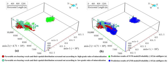
Figure 11.
(a) Comparison of ore-bearing voxels determined by Apriori with SVM prediction results; and (b) Comparison of ore-bearing voxels determined by Apriori with GNB prediction results.
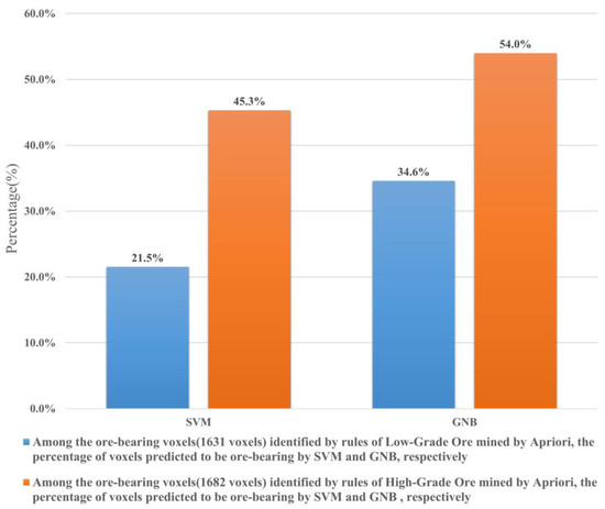
Figure 12.
Among the ore-bearing voxels identified by Apriori, the percentage of voxels predicted to be ore-bearing by GNB and SVM, respectively.
4.4. Comparison of Prediction Results of Different Mineralization Prediction Elements in the SVM Prediction Model
The features selected by Apriori were based on multiple metrics for each item set. The rules to filter out the frequent occurrence of these individual itemsets (i.e., the attributes contained in each voxel; see Table 5) represent the greater importance of the itemsets and the higher-level coding feature. Therefore, based on these considerations, the features shown in Table 8 were determined as the Apriori-identified mineralization prediction elements. For comparison, nine features were also selected by the Chi-square method, as shown in Table 9.
Table 8.
Mineralization prediction elements identified by Apriori.
Table 9.
Mineralization prediction elements identified by Chi2.
Based on the newly selected features of Apriori, the previously selected optimal prediction model (the SVM model) was trained. The grid search used the StratifiedShuffleSplit cross-validation and divided one dataset into 25 subsets; the rest of the settings remain the same as before. The verification curve of the penalty parameter C revealed that when the prediction accuracy of the SVM model gradually became stable, the C value corresponding to the 19 mineralization prediction elements reached 6.1895 (Figure 10a), the C value corresponding to the mineralization prediction elements determined by Chi-square reached 6.8986 (Figure 13b), and for the mineralization prediction elements determined by Apriori, the corresponding C value reached 6.8986 (Figure 13d). According to Figure 13a,c, the SVM model reaches a steady state under different mineralization prediction elements, and in conjunction with Figure 10, the SVM models all achieve good training results relative to the predictive elements identified by the conceptual model in the SVM. The model’s accuracy on the training dataset is higher than on the test set, indicating a mild overfitting problem that affects assessment accuracy. Therefore, it is necessary to validate the V1, V2, and V3 boreholes in Figure 14.
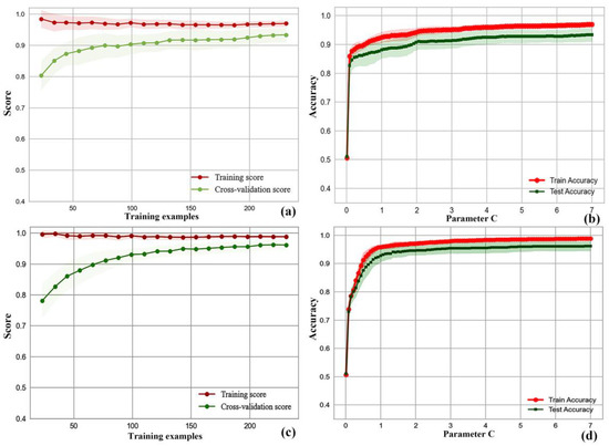
Figure 13.
Training process of different mineralization prediction elements on the SVM model. (a) Learning curve of Chi-square-based mineralization prediction elements on SVM; (b) Parameter C validation curve for Chi-square-based mineralization prediction elements on SVM; (c) Learning curve of Apriori-based mineralization prediction elements on SVM; (d) Parameter C validation curve for Apriori-based mineralization prediction elements on SVM.
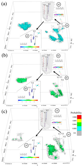
Figure 14.
Prediction results for different mineralization prediction elements on SVM. (a) Equivalence surface distribution of prediction results based on original mineralization prediction elements determined by conceptual model; (b) Equivalent surface distribution of prediction results based on the mineralization prediction elements determined by Chi-square; (c) Equivalent surface distribution of prediction results based on the mineralization prediction elements determined by Apriori, where a1, b1, and c1 are the actual locations of drill holes V1, V2, and V3 in the main view; a2, b2, and c2 are the elemental copper content of the ore bodies in drill holes V1, V2, and V3; a3, b3, and c3 are the probabilities of the voxels surrounding the ore bodies in drill holes V1, V2, and V3; a3 corresponds to the conceptual model of mineralization, b3 to Chi-square, and c3 to Apriori.
Based on the SVM prediction results of the different mineralization prediction elements, validation was carried out with the newly collected drill holes. The locations of the drill holes are shown in Figure 1 (In Figure 1, subplots a2, a3, b2, b3, c2, and c3 are all insets and are not on the same scale as the rest of Figure 1). To make the prediction results concrete and practical with respect to their contribution to validation, the prediction results of probability in the surrounding 30 m of the ore body of drill holes were taken as the validation dataset. The prediction results of the different mineralization prediction elements on these voxels obtained by the SVM model were compared. As shown in Figure 14a–c, Figure 14(a1–c1) shows the locations of the three validation holes V1, V2, and V3 in the predicted probability distribution. Figure 14(a2–c2) shows the location and copper content distribution of the validation drill holes V1, V2, V3, with copper content ranging from 0.01% to 2.67%, including the high-grade copper ore body with 2.77% in drill hole V2. Figure 14(a3–c3) shows the predicted probability distribution of voxels around the ore location. The prediction results through the mineralization prediction elements determined by Apriori have more voxels with prediction probabilities greater than 0.5, which are 6, 5, and 1 in the three drill holes V1, V2, and V3, respectively. From the prediction results, considering the maximum, minimum, and average probabilities (Table 10), Apriori performs better in the selection of mineralization prediction elements when compared to the original 19 mineralization prediction elements and the nine mineralization prediction elements provided by Chi-square.
Table 10.
Predicted results of the validation borehole.
However, the study also has some limitations. The limitations are that the prediction results of different mineralization prediction elements have only been verified in a limited number of drill holes so far. The mineralization prediction elements extracted by different methods have only been tested on one model of SVM, and although the SVM model performs stably throughout, its representativeness is still limited.
5. Conclusions
In this paper, a geological model of the study area was established using drill hole data with the Meiling South mining area in Xinjiang as the study area. The mining of mineralization information was carried out based on the Apriori algorithm, and combined with the SVM algorithm, a comparative study of the prediction of different mineralization prediction elements was carried out, and the following two insights were obtained:
1. Based on the Apriori algorithm, the rules for forming high- and low-grade ore bodies can be mined based on the known attributes of the ore-bearing points: the distribution of high and low-grade ore bodies is closely related to the three-dimensional distance and angle of ore-bearing points to specific ore-controlling elements.
2. The three sets of mineralization prediction elements were formed by the conceptual model of mineralization, Chi-square, and Apriori. We compared their prediction results on the SVM model and verified them on the new drill hole, and the prediction results formed by the mineralization prediction elements determined by Apriori have high accuracy.
The innovation of this paper lies in the introduction of Apriori into 3D MPM and corresponds to the above two conclusions with two specific innovations as follows:
Corresponding to conclusion 1, the innovation of this paper is to classify the copper elemental content of the ore-bearing points with other attributes of the ore-bearing points and to use the Apriori method for correlation analysis. Thereby, effective rules favoring the formation of high-grade and low-grade ore bodies are found among the ore-bearing point attributes. This method quantitatively evaluates the interactions among the ore-bearing point attributes. It is a reference value for the future identification of mineralization rules in 3D space.
Corresponding to conclusion 2, the innovation of this paper also lies in the fact that combining the data mining method (Apriori) to form the elements of mineralization prediction and the machine learning method improves the accuracy of 3D MPM to some extent. This combined approach avoids feeding too much data as the input data set into the SVM for training, thus improving the evaluation results of the SVM. The combined approach used in this paper can be applied to other regions and helps to mine potential information and improve the accuracy of 3D MPM.
Nevertheless, there are limitations to the wide application of the whole methodological system in this paper, such as the comprehensive validation of multiple models, and the accuracy of the prediction results cannot be verified in more new drill holes due to the time and data acquisition factors. In the future, we will continue to conduct more in-depth research on mining 3D mineralization information.
Author Contributions
Writing—original draft preparation, J.C.; the proposer and designer of the research idea, conceptualization, methodology, funding acquisition, project administration, supervision, organized the paper, N.Z.; project administration, supervision, modification suggestion, K.Z.; proofreading, revision, J.T., L.C., H.Z. and Y.C.; All authors have read and agreed to the published version of the manuscript.
Funding
This work was supported by the Major Science and Technology Project of Xinjiang Uygur Autonomous Region (grant number 2021A03001-4); the Young Scholars in Western China, the Chinese Academy of Sciences (grant number 2020-XBQNXZ-014); the Xinjiang Science Foundation for Distinguished Young Scholars (grant number 2022D01E01); the “Tianshan Talents” training program (2022TSYCLJ0010).
Data Availability Statement
The data presented in this study are available on request from the corresponding author. The data are not publicly available due to sensitive data involved.
Conflicts of Interest
The authors declare no conflict of interest.
References
- Huang, J.X.; Liu, Z.K.; Deng, H.; Li, L.J.; Mao, X.C.; Liu, J.X. Exploring Multiscale Non-stationary Influence of Ore-Controlling Factors on Mineralization in 3D Geological Space. Nat. Resour. Res. 2022, 31, 3079–3100. [Google Scholar] [CrossRef]
- Liu, Y.; Carranza, E.J.M.; Xia, Q.L. Developments in Quantitative Assessment and Modeling of Mineral Resource Potential: An Overview. Nat. Resour. Res. 2022, 31, 1825–1840. [Google Scholar] [CrossRef]
- Talebi, H.; Mueller, U.; Peeters, L.J.M.; Otto, A.; de Caritat, P.; Tolosana-Delgado, R.; van den Boogaart, K.G. Stochastic Modelling of Mineral Exploration Targets. Math. Geosci. 2022, 54, 593–621. [Google Scholar] [CrossRef]
- Li, S.; Liu, C.; Chen, J. Mineral Prospecting Prediction via Transfer Learning Based on Geological Big Data: A Case Study of Huayuan, Hunan, China. Minerals 2023, 13, 504. [Google Scholar] [CrossRef]
- Kong, Y.H.; Chen, G.D.; Liu, B.L.; Xie, M.; Yu, Z.B.; Li, C.; Wu, Y.X.; Gao, Y.X.; Zha, S.; Zhang, H.Y.; et al. 3D Mineral Prospectivity Mapping of Zaozigou Gold Deposit, West Qinling, China: Deep Learning-Based Mineral Prediction. Minerals 2022, 12, 1361. [Google Scholar] [CrossRef]
- Chen, J.; Jiang, L.; Peng, C.; Liu, Z.; Deng, H.; Xiao, K.; Mao, X. Quantitative resource assessment of hydrothermal gold deposits based on 3D geological modeling and improved volume method: Application in the Jiaodong gold Province, Eastern China. Ore Geol. Rev. 2022, 153, 105282. [Google Scholar] [CrossRef]
- Huang, J.X.; Mao, X.C.; Chen, J.; Deng, H.; Dick, E.M.; Liu, Z.K. Exploring Spatially Non-stationary Relationships in the Determinants of Mineralization in 3D Geological Space. Nat. Resour. Res. 2020, 29, 439–458. [Google Scholar] [CrossRef]
- Chen, J.; Mao, X.; Liu, Z.; Deng, H. Three-dimensional Metallogenic Prediction Based on Random Forest Classification Algorithm for the Dayingezhuang Gold Deposit. Geotecton. Metallog. 2020, 44, 231–241. [Google Scholar]
- Huang, J.X.; Mao, X.C.; Deng, H.; Liu, Z.K.; Chen, J.; Xiao, K.Y. An Improved GWR Approach for Exploring the Anisotropic Influence of Ore-Controlling Factors on Mineralization in 3D Space. Nat. Resour. Res. 2022, 31, 2181–2196. [Google Scholar] [CrossRef]
- Zhou, Y.Z.; Wang, J.; Zuo, R.G.; Xiao, F.; Shen, W.J.; Wang, S.G. Machine learning, deep learning and Python language in field of geology. Acta Petrol. Sin. 2018, 34, 3173–3178. [Google Scholar]
- Xie, S.Y.; Huang, N.; Deng, J.; Wu, S.L.; Zhan, M.G.; Carranza, E.J.M.; Zhang, Y.P.; Meng, F.X. Quantitative prediction of prospectivity for Pb-Zn deposits in Guangxi (China) by back-propagation neural network and fuzzy weights-of-evidence modelling. Geochem. Explor. Environ. Anal. 2022, 22, 10. [Google Scholar] [CrossRef]
- Narayan, S.; Konka, S.; Chandra, A.; Abdelrahman, K.; Andras, P.; Eldosouky, A.M. Accuracy assessment of various supervised machine learning algorithms in litho-facies classification from seismic data in the Penobscot field, Scotian Basin. Front. Earth Sci. 2023, 11, 14. [Google Scholar] [CrossRef]
- Sun, T.; Chen, F.; Zhong, L.X.; Liu, W.M.; Wang, Y. GIS-based mineral prospectivity mapping using machine learning methods: A case study from Tongling ore district, eastern China. Ore Geol. Rev. 2019, 109, 26–49. [Google Scholar] [CrossRef]
- Jia, F.; Su, Z.; Nian, H.; Yan, Y.; Yang, G.; Yang, J.; Shi, X.; Li, S.; Li, L.; Sun, F.; et al. 3D Quantitative Metallogenic Prediction of Indium-Rich Ore Bodies in the Dulong Sn-Zn Polymetallic Deposit, Yunnan Province, SW China. Minerals 2022, 12, 1591. [Google Scholar] [CrossRef]
- Li, H.; Li, X.H.; Yuan, F.; Jowitt, S.M.; Dou, F.F.; Zhang, M.M.; Li, X.L.; Li, Y.; Lan, X.Y.; Lu, S.M.; et al. Knowledge-driven based three-dimensional prospectivity modeling of Fe-Cu skarn deposits; a case study of the Fanchang volcanic basin, anhui province, Eastern China. Ore Geol. Rev. 2022, 149, 17. [Google Scholar] [CrossRef]
- Deng, H.; Zheng, Y.; Chen, J.; Yu, S.Y.; Xiao, K.Y.; Mao, X.C. Learning 3D mineral prospectivity from 3D geological models using convolutional neural networks: Application to a structure-controlled hydrothermal gold deposit. Comput. Geosci. 2022, 161, 17. [Google Scholar] [CrossRef]
- Qin, Y.Z.; Liu, L.M.; Wu, W.C. Machine Learning-Based 3D Modeling of Mineral Prospectivity Mapping in the Anqing Orefield, Eastern China. Nat. Resour. Res. 2021, 30, 3099–3120. [Google Scholar] [CrossRef]
- Song, M.C.; Li, S.Y.; Zheng, J.F.; Wang, B.; Fan, J.M.; Yang, Z.L.; Wen, G.J.; Liu, H.B.; He, C.Y.; Zhang, L.L.; et al. A 3D Predictive Method for Deep-Seated Gold Deposits in the Northwest Jiaodong Peninsula and Predicted Results of Main Metallogenic Belts. Minerals 2022, 12, 935. [Google Scholar] [CrossRef]
- Xiao, K.Y.; Xiang, J.; Fan, M.J.; Xu, Y. 3D Mineral Prospectivity Mapping Based on Deep Metallogenic Prediction Theory: A Case Study of the Lala Copper Mine, Sichuan, China. J. Earth Sci. 2021, 32, 348–357. [Google Scholar] [CrossRef]
- Fu, G.M.; Lu, Q.T.; Yan, J.Y.; Farquharson, C.G.; Qi, G.; Zhang, K.; Zhang, Y.Q.; Wang, H.; Luo, F. 3D mineral prospectivity modeling based on machine learning: A case study of the Zhuxi tungsten deposit in northeastern Jiangxi Province, South China. Ore Geol. Rev. 2021, 131, 19. [Google Scholar] [CrossRef]
- Zhang, Z.Q.; Zhang, J.J.; Wang, G.W.; Carranza, E.J.M.; Pang, Z.; Wang, H. From 2D to 3D Modeling of Mineral Prospectivity Using Multi-source Geoscience Datasets, Wulong Gold District, China. Nat. Resour. Res. 2020, 29, 345–364. [Google Scholar] [CrossRef]
- Zhang, M.M.; Zhou, G.Y.; Shen, L.; Zhao, W.G.; Liao, B.S.; Yuan, F.; Li, X.H.; Hu, X.Y.; Wang, C.B. Comparison of 3D prospectivity modeling methods for Fe-Cu skarn deposits: A case study of the Zhuchong Fe-Cu deposit in the Yueshan orefield (Anhui), eastern China. Ore Geol. Rev. 2019, 114, 10. [Google Scholar] [CrossRef]
- Zhang, N.N.; Zhou, K.; Li, D. Back-propagation neural network and support vector machines for gold mineral prospectivity mapping in the Hatu region, Xinjiang, China. Earth Sci. Inform. 2018, 11, 553–566. [Google Scholar] [CrossRef]
- Zhang, Q.P.; Chen, J.P.; Xu, H.; Jia, Y.L.; Chen, X.W.; Jia, Z.; Liu, H. Three-Dimensional Mineral Prospectivity Mapping by XGBoost Modeling: A Case Study of the Lannigou Gold Deposit, China. Nat. Resour. Res. 2022, 31, 1135–1156. [Google Scholar] [CrossRef]
- Liu, L.; Cao, W.; Liu, H.; Ord, A.; Qin, Y.; Zhou, F.; Bi, C. Applying benefits and avoiding pitfalls of 3D computational modeling-based machine learning prediction for exploration targeting: Lessons from two mines in the Tongling-Anqing district, eastern China. Ore Geol. Rev. 2022, 142, 104712. [Google Scholar] [CrossRef]
- He, X.H.; Deng, X.H.; Pirajno, F.; Zhang, J.; Li, C.; Chen, S.B.; Sun, H.W. The genesis of the granitic rocks associated with the Mo-mineralization at the Hongling deposit, eastern Tianshan, NW China: Constraints from geology, geochronology, geochemistry, and Sr-Nd-Hf isotopes. Ore Geol. Rev. 2022, 146, 17. [Google Scholar] [CrossRef]
- Li, D.; Wang, S.; Li, D.; Wang, X. Theories and Technologies of Spatial Data Mining and Knowledge Discovery. Geomat. Inf. Sci. Wuhan Univ. 2002, 27, 221–233. [Google Scholar]
- Wu, X.D.; Kumar, V.; Quinlan, J.R.; Ghosh, J.; Yang, Q.; Motoda, H.; McLachlan, G.J.; Ng, A.; Liu, B.; Yu, P.S.; et al. Top 10 algorithms in data mining. Knowl. Inf. Syst. 2008, 14, 1–37. [Google Scholar] [CrossRef]
- Tao, J.T.; Yuan, F.; Zhang, N.N.; Chang, J.Y. Three-Dimensional Prospectivity Modeling of Honghai Volcanogenic Massive Sulfide Cu-Zn Deposit, Eastern Tianshan, Northwestern China Using Weights of Evidence and Fuzzy Logic. Math. Geosci. 2021, 53, 131–162. [Google Scholar] [CrossRef]
- Tao, J.T.; Zhang, N.N.; Chang, J.Y.; Chen, L.; Zhang, H.; Chi, Y.J. Unlabeled Sample Selection for Mineral Prospectivity Mapping by Semi-supervised Support Vector Machine. Nat. Resour. Res. 2022, 31, 2247–2269. [Google Scholar] [CrossRef]
- Lin, N.; Chen, Y.L.; Liu, H.Q.; Liu, H.L. A Comparative Study of Machine Learning Models with Hyperparameter Optimization Algorithm for Mapping Mineral Prospectivity. Minerals 2021, 11, 159. [Google Scholar] [CrossRef]
- Liu, H.; Setiono, R. Chi2: Feature selection and discretization of numeric attributes. In Proceedings of the 7th International Conference on Tools with Artificial Intelligence (TAI 95), Herndon, VA, USA, 5–8 November 1995; pp. 388–391. [Google Scholar]
- Liu, H.Y.; Zhou, M.C.; Liu, Q. An Embedded Feature Selection Method for Imbalanced Data Classification. IEEE-CAA J. Autom. Sin. 2019, 6, 703–715. [Google Scholar] [CrossRef]
- Mao, Q.G.; Fang, T.H.; Wang, J.B.; Wang, S.L.; Wang, N. Geochronology studies of the Early Paleozoic Honghai massive sulfide deposits and its geological significance in Kalatage area, eastern Tianshan Mountain. Acta Petrol. Sin. 2010, 26, 3017–3026. [Google Scholar]
- Yu, M.J.; Wang, Y.W.; Wang, J.B.; Mao, Q.G.; Deng, X.H.; Sun, Y.; Zhang, R. The mineralization of the Kalatage arc, Eastern Tianshan, NW China: Insights from the geochronology of the Meiling Cu-Zn(-Au) deposit. Ore Geol. Rev. 2019, 107, 72–86. [Google Scholar] [CrossRef]
- Cui, Y.; He, B.; Chen, J.; He, Z.; Liu, Y. Mining metallogenic association rules combining cloud model with apriori algorithm. In Proceedings of the 30th IEEE International Geoscience and Remote Sensing Symposium (IGARSS) on Remote Sensing—Global Vision for Local Action, Honolulu, HI, USA, 25–30 June 2010; pp. 4507–4510. [Google Scholar]
- Bayardo, R.J.; Agrawal, R.; Gunopulos, D. Constraint-based rule mining in large, dense databases. In Proceedings of the 15th International Conference on Date Engineering, Sydney, Australia, 23–26 March 1999; pp. 188–197. [Google Scholar]
- Zhang, H. Exploring conditions for the optimality of Naive bayes. Int. J. Pattern Recognit. Artif. Intell. 2005, 19, 183–198. [Google Scholar] [CrossRef]
- Mizianty, M.; Kurgan, L.; Ogiela, M. Comparative analysis of the impact of discretization on the classification with Naive Bayes and semi-Naive Bayes classifiers. In Proceedings of the 7th International Conference on Machine Learning and Applications, San Diego, CA, USA, 11–13 December 2008; pp. 823–828. [Google Scholar]
- Qi, X.M.; Silvestrov, S.; Nazir, T. Data Classification with Support Vector Machine and Generalized Support Vector Machine. In Proceedings of the 11th International Conference on Mathematical Problems in Engineering, Aerospace and Sciences (ICNPAA), La Rochelle, France, 4–8 July 2016. [Google Scholar]
- Guenther, N.; Schonlau, M. Support vector machines. Stata J. 2016, 16, 917–937. [Google Scholar] [CrossRef]
- Ghezelbash, R.; Maghsoudi, A.; Bigdeli, A.; Carranza, E.J.M. Regional-Scale Mineral Prospectivity Mapping: Support Vector Machines and an Improved Data-Driven Multi-criteria Decision-Making Technique. Nat. Resour. Res. 2021, 30, 1977–2005. [Google Scholar] [CrossRef]
- Burges, C.J.C. A tutorial on Support Vector Machines for pattern recognition. Data Min. Knowl. Discov. 1998, 2, 121–167. [Google Scholar] [CrossRef]
Disclaimer/Publisher’s Note: The statements, opinions and data contained in all publications are solely those of the individual author(s) and contributor(s) and not of MDPI and/or the editor(s). MDPI and/or the editor(s) disclaim responsibility for any injury to people or property resulting from any ideas, methods, instructions or products referred to in the content. |
© 2023 by the authors. Licensee MDPI, Basel, Switzerland. This article is an open access article distributed under the terms and conditions of the Creative Commons Attribution (CC BY) license (https://creativecommons.org/licenses/by/4.0/).