Abstract
When encountering sedimentary rocks with obvious laminations or fracture development zones, the conductivity of the conductive medium in different directions will change significantly, and the subsurface medium will exhibit macroscopic conductivity anisotropy. To analyze the impact of electrical anisotropy on the surface–borehole transient electromagnetic exploration method, we used the finite element method to investigate the electrical anisotropy surface–borehole transient electromagnetic three-dimensional (3D) forward algorithm, in which we used a tetrahedral mesh to spatially discretize the time–domain Maxwell equation. Then, we discretized it using the second-order backward Eulerian difference method, and we obtained the fields through the PARDISO solver. The validity and correctness of the algorithm were verified through comparison of a one-dimensional (1D) anisotropic model, a complex three-dimensional (3D) isotropic model, and a three-dimensional (3D) anisotropic half-space model. A typical anisotropic geological model was constructed to analyze the effects of anisotropic strata and anomalies in the different principal axis directions on the surface–borehole transient electromagnetic response. The results show that the response of the anisotropic medium is related to the direction of the transmitting source, and the response pattern is complex and volatile. The electrical anisotropic anomaly does affect the amplitude, which should be given special attention when performing surface–borehole transient electromagnetic inversion interpretation.
1. Introduction
The transient electromagnetic method (TEM) is a time–domain artificial source electromagnetic method, which has been widely used in coal and mineral exploration and other fields. This method uses an ungrounded loop or grounded line source to emit a pulse signal into the ground, and by observing the secondary field generated by the induction of the subsurface medium [1], the distribution of the electrical characteristics of the strata is detected [2]. The surface–borehole TEM is an electromagnetic exploration method that has been rapidly developed internationally in recent years and has achieved good results in geological prospecting. It has been applied to research on metal ore exploration, tectonic mapping, petroleum, coal, underground water, geothermal energy, permafrost zones, and marine geology [3]. In metal ore exploration, it has mainly been applied to survey blind ore bodies next to or below the boreholes, and it is especially superior when the ore body is too deep and in areas affected by electrical disturbances (such as conductive cover, shallow sulfides, and surface mineralized stratum) [4]. In Canada, Australia, and several other countries, surface–borehole TEM has become a conventional survey method, and many successful examples of deep mineral searches have been reported.
For example: in Canada, a 1280 m deep, 28 m thick rich ore body was identified about 200 m from the drill hole in 1995 in the Falconbridge Lindsley copper and nickel mine area [5,6]. In this method, the transmitting circuit setup is placed on the ground above or near the borehole, bipolar pulses are sent into the underground, and the receiving probe in the borehole measures the transient electromagnetic response generated by the underground geological body induction point-by-point along the borehole [7]. This method has the advantages of low surface electromagnetic or man-made interference and a strong response signal, and it has been widely used in deep ore-prospecting and geological structure retrieval, and it has an especially irreplaceable advantage in metal mining.
Early in-well instruments in vertical wells could only perform resistivity measurements in a single direction, ignoring the influence of the conductivity anisotropy of the formation. With the advances in technology and the emergence of horizontal wells and highly deviated wells, the electrical anisotropy of the formation affects the accuracy of the measurement results, creating many difficulties in the interpretation and evaluation of anisotropic reservoirs [8]. After the phenomenon of electrical anisotropy in sedimentary strata was discovered in 1902, the recursive formula for electromagnetic fields in layered anisotropic media was derived [9]. When the electromagnetic field of electrical source in anisotropic media is studied by numerical simulation [10], the forward modeling problem of one-dimensional (1D) anisotropy has been comprehensively and perfectly elaborated [11]. Subsequently, more geophysicists have made progress in the study of formation anisotropy, conductivity anisotropy, and vector electromagnetic fields [12,13]. In addition, multicomponent and directional induction logging techniques have been proposed and widely studied [14]. For example, the finite element method is used to calculate the geodetic electromagnetic field of a two-dimensional (2D) electrically anisotropic geoelectric section [15], the effect of triaxial anisotropic seabed on TEM response [16], simulation of the frequency domain electromagnetic response in an electrically anisotropic formation applied the finite difference method to a staggered mesh to [17], the electromagnetic response of the logging-while-drilling tool in tilted anisotropic formations is studied by using the vector finite element method [18], the electromagnetic response of a three-dimensional (3D) electrically anomalous body in an anisotropic formation by using the integral equation simulation method [19], the measurement pattern of transient electromagnetism in electrically anisotropic media near the surface [20], the effect of the electrical anisotropy of a one-dimensional (1D) petroleum reservoir on the apparent resistivity in the transient electromagnetic response [21], the forward and inverse of the electrical source transient electromagnetics in a one-dimensional (1D) anisotropic medium are calculated and analyzed [22], the effect of the electrical conductivity anisotropy in different directions on the electromagnetic field components by using the finite volume method [23,24], the forward calculation of the TEM with a loop source and a long offset distance in three-dimensional (3D) anisotropic media by using the finite volume method [25], and the variation characteristics of an axially anisotropic surface–borehole and tunnel–hole transient electromagnetic response with depth are studied by using the finite difference method [26,27]. However, few studies have reported on the TEM in the time domain in anisotropic media surface–borehole logging. Based on the time–domain anisotropic medium response, we used the finite element numerical simulation method to study and analyze the time domain characteristics of the transient electromagnetic response in an anisotropic medium in different directions. The results provide guidance for the interpretation of the anisotropy of the TEM and a reference for anisotropic inversion.
2. Basic Theory
2.1. Control Equations
In isotropic media, resistivity and conductivity are scalar quantities; while, in anisotropic media, resistivity and conductivity can be expressed in tensor form as follows:
For calculation purposes, the arbitrary conductivity tensor can be obtained from the principal axis anisotropy conductivity tensor [28] after three Eulerian rotations, where , , and are referred to as the principal conductivities.
In the Cartesian coordinate system, the x and y-axis lie in the horizontal plane, and the z-axis points vertically upward. First, rotate counterclockwise along the z-axis by angle to obtain the new coordinate system , rotate it counterclockwise along the -axis by an angle of to obtain a new coordinate system , and then rotate counterclockwise along the -axis by an angle of . Finally, the conductivity tensor can be expressed as:
where is the rotation matrix of three counterclockwise rotations.
The angles are the anisotropic strike angle, anisotropic dip angle, and anisotropic declination angle, respectively [29].
The time–domain wave equation satisfied by the electric field intensity vector can be obtained from Maxwell’s set of equations:
where is the magnetic permeability, J is the field source current, is the anisotropic permeability tensor, is the electric field to be sought, and t is the time. The electric field intensity vector satisfies the boundary conditions at the interface of different media:
where is the unit normal vector at the boundary of the medium, and are the electric field intensity vectors in the medium on either side of the boundary.
2.2. Spatial and Time Domain Discretization
By using the finite element method to discretize Equation (7), the residual [13] can be defined according to the Galerkin method:
As in Figure 1, the linear distribution of the electric field within the element is approximated using a non-structural tetrahedral mesh discrete computational region, and the Nédélec vector interpolation basis function that automatically satisfy the tangential components of the electric field are continuous and non-dispersive. In a single finite meshing element , the electric field at an arbitrary position within the element can be expressed as:
where is the electric field to be sought on the prismatic edge of the element, and is the vector difference basis function in the eth element. In practice, the higher-order difference vector basis function can be used to improve the calculation accuracy.
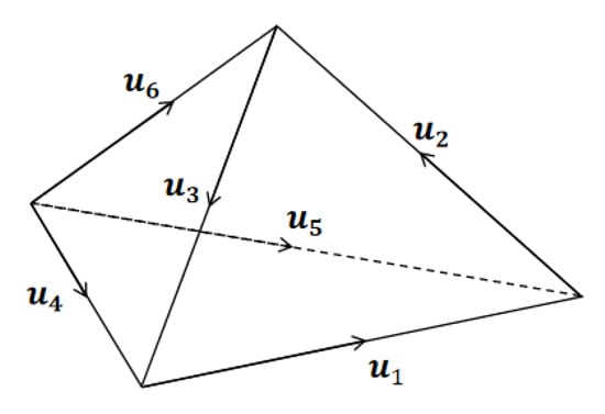
Figure 1.
Free tetrahedral mesh element.
By applying the Galerkin weighted residual method [30], we can obtain:
where is the stiffness matrix, is the mass matrix, and is the source vector. In a single element ,
To improve the numerical accuracy, the time is discretized using a second order backward Eulerian difference format:
where is the time step before the ith hour. Substituting Equation (11) into Equation (15) yields:
The resulting large linear equation set can be expressed as:
Equation (16) can also be written in the following format:
where i is the time point number, j is the prism number within the mesh element, n is the total number of time points, and the corner e is the unit number.
For a grounded long conductor source, the initial electric field of a series of current sources with zero initial current, such as square, triangular, sine, and trapezoidal waveforms is zero, . The initial electric field of the step-down waveform is composed of two parts: the spatial electric field distribution caused by the long conductor source and the stable direct current (DC) electric field formed by the positive and negative electrode.
is calculated from Ohm’s law. is calculated from the negative gradient of the potential :
The same tetrahedral mesh is used to ensure the consistency of the DC and vector electric field boundaries for both DC and time–domain electromagnetic problems, and the total field method is used to solve both problems. Due to the large solution area, the Dirichlet boundary condition is applied as the external boundary in the calculation process.
For solving the large sparse matrix in Equation (18), the PARDISO solver from the Intel Math Kernel Library (MKL) is advantageous due to its efficient use of system storage space, high computation and parallel efficiency, and nearly linear acceleration ratio with an increasing number of nodes [31]. Firstly, the sparse matrix on the left-hand side of Equation (18) is allocated and compressed into three one-dimensional matrices using the Compressed Sparse Row (CSR) storage format. One matrix stores the non-zero elements of the sparse matrix, while the other two matrices store the column indices and the number of previous non-zero elements for each element. Appropriate parameters are selected to perform LU decomposition and fast iteration for Equation (17), which yields the edge electric field strength vectors of all tetrahedra. The electric field response at any point in space is obtained by linearly interpolating the basis functions, and the magnetic field component response is finally obtained using Faraday’s law of electromagnetic induction.
3. Algorithm Verification
3.1. The One-dimensional (1D) Anisotropy Model
To verify the algorithm, a one-dimensional (1D) vertical transverse anisotropy (VTI) model [32] was set up using the parameters shown in Figure 2. Below a layer with a conductivity of 0.0033 (resistivity = ), there is an anisotropic low-resistance stratum, which is 200 m thick, 200 m from the ground surface, has a horizontal conductivity of 0.1 , and a vertical conductivity of 0.01 . The conductivity of the last layer is 0.0014 (resistivity = ). The transmitting source is a 1000 m long grounded conductor in the x-axis direction, which is located at the origin and has an emission current of 1 A. The measurement points are located 500 m, 2000 m, and 4000 m from the conductor. The measurement time window is from , and unequal time steps are used. The air conductivity for all of the models is , and the calculation area size is 14 14 14 km.
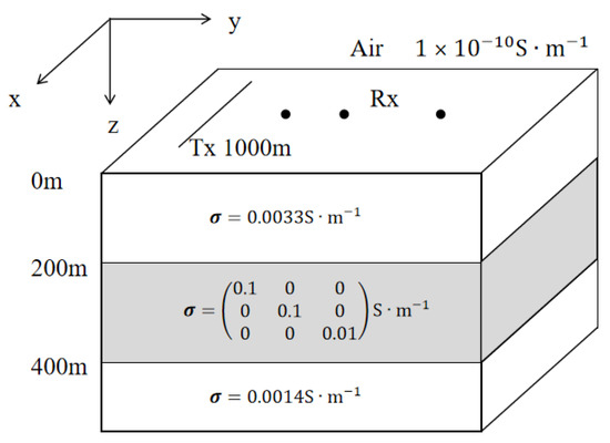
Figure 2.
Schematic diagram of the one-dimensional (1D) VTI model.
As shown in Figure 3, the and responses at the three measurement points are in good fit in shape within ~1 s. The slight error of after 0.1 s in Figure 3a is caused by the calculation accuracy between parameter conversion as the input model parameter of this algorithm is conductivity, and the input parameter of the finite volume (FV) algorithm is resistivity.
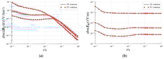
Figure 3.
Comparison of numerical results of the one-dimensional (1D) VTI model: (a) response and (b) response.
3.2. 3-D Isotropic Model
This algorithm is also applicable to the response calculation of an isotropic model. As shown in Figure 4, a typical complex isotropic vertical contact zone model was set up [33,34]. The stratum is overlain by a 50 m thick, high conductivity layer with a resistivity of 0.1 . It is then divided into different conductivity strata using the yOz vertical contact area at x = 400, where the x < 400 part is a relatively high conductivity stratum with a conductivity of 0.01 , and the x > 400 part is a low conductivity stratum with a conductivity of 0.00333 (resistivity = ). A high conductivity complex anomaly with the conductivity of 1 is immediately at the x > 400 side of the vertical contact area, which is 500 m deep, 100 m thick, and 400 m long in the y-direction (Figure 4). The coordinates of the center of the transmitting loop source are (0,50,0), the side length is 100 m, and the coordinates of the receiving points are (0,50,0), (0,150,0), (0,450,0), and (0,1050,0).
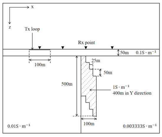
Figure 4.
Schematic diagram of the three-dimensional (3D) complex isotropic vertical contact zone model.
Figure 5 shows the impulse response of this three-dimensional (3D) model derived according to the proposed algorithm. It can be seen that matches exactly with the results of the FDM [34], and it calculated the late-time responses, which demonstrates the convergence and effectiveness of this algorithm.
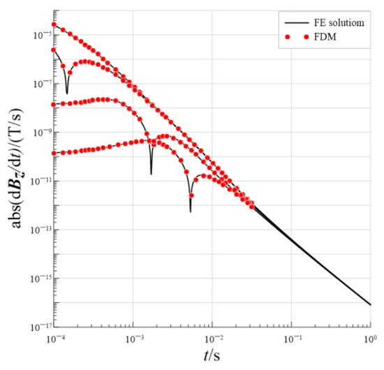
Figure 5.
Comparison of numerical results of complex isotropic model of loop source in three dimensions.
3.3. Anisotropic Half-Space Model
An anisotropic half-space airborne transient electromagnetic model of a loop source was set up [35] and validated by using the finite volume method (MFVN) [23]. As shown in Figure 6, the transmitting loop source has a side length of 20 m, is located 30 m above the ground, and emits a current of 1 A. The measurement point is located at the center of the loop and receives the response of the derivative of the vertical magnetic field component with respect to time (Figure 6). The dip angle of the stratum were set as 0° and 90°, and the ground resistivity was set to and .
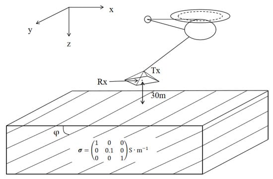
Figure 6.
Anisotropic half-space model.
As shown in Figure 7, the results of the proposed algorithm for the above anisotropic models exactly matches the results calculated using the MFVN [23] within s, which verifies the applicability of this algorithm and ensures the accuracy of the subsequent calculations.
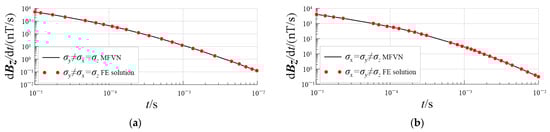
Figure 7.
Comparison of numerical results of the three-dimensional (3D) anisotropy model of the loop source: (a) y-axis direction and (b) z-axis direction.
4. Surface—Borehole TEM Response Study of Electrically Anisotropic Media
4.1. Principal Axis Anisotropic Strata
As shown in Figure 8, a stratum model was set up, and the borehole was located at the origin with a diameter of 10 cm. It was 1500 m deep and filled with mud. The long conductor source was deployed on the ground along the y-axis direction (100 m long and 1000 m from the borehole), and the measurement point was located at −500 m in the borehole. The anomaly body was 100 m long, 100 m wide, and 50 m high and was located 30 m away from the measurement point in the x-axis direction. The specific model parameters are shown in Figure 8.
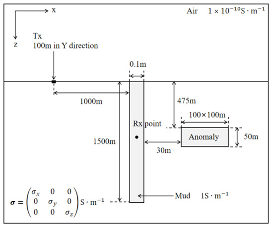
Figure 8.
Schematic diagram of the surface–borehole anisotropic transient electromagnetic method logging model.
A free tetrahedral mesh that fits a complex geological model well was used in the meshing, and the mesh size was reduced, and the number of meshes was increased at the transmitting long conductor, in-hole measurement points, and the anisotropic anomaly to improve the accuracy. Triangular meshes centered at the origin were used from the hole-mouth plane to the borehole wall and down to the whole borehole space. The complete mesh contained 3,227,084 domain elements, 88,062 boundary elements, and 20,424 edge elements (Figure 9). The calculations were performed on one node of the computer cluster, which has 20 cores, and this took approximately 40 min.
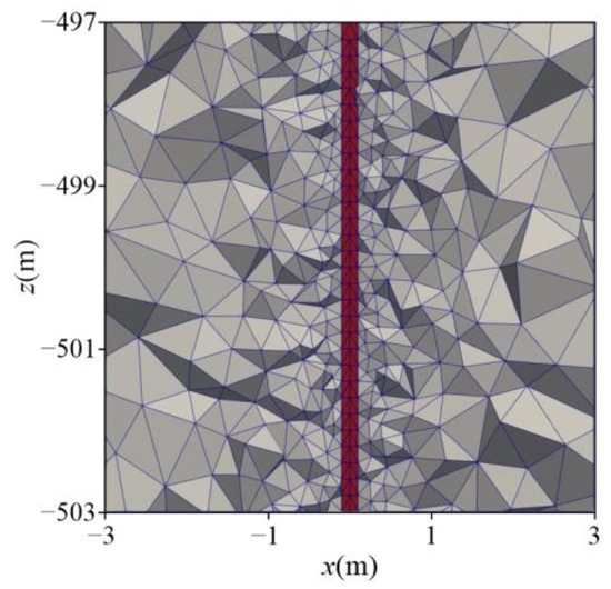
Figure 9.
Schematic diagram of meshing.
The principal axis anisotropy model and conductivity parameters are shown in Figure 10. The conductivity of the anisotropic stratum in the x-axis, y-axis, and z-axis directions was set as , and the conductivity in the remaining principal axis directions was changed to . The effects of the changes in the anisotropic stratum in the different principal axis directions were compared.
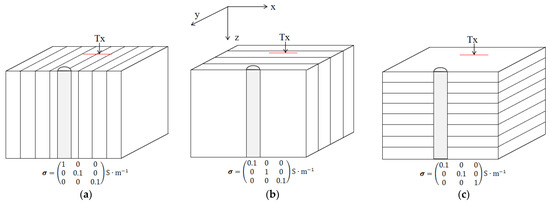
Figure 10.
Schematic diagram of the main axis anisotropic conductivity model: (a) x-axis direction, (b) y-axis direction, and (c) z-axis direction.
Figure 11 shows a comparison of the electromagnetic field response curves when the transmitting conductor is along the y-axis direction and the measurement point is (0,0,−500). When the stratum is anisotropic with a high conductivity in the x-axis direction, the electric field components E and are most significantly affected. When the stratum is anisotropic in the x-axis direction, except for the reverse change in the amplitude of , the other electric field components vary over time with the same pattern as when the stratum is isotropic. The amplitudes of the electric field components in the three directions change abruptly within ~ s, with and changing the most. changes abruptly and its pattern within ~ s is consistent with that when the stratum is isotropic. Its amplitude also changes abruptly, with and changing the most.
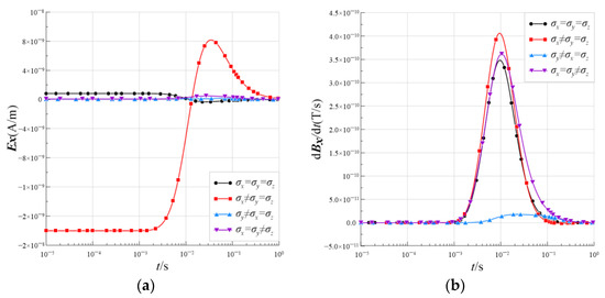
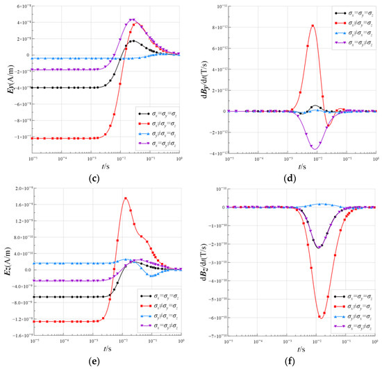
Figure 11.
Response of anisotropic strata with different principal axes: (a) response, (b) response, (c) response, (d) response, (e) response, and (f) response.
When the stratum is anisotropic in the y-axis direction, the amplitudes of and change slightly, and the response variation of is more obvious. All three components of the magnetic field response are significantly different from those of the isotropic stratum, their amplitude changes are much smaller than those if the isotropic stratum response within ~ s, and the response of even exhibits reverse growth.
When the stratum is anisotropic in the z-axis direction, both the electric and magnetic field responses differ less from those of the isotropic stratum. The response changes in and are small, and the variation in the electric field response with time is generally consistent with that of the isotropic stratum. The response curves of and are consistent with those of the isotropic stratum, but the response of varies significantly within ~ s and appears to grow in the reverse direction.
4.2. Principal Axis Anisotropic 3-D Anomaly
As shown in Figure 12, an anisotropic three-dimensional (3D) anomaly (specific parameters are shown in Figure 8) is set up. Its principal axis anisotropic conductivity tensor is , and the ground conductivity of the isotropic medium is . A measuring line of 200 m in length is set in the well, with a spacing of 10 m between the measuring points. The effects of the anisotropic anomaly in different principal axis directions are compared.
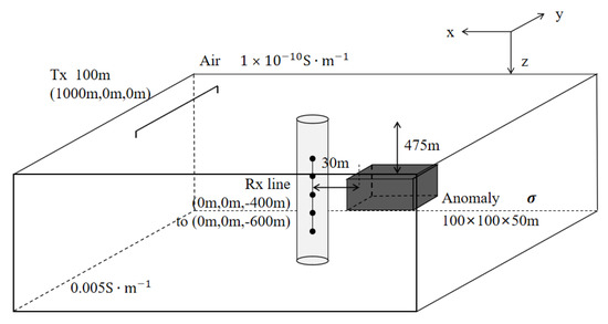
Figure 12.
Schematic diagram of the anisotropic anomaly model.
As Figure 13 shows, the responses in the different principal axis directions, and the anisotropic anomaly, are located 30 m from the measurement point (0, 0, −500 m) in the lateral direction. When an anisotropic anomaly exists next to the borehole, the response of changes with time in the same pattern as that of the isotropic stratum, but when the anisotropic principal axis direction of the anomalous body changes, the response amplitude of changes significantly in advance.
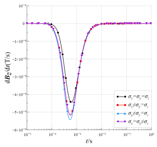
Figure 13.
response of anisotropic anomalies at point (0, 0, −500 m).
As shown in Figure 14, the response of anisotropic anomalies varies with depth in a different way compared to isotropic anomalies. Specifically, only the response of the anisotropic anomaly along the y-axis is prominently affected by depth, whereas the anisotropic anomalies along other directions show responses similar to isotropic anomalies. This suggests that the influence of anisotropy differs according to the direction being measured. Moreover, this pattern of variation is similar to that observed in the time-domain response shown in Figure 13. Both indicate that the influence of anisotropy is not only dependent on the properties of the material being measured, but also on the direction and time of the measurements. Therefore, in geophysical exploration, comprehensive analysis and interpretation based on specific circumstances are necessary to obtain more accurate information about subterranean structures.
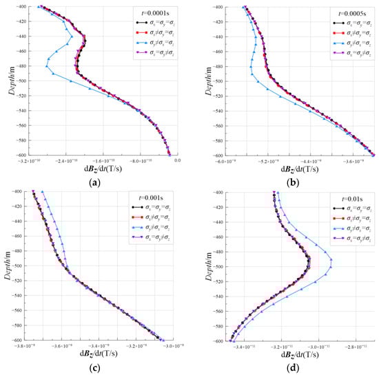
Figure 14.
response of anisotropic anomalies varies with depth at different times: (a) t = 0.0001 s, (b) t = 0.0005 s, (c) t = 0.001 s, and (d) t = 0.01 s.
5. Discussion
Through calculation and analysis of the response based on the three-dimensional (3D) principal axis anisotropy model, in surface–borehole transient electromagnetic logging, the electromagnetic field response is most significant in the horizontal plane when the high conductivity direction is perpendicular to the long conductor transmitting source, i.e., the x-axis anisotropic stratum. The response amplitude changes significantly compared to the isotropic stratum in the same situation. The amplitude of the electromagnetic field response of the y-axis anisotropic stratum changes slightly with time when the high conductivity direction of the principal axis anisotropy is parallel to the long conductor transmitting source, but the magnetic field response can be clearly distinguished from that of the isotropic stratum. The response of the anisotropy in the vertical principal axis direction varies little and is sometimes difficult to distinguish from the isotropic stratum, but the response in a particular direction is reversed.
When an anisotropic anomaly exists in an isotropic stratum, the anisotropic anomaly in the different principal axis directions only changes the magnitude of the response at the measurement point in the borehole, and it is not easily distinguished from the response of the isotropic stratum. We will investigate the relationship between the electromagnetic response of anisotropic stratum and the direction of the transmitting long conductor, the anisotropic direction of the stratum, and anomalies in a subsequent study.
Author Contributions
Conceptualization, Y.M. and L.Z.; methodology, L.Y.; software, X.W.; validation, H.L., Y.M. and X.W.; formal analysis, L.Z.; investigation, L.Y.; resources, H.L.; data curation, H.L.; writing—original draft preparation, H.L. and Y.M.; writing—review and editing, Y.M.; visualization, H.L.; supervision, L.Z.; project administration, Y.M.; funding acquisition, L.Y. and L.Z. All authors have read and agreed to the published version of the manuscript.
Funding
This research was funded by the National Natural Science Foundation of China (42274103, 42030805) and the Foundation Project (PI2021-03) of the Key Laboratory of the Ministry of Education (Yangtze University) of Petroleum Resources and Prospecting Technology.
Data Availability Statement
The data used to support the findings of this study are available from the corresponding author upon request.
Conflicts of Interest
The authors declare no conflict of interest.
References
- Zang, D.F.; Zhu, L.F.; Zhang, F.M.; Sheng, J.G.; Sheng, Y.J.; Wang, Z.L. Theory Study for Transient Electromagnetic Logging III: Electromagnetic Wave. Well Logging Technol. 2014, 38, 530–534. [Google Scholar]
- Dang, R.R.; Qin, Y.; Xie, Y.; Wang, H.N. Study of 3-C induction log system. Oil Geophys. Prospect. 2006, 4, 484–488. [Google Scholar]
- Yi, H.C. Study on the electromagnetic response characteristics of ground-well transients. Geophys. Geochem. Explor. 2018, 42, 970–976. [Google Scholar]
- Gao, J. Experimental study on transient electromagnetic logging method. Energy Technol. Manag. 2016, 41, 179–180. [Google Scholar]
- Bailey, J.; Lafrance, B.; McDonald, M.A.; Fedorowich, S.J.; Kamo, S. Mazatzal Labradorian-age ductile deformation of the South Range Sudbury impact structure at the Thayer Lindsley mine, Ontario. Can. J. Earth Sci. 2004, 41, 1491–1505. [Google Scholar] [CrossRef]
- Molnar, F.; Watkinson, D.H.; Jones, P.C. Fluid inclusion evidence for hydrothermal enrichment of magmatic ore at the contact zone of the Ni-Cu-platinum-group element 4b Deposit, Lindsley Mine, Sudbury. Can. Econ. Geol. 1997, 92, 674–685. [Google Scholar] [CrossRef]
- Deng, X.H.; Zhang, J.; Wu, J.J.; Wang, X.C.; Yang, Y. Technology design. In Protocols of Surface-Borehole Transient Electromagnetic Method, 1st ed.; China Geological Survey, Ministry of Natural Resources: Beijin, China, 2019; Volume 5, pp. 2–3. [Google Scholar]
- Klein, J.D.; Martin, P.R.; Allen, D.F. The petrophysics of electrically anisotropic reservoirs. Log Anal. 1997, 38, 25–36. [Google Scholar]
- O’Brien, D.P. Electromagnetic fields in an N layer anisotropic half space. Geophysics 1967, 4, 668–677. [Google Scholar] [CrossRef]
- Weiss, C.J.; Newman, G.A. Electromagnetic induction in a fully 3-D anisotropic earth. Geophysics 2002, 67, 1104–1114. [Google Scholar] [CrossRef]
- Pek, J.; Santos, F. Magnetotelluric impedances and parametric sensitivities for 1-D anisotropic layered media. Comp. Geosci. 2002, 28, 939–950. [Google Scholar] [CrossRef]
- Deng, S.G.; Liu, T.L.; Wang, L.; Wang, Z.; Yuan, X.; Zhang, P.; Cai, L. Analytical solution of multicomponent induction logging response in biaxial anisotropic medium. Chin. J. Geophys. 2020, 63, 362–373. [Google Scholar]
- Liu, Y.H.; Yin, C.C.; Cai, J.; Huang, W.; Ben, F.; Zhang, B.; Qi, Y.; Qiu, C.; Ren, X.; Huang, X.; et al. Review on research of electrical anisotropy in electromagnetic prospecting. Chin. J. Geophys. 2018, 61, 3468–3487. [Google Scholar]
- Li, H.; Xue, G.Q.; Zhong, H.S.; Di, Q.Y. Joint inversion of CMP gather og multi-channel transient electromagnetic data. Chin. J. Geophys. 2016, 59, 4439–4447. [Google Scholar]
- Xu, S.; Zhao, S. Finite element method solutions for geodetic electromagnetic fields in two-dimensional anisotropic geoelectric sections. Earthq. Sci. 1985, 1, 80–90. [Google Scholar]
- Yu, L.; Evans, R.L.; Edwards, R.N. Transient electromagnetic responses in seafloor with triaxial anisotropy. Geophys. J. Int. 1997, 129, 292–304. [Google Scholar] [CrossRef]
- Wang, C.X.; Zhou, C.; Chu, Z.; Wei, Y.; Jin-Song, S. Modeling of electromagnetic responses in frequency domain to electrical anisotropic formations. Chin. J. Geophys. 2006, 6, 1873–1883. [Google Scholar]
- Sun, X.Y.; Nie, Z.P.; Zhao, Y.W.; Li, A.Y.; Luo, X. The electromagnetic modeling if logging-while-drilling tool in tilted anisotropic formations using vector finite element method. Chin. J. Geophys. 2008, 51, 1600–1607. [Google Scholar]
- Chen, G.; Wang, H.; Yao, J. Modeling of electromagnetic responses of 3-D electrical anomalous body in a layered anisotropic earth using integral equations. Chin. J. Geophys. 2009, 52, 2174–2181. [Google Scholar]
- Dennis, Z.R.; Cull, J.P. Transient electromagnetic surveys for the measurement of near-surface electrical anisotropy. J. Appl. Geophys. 2012, 76, 64–73. [Google Scholar] [CrossRef]
- Yan, L.; Zhou, L.; Xie, X.; Wang, Z.G. The Transient electromagnetic responsein of electrical anisotropic reservoir model. Chin. J. Eng. Geophys. 2014, 11, 346–350. [Google Scholar]
- Wang, Y.X. Study on the 1-D Positive Inversion Method of Electrical Source Transient Electromagnetism in Anisotropic Media. Master’s Thesis, University of Electronic Science and Technology of China, Chengdu, China, 2019. [Google Scholar]
- Zhou, J.M.; Liu, W.T.; Li, X.; Qi, Z.; Liu, H. Research on the 3D mimetic finite volume method forloop-source TEM response in biaxial aniso-tropic formation. Chin. J. Geophys. 2018, 61, 368–378. [Google Scholar]
- Liu, Y.; Hu, X.; Peng, R.; Yogeshwar, P. 3D forward modeling and analysis of the loop-source transient electromagnetic method based on the finite-volume method for an arbitrarily anisotropic medium. Chin. J. Geophys. 2019, 62, 1954–1968. [Google Scholar]
- Liu, Y. Three-Dimensional Anisotropy Forward and Analysis of Time-Domain Electromagnetic Method. Ph.D. Thesis, China University of Geosciences, Beijing, China, 2020. [Google Scholar]
- Guo, J.L.; Jiang, T.; Guo, H. Characteristics of axial anisotropic borehole transient electromagnetic three-component response. J. Earth Sci. Environ. 2020, 42, 737–748. [Google Scholar]
- Guo, J.; Gao, X.; Hou, Y. Research on three-component responses characteristics of axial anisotropy tunnel-hole transient electromagnetic. Coal Geol. Explor. 2022, 50, 52–62. [Google Scholar]
- Yin, C.C. Geoelectrical inversion for a one-dimensional anisotropic model and inherent non-uniqueness. Geophys. J. Int. 2010, 1, 11–23. [Google Scholar] [CrossRef]
- Pek, J.; Santos, F. Magnetotelluric inversion for anisotropic conductivities in layered media. Phys. Earth Planet. Inter. 2006, 158, 139–158. [Google Scholar] [CrossRef]
- Um, E.S.; Harris, J.M.; Alumbaugh, D.L. 3D time-domain simulation of electric-field approach. Geophysics 2010, 75, 115–126. [Google Scholar] [CrossRef]
- Yu, C. Introduction of PARDISO Solution Method for Large-Scale Sparse Matrix; Intel Asia Pacific Research and Development Center: Shanghai, China, 2002. [Google Scholar]
- Liu, Y.; Pritam, Y.; Hu, X.; Peng, R.; Tezkan, B.; Mörbe, W.; Li, J. Effects of electrical anisotropy on long-offset transient electromagnetic data. Geophys. J. Int. 2020, 222, 1074–1089. [Google Scholar] [CrossRef]
- Commer, M.; Newman, G. A parallel finite-difference approach for 3D transient electromagnetic modeling with galvanic sources. Geophysics 2004, 69, 1192–1202. [Google Scholar] [CrossRef]
- Liu, S.; Sun, H.; Li, W.; Wang, Z.; Yang, Y. New algorithm for transient electromagnetic BEDS-FDTD 3-D forward and stability verification. Chin. J. Geophys. 2023, 66, 841–853. [Google Scholar]
- Yin, C.; Qi, Y.; Liu, Y. 3D time-domain airborne EM modeling for an arbitrarily anisotropic earth. J. Appl. Geophys. 2016, 131, 163–178. [Google Scholar] [CrossRef]


Disclaimer/Publisher’s Note: The statements, opinions and data contained in all publications are solely those of the individual author(s) and contributor(s) and not of MDPI and/or the editor(s). MDPI and/or the editor(s) disclaim responsibility for any injury to people or property resulting from any ideas, methods, instructions or products referred to in the content. |
© 2023 by the authors. Licensee MDPI, Basel, Switzerland. This article is an open access article distributed under the terms and conditions of the Creative Commons Attribution (CC BY) license (https://creativecommons.org/licenses/by/4.0/).