Abstract
The operation of a froth flotation column can be described by a nonlinear convection–diffusion partial differential equation that incorporates the solids–flux and drift–flux theories as well as a model of foam drainage. The resulting model predicts the bubble and (gangue) particle volume fractions as functions of height and time. The steady-state (time-independent) version of the model defines so-called operating charts that map conditions on the gas and pulp feed rates that allow for operation with a stationary froth layer. Operating charts for a suitably adapted version of the model are compared with experimental results obtained with a laboratory flotation column. Experiments were conducted with a two-phase liquid–bubble flow. The results indicate good agreement between the predicted and measured conditions for steady states. Numerical simulations for transient operation, in part for the addition of solid particles, are presented.
1. Introduction
Froth flotation is the most important concentration operations in mineral processing and is widely used for the recovery of valuable minerals from low-grade ores (cf. [1], ([2], Chapter 12) or ([3], Part 7)). This unit operation is an important stage particularly for copper mining in Chile. The flotation process selectively separates hydrophobic materials (that are repelled by water) from hydrophilic (that would be attracted to water), where both are suspended in a viscous fluid. It is well known that a flotation column works as follows: gas is introduced close to the bottom and generates bubbles that rise through the continuously injected pulp that contains the solid particles.
The hydrophobic particles (the valuable mineral particles) attach to the rising bubbles, forming froth that is removed through a launder. The hydrophilic particles (slimes or gangue) do not attach to bubbles but settle to the bottom (unless they are trapped in the bulk upflow) and are removed continuously as flotation tailings. Close to the top, additional wash water can be injected to assist with the rejection of entrained impurities and to increase the froth stability [1,4,5]. This unit operation is particularly suitable for processing low-grade ores, such as copper ores in Chilean deposits; however, this requires huge amounts of process water.
Since water is a scarce resource for most economic activity in Chile—in particular in the desert areas where most mines are located—the improvement of the scientific understanding of flotation processes and the development of suitable tools for the design, simulation and control of flotation devices is of critical economical, ecological and societal importance. This situation has motivated collaborative research between applied mathematicians and metallurgical engineers at Universidad de Concepción.
Modelling flotation and developing strategies to control this process are research areas that have generated many contributions [6,7,8,9,10,11,12,13,14,15]. The development of control strategies requires dynamic models along with a classification of steady-state (stationary) solutions of such models. These models should focus on the separation process aligned with gravity and are, therefore, spatially one-dimensional. (In fact, we wish to avoid the additional computational effort associated with spatially two- or three-dimensional models, mostly based on computational fluid dynamics (CFD) that also involve the solution of additional equations for the motion of the mixture; we refer to [16] for a review on CFD-based models of flotation).
The sought unknowns are the volume fractions of gas (bubbles), liquid, and possibly solid particles as functions of both time and spatial position, so that the resulting governing equations are partial differential equations (PDEs). With the aim of developing controllers, some authors [9,10,11,12] used hyperbolic systems of PDEs for the froth or pulp regions coupled to ordinary differential equations (ODEs) for the lower part of the column. These include the attachment and detachment processes; however, with their approaches, the phases seem to have constant velocities, which is not in agreement with the established drift–flux theory [17] that establishes that the velocity of a unit of the disperse phase (droplet, bubble or particle) is a function of the local volume fraction (or concentration). Nonlinear dependence of the phase velocities on the volume fractions gives rise to discontinuities in the concentration profiles, which was confirmed experimentally [6].
Narsimhan [18] showed realistic conceptual transient solutions of an initially homogeneous bubble–liquid suspension. The rising bubbles form a layer of foam at the top, which can undergo compressibility due to gravity and capillarity. Separate equations are derived for the foam region, and boundary assumptions between regions have to be imposed. The purpose of our previous contribution [19] (see also [20]), which is utilized herein in a slightly modified form, is to let one single equation govern the bubble–liquid behaviour in the whole column under any dynamic situation without any imposed boundary conditions.
Such are automatically assumed by the PDE solutions, which satisfy the so-called entropy conditions by definitions of the PDE coefficients that are discontinuous across the feed, discharge and overflow levels of height. When solids are also fed into the column, an additional equation modelling the settling of solids outside the bubbles is needed—still without any imposed boundary conditions.
Phenomenological models for two-phase systems with bubbles rising (or, analogously, particles settling) in a liquid, are derived from the physical laws of conservation of mass and momentum [21,22]. Under certain simplifying assumptions on the stress tensor and partial pressure of the bubbles/solids, one can obtain first- or second-order PDEs involving one or two constitutive (material specific) functions, respectively. The resulting first-order PDE modelling such a separation process in a one-dimensional column of rising bubbles is a scalar conservation law
where t is time, z is a spatial position (height), is the sought volume fraction of bubbles, and
is the bubble (aggregate) batch flux density function, where is a given drift–flux velocity function. The formulations (1) and (2) are in agreement with the drift–flux theory [17]. With additional bulk flows due to the inlets and outlets of the column, that theory has mostly been used for investigations of steady states of flotation columns [5,23,24,25,26]. Models of and numerical schemes for column froth flotation with the drift–flux assumption and possibly simultaneous sedimentation have been presented in [27,28,29,30].
The analogy of the drift–flux theory for sedimentation is the established solids–flux theory [17,31,32,33]. With an additional constitutive assumption on sediment compressibility, the corresponding model becomes a second-order degenerate parabolic PDE [21]. Sedimentation in a clarifier–thickener unit is mathematically similar to column flotation. A full PDE model of such a vessel necessarily contains source terms and spatial discontinuities at both inlets and outlets. Steady-state analyses, numerical schemes, dynamic simulations and the control of such models are reported in [32,34,35,36,37].
The first-order PDE of the flotation process advanced in [28] does not include capillarity in the foam. Such effects have been studied intensively [38,39,40]; see also [13]. Solids motion in froth was investigated in [41]. A generalized model PDE that captures both the rising bubbles of low concentrations and the formation and drainage of froth at high concentration was recently presented in [19]. That article contains a generalized model when settling particles are also present in a specific flotation column with a common feed inlet for both pulp and gas.
In this contribution, we adjust the generalized drainage model to an experimental laboratory flotation column with separate inlets for gas and mixture (Figure 1), derive the so-called desired steady state (which has a foam layer in the upper part and no bubbles leaving at the underflow) and find a single set of parameters in the model that qualitatively captures several steady state experiments. The numerical simulations presented here are made with the numerical method in [19] and adapted to the setup of the pilot column (Figure 1).
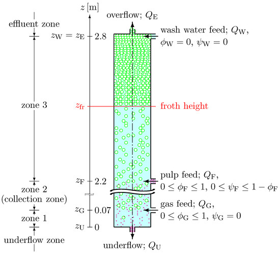
Figure 1.
Conceptual drawing of the model of the pilot flotation column: (left) denomination of zones, (middle) height axis (z-axis) showing the locations of the feed and discharge levels and (right) schematic of the column. The green open circles and solid magenta dots represent bubbles and hydrophilic particles (bubbles and particles are not drawn to scale), respectively. The information to the right indicates the overflow rate, volume feed rates and concentrations and the underflow volume rate along with limitations that the feed concentrations must satisfy. The denomination of zone 2 as a “collection zone” is common in mineral processing, although the process of collection (the adhesion of hydrophobic particles to bubbles) is not part of the model.
2. Materials and Methods
2.1. Pilot Flotation Column and Experimental Setup
The experiments were conducted at the laboratory of the Department of Metallurgical Engineering of Universidad de Concepción with a laboratory-scale flotation column; see Figure 2a. This column was made of acrylic to visualize the internal phenomena that occur in both the collection and cleaning areas. The column had a volume of 54.7 L and an interior diameter of 6 inches so that its cross-sectional area was and was high (see Table 1).

Table 1.
Dimensions of the pilot flotation column.
The air was injected from the lower central part of the column through a sparger whose pores were in diameter. The locations of the inlets and outlets are detailed in Figure 1. The column was instrumented as shown in Figure 2b. For the tests, the use of solids was not considered, the only reagent to be used was a mix (1:1) of MIBC (methyl isobutyl carbinol, an organic chemical compound used primarily as a frother in mineral flotation) and polyglycol as a frother at a dosage of 100 g/L of water.

Figure 2.
(a) Photograph of the laboratory column and (b) schematic of the piping and instrumentation devices (P & ID). See Table 2 for explanation.
Table 2.
Legend of the P & ID schematic (Figure 2, right).
Figure 2.
(a) Photograph of the laboratory column and (b) schematic of the piping and instrumentation devices (P & ID). See Table 2 for explanation.

2.2. Experimental Determination of Stability Regions
We performed five steady-state experiments; see Table 3. There are 36 data points in the interval of the underflow velocity . The resulting upper and lower limits of within which a pulp–froth interface is present in zone 3 are presented in Figure 3 and Figure 4. The enclosed region between the two curves may be called the stability region since, for values of therein, a stable pulp–froth interface in zone 3 was observed experimentally. On the other hand, for choices of , outside that region, unstable operation was observed, which means that either no froth layer was produced at all or that the froth layer reached into zone 2 and possibly that bubbles left through the underflow.
Table 3.
Overview of the five steady-state experiments.
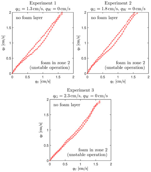
Figure 3.
Experiments 1–3 (no wash water added): stability regions enclosed between two curves formed by points in the plane.
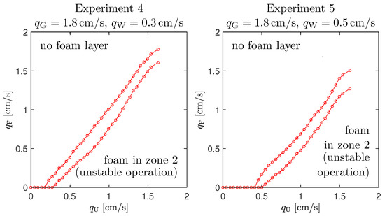
Figure 4.
Experiments 4 and 5 (with wash water added): stability regions enclosed between two curves formed by points in the plane.
A stable pulp–froth interface in zone 2 is a valid stationary solution (corresponding to a mode of operation in which the pulp feed acts as a submerged feed source), but such steady states are very difficult to control, and we, therefore, address them as “unstable operation”. This procedure is consistent with the theoretical steady-state analysis of [19] (see also Section 3.4) and in particular the construction of operating charts in which any theoretical situation in which the froth level cannot be accommodated within zone 3 is deemed “unstable,” independently of whether the parameters permit a froth layer within zone 2 or not (i.e., bubbles leave through the underflow).
In order to ensure the reproducibility of the experiments, the tests were performed in duplicate and randomly, and we report only the average values. The standard deviation of the tests was less than 5%.
3. Theory
3.1. Mathematical Model
The governing model combines the setup with separated inlets for gas and the pulp formulated in [27] with the approach of describing foam drainage developed in [19]. The model is formulated as a three-phase model formed of the gas bubbles and (hydrophilic gangue) solid particles as primary and secondary disperse phases that move in the fluid that forms the continuous phase.
The present experimental support refers to a two-phase flow model only, but for illustrative purposes, we present one numerical simulation corresponding to a (hypothetical) solids feed. The three phases and their (dimensionless) volume fractions are the fluid , the solids and the bubbles (aggregates) , where . A mixture of fluid and solid particles is addressed as a suspension. The volume fraction of solids within the suspension that fills the interstices between bubbles is defined by
The system of PDEs that governs the evolution of and can be formulated as
Apart from the variables introduced in the context of (1) and above, here, is the cross-sectional area of the tank, and and are convective flux functions that depend discontinuously on z at the locations of the gas inlet (), the pulp feed inlet (), the wash water inlet (), the underflow outlet () at the bottom and the overflow outlet () at the top; see Figure 1.
The system (3) is valid for and all z, . The characteristic function indicates the interior of the tank:
The nonlinear function D, see Figure 5, models the capillarity present when bubbles are in contact and is given by
where the function d (introduced in [19] and specified later in this work) is assumed to satisfy
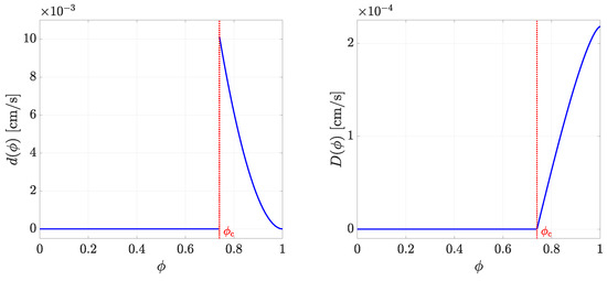
Figure 5.
Functions (left) and (right) modelling the capillarity. In both figures, we set .
Consequently, at each point where , there holds , and therefore (3) degenerates at such points into a first-order system of conservation laws of hyperbolic type. (Precise algebraic definitions of J, and d are provided further below).
The last term on the right-hand side describes three singular sources located at the level , , where is the corresponding volume feed rate (as a given function of time) and and are the respective bubble and solids feed concentrations. Of course, under normal circumstances the solids feed concentration at the gas inlet should be zero (), the bubble feed concentrations at the pulp feed inlet should be zero (), and the concentrations of both disperse phases at the wash water inlet should be zero (, ). Outside the tank, the mixture is assumed to follow the outlet streams. Consequently, boundary conditions are not needed; the conservation of mass determines the outlet volume fractions in a natural way.
Since the wash water is located at the top of the column, we have . Thus, the interior of the flotation column can be subdivided into three zones. In what follows, for the ease of discussion, we refer to the z-subintervals as “the effluent zone,” as “zone 3,” as “zone 2,” as “zone 1” and as “the underflow zone.”
Applying the conservation of mass to each of the three phases, introducing the volume-average velocity, or bulk velocity, of the mixture q and the relative velocities of both the aggregate suspension and the solid–fluid, Bürger et al. [28] derived a PDE model similar to (3) without the capillarity function and assuming that there is one joint inlet for both the pulp and the gas. Extending this approach to the present setup, we obtain the flow rates (velocities) in and out of the flotation column
The drift–flux and solids–flux theories utilize constitutive functions for the aggregate upward batch flux and the solids batch sedimentation flux
where is the hindered–settling function. For simplicity, we employ the Richardson–Zaki expression [42]
and is the velocity of a single particle. In the underflow and effluent zones, all phases are assumed to have the same velocity, i.e., they follow the bulk flow. Then, the total convective fluxes for and are given by
with the zone-settling flux functions (positive in the direction of sedimentation, that is, decreasing z)
Here, the batch drift–flux function is given by (2), where is given by
Here, is the constant velocity of a single bubble in liquid, and is a dimensionless constant. The expression in the first case of (10) is valid as long as the bubbles are not all in contact with each other. This contact is assumed to occur whenever exceeds the critical concentration . The expression in the second case of (10) is derived from a compatibility condition that makes it possible to express the drainage velocity of the liquid in the froth relative to the bubbles with respect to gravity and dissipation in terms of and the dimensionless constant .
The latter emerges from empirical connections between the radius of the Plateau borders in the foam, the radius of the bubbles and the volume fraction of the liquid in the foam ; see [19] for all details. The function arising in (5), and which describes capillarity, is given by
where is a capillarity-to-gravity constant present in the froth when and involving, among others, the surface tension of water; see [19]. In light of (11), we obtain
where , and we reconfirm the property (5). Finally, we define the total convective flux for the solids appearing in the governing system (3) by
3.2. Reduced Model for Two-Phase Flow of Bubbles in Liquid
The description provided so far refers to the full model that involves a feed of both gas bubbles and solids in the water. The currently available experimental data, however, are, for the moment, limited to a two-phase gas–liquid system; measurements of the system behaviour with solids feed are currently being made and will be presented in forthcoming work. We here focus on the dynamics of the gas–liquid system considering the effects of froth drainage. Furthermore, since the pilot column is cylindrical, we assume that A is constant (we utilize as indicated in Section 2.1).
Under this assumption (that is, the presence of particles is neglected) the model reduces to the scalar PDE
where we define the velocities
and the definitions , (8), , (12) and remain in effect. These and other variables have the range of values given in Table 4.
Table 4.
Range of parameters according to the literature (typical values employed in [43,44,45,46,47]) and used in the present work.
3.3. Numerical Method
The numerical method used for the solution of the complete model is outlined, and in part analysed, in [19]. It is based on subdividing the computational domain, corresponding to a z-interval that encloses the tank (that is, the interval into a number N of layers (subintervals) of equal height , and time is discretized through time points , . Without entering into any details, assume that the unknowns of the scheme are and , where these quantities are approximate values of and in cell j at time , respectively. The general scheme can then be written in the form
We refer to [19] for all details regarding the precise algebraic forms of the functions and , which are chosen in such a way that (14) represents a consistent finite difference approximation of the system (3) and all ingredients outlined in Section 3.1. While any specific information is omitted here (for brevity), the general formulation (14) is useful to indicate some particular properties of the numerical scheme of [19]: first, the scheme is explicit, that is, from the given initial values and , , one successively calculates and , , then and , and so on for .
Furthermore, the system (3) is triangular, which means that the first equation, the PDE for the update of , contains, apart from , only terms that depend on known functions and and its z-derivatives. On the contrary, the second PDE, for the update of , contains, apart from , terms that depend on both and . Thus, the bubble volume fraction can be updated independently from the solids volume fraction , which is also reflected in the different arguments of and in (14).
Consequently, the first update formula of (14) is a valid numerical scheme for the one-equation reduced model outlined in Section 3.2. Furthermore, the functions and are based on particular numerical fluxes that satisfy the so-called monotonicity property, which ensures that, if the initial values are physically relevant, i.e.,
is in effect for , then the same property is valid for all . The latter property makes the approach of [19] interesting for practical applications. That said, for a given layer thickness , one needs to choose the time step in such a way that the Courant–Friedrichs–Lewy (CFL) condition is satisfied. Such a condition also ensures that the numerical approximations converge (as ) to an exact solution of the model as is outlined in [48].
3.4. Desired Steady States for the Two-Phase System
There are many different steady-state solutions of (13) depending on the values of all the feed velocities in and out of the column and volume fractions of the inlets. We are interested in the desired steady states, which means that no bubbles leave through the underflow, and there is a froth level. This is the interface in zone 3 (above the feed inlet ) above which the froth is located. Similar desired steady states were presented in [19] for the general model (3) but for the special case when the gas and slurry feed inlets coincide.
We here follow the description in [19], which, in turn, refers to [28,49], and we leave out the mathematical details. The latter involves uniqueness issues and entropy conditions for discontinuities of the solution . Such discontinuities arise in three different situations, namely: (1) in regions where and the PDE is hyperbolic; (2) across the discontinuity from a lower concentration up to the critical concentration , beyond which the PDE is parabolic; and (3) across the z-positions of inlet and outlets, where the total flux function of (13) is discontinuous (with respect to z).
We directly let , since there is no gas in that feed inlet. If we write the delta symbol on the right-hand side of (13) formally as , where
is the Heaviside function, then time-independent solutions of (13) satisfy the second-order ODE
This ODE can be integrated with respect to z to yield
where the constant mass flux per area unit M can be determined by considering (15) outside the tank—that is, for setting either or , such that , and hence
Since, in a desired steady state, and , (16) implies that the effluent concentration is given by
In zone 2, we want a solution that satisfies ; hence, , and choosing in (15), we obtain
where writing out the dependence of on is convenient when investigating the dependence of steady-state solutions on the bulk velocities. We denote by the smallest solution of (18), which is thus the constant solution in zone 2. The conditions for this solution are
where is the maximum point of for given and the positive zero of ; see [19] for exact definitions. The analogous conditions can be found in [19].
In Figure 6 (left), we can see a possible steady-state value for zone 2, with and satisfying both conditions (19) and (20). Another steady state with high volume fractions greater than in the entire zone 2 could, in some cases, be possible theoretically; however, this is not a desirable steady state. Here, and in the rest of the text, will denote the local minimum point greater than the inflection point of , analogously for ; see [19] for details.
As in [19], we construct a solution in zone 3, which is
where is a constant volume fraction above and below the pulp–froth interface located at . Flux continuity and an entropy condition not detailed here yield that is the smallest solution of
which means that when . Furthermore, in (22), is the strictly increasing solution of the ODE
(see (21)), where is the unknown location of the pulp–froth interface . Thus, problem (24) defines a function from all input variables to the pulp–froth interface via (recall that is given by (17))
In Figure 6 (right), we can see a possible steady-state value for zone 3, with satisfying (23). Note that, in this case, there does not exist a steady-state value with , since the straight line given by does not intersect with the flux function for values of . Moreover, since condition (27) is not satisfied for the values of the volumetric flows chosen, the solution in zone 3 will be constant and equal to , i.e., the solution of the ODE (24) does not exist, and hence a froth layer is not possible in this scenario.
In conclusion, the desired steady state for the two-phase gas–liquid system is, thus,
In Figure 7, some desired steady states of this type are shown. This solution can only be obtained if the conditions (19), (20) and (25)–(27) are satisfied. We visualize these conditions in two-dimensional operating charts in the -plane for given , and . To exemplify, we illustrate these conditions in Figure 8 for the first steady-state experiment.

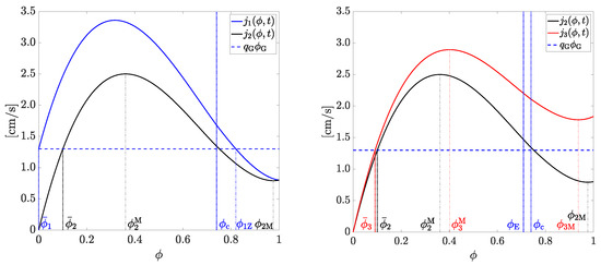
Figure 7.
Examples of desired steady states for the gas phase, given by (28). To obtain these figures, we used fixed values of , , , and , and we varied , choosing: (a) , (b) , (c) and (d) . With these values for the volumetric flows, we obtained a pulp–froth interface located at (a) , (b) , (c) and (d) , respectively, and an effluent volumetric fraction of (a) , (b) , (c) and (d) .


Figure 8.
Operating charts showing the theoretical conditions for a steady-state with a froth present in the upper part of the flotation column for the first steady-state experiment. A white region means that the condition is satisfied. The superposition of all these charts results in a white strip, which can be seen in the -plane in Figure 9 (Experiment 1). The labels (FIa), (FIb), (Froth1), (Froth2), and (Froth3) correspond the notation in [19] and to the respective inequalities (19), (20), (25), (26), and (27) in the present work.


Figure 9.
Experiments 1–3 (no wash water): Comparisons between the model with stationary conditions. Here, and in Figure 10, each -plane shows the operating chart in which the white region shows the theoretical conditions for a pulp–froth level above the feed level (cf. Figure 8). The red lines in that plane (see also Figure 3 and Figure 4) show the experimental lower and upper values of for each given , in between which, a pulp–froth level was observed. The yellow surface is the graph of the function , i.e., the estimated height of the pulp–froth interface by the model.


Figure 10.
Experiments 4 and 5 (with wash water added): comparisons between the model and experiments with stationary conditions.
Figure 10.
Experiments 4 and 5 (with wash water added): comparisons between the model and experiments with stationary conditions.

4. Results
4.1. Choice of Parameters
The model contains several parameters. We fixed and with the arguments given in [19] for a general froth and let , and be those that should be adjusted to reproduce the experiments—at least qualitatively. We thus aimed to find the same fixed values for all experiments. As stated in [28], there exist a number of methods to calculate . The generalized correlation by Wallis [50] is recommended; see [23], Appendix A for details. This correlation involves additional quantities, such as the equilibrium surface tension and the viscosity of the fluid. Its discussion is beyond our focus.
Values for normally range from 2 to 3.2. For given values of and , the constant volume fraction in zone 2 could be estimated experimentally. Equation (18) could then be used to estimate
where in our experiments. Choosing , we obtained the value cm/s, which gave qualitatively similar operating charts by the model as from the experiments. As for the capillary-to-gravity parameter involved in the modelling of the capillary effect in the froth, we found that the single value cm could be used for a qualitative description of all five steady-state experiments.
All the numerical results were obtained with a spatial discretization of computational cells, which means a spatial step size of and a time step satisfying the CFL condition.
4.2. Comparison between the Model and Experimental Stationary Data
Comparisons between the model and the five steady-state experiments can be seen in Figure 9 and Figure 10. The goal is that the region between the two experimental lines coincides with the white region of the theoretical operating chart, i.e., the -plane. The qualitative agreement between the experimental data and the model must be considered very good, considering that the theoretical model contains several idealized assumptions and several parameters whose values were taken from the literature for a general sludge. We emphasize that the same parameter values were used in the model for all experiments. The model prediction of the froth level is given by the yellow surface in each subplot of Figure 9 and Figure 10.
In Figure 11, we explain the use of the operating charts of Figure 9 and Figure 10 for the particular case of Experiment 1 (Figure 9a). For a fixed value of , we chose four values of on the line —shown in dark green in the 3D plot (Figure 11a) inside the white region of the operating chart. For each point chosen, using the correspondence , we know the estimated height of the pulp–froth interface given by the model; see Figure 11b. In Figure 11c–f, we show the graphs of the steady states for the gas phase recovered with the values of chosen, which are in accordance with the results shown in Figure 11b.
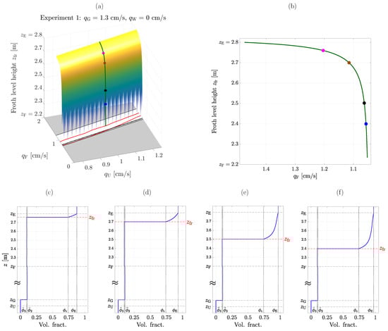
Figure 11.
Experiment 1: Example of the use of the operating charts in Figure 9 and Figure 10. (a) Enlarged view of Figure 9a. For a fixed value of , the line is marked in dark green, and four points with between and inside the white region of the operating chart were chosen. (b) Cross section of the surface for (the -axis is oriented in decreasing order for ease of comparison with plot (a)). (c–f) Steady states for the gas phase obtained with the points marked in plots (a,b). The values used in each figure are (c) , (d) , (e) and (f) .
Figure 12 shows a dynamic simulation of the model from a column initially filled with only water and with the parameters of Experiment 1. As can be seen, a steady-state solution arises with a froth layer at the top and with constant volume fractions of bubbles in each zone otherwise. In particular, the steady-state concentration in zone 2, , is slightly larger than the volume fraction in the lower part of zone 3 as the theoretical steady states predict.
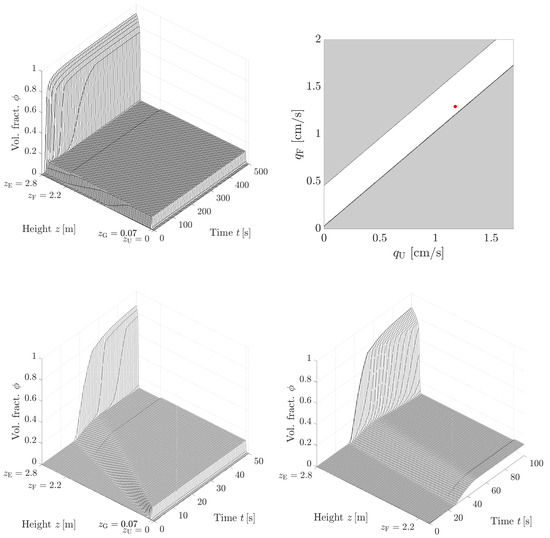
Figure 12.
First row: Numerical simulation of a fill-up process (left) and operating chart (right) of the model with parameter values of Experiment 1 and bulk velocities , which is the red point inside the white region. Second row: Zoom in time of the fill-up process during the first (left) and a zoom in space showing the top of the column, where the foam formation in zone 3 is clearly seen during the first (right).
The qualitative agreement between the model and experiments lies in the fact that both the model and the experiments confirm that it is only for a small region in the four-dimensional space of -values that a froth layer exists. Both the model and the experiments verify that, once a steady state has been found with a froth level, a small change in any of the bulk velocities will either make the froth layer be flushed out upwards or the entire column filled with bubbles, which also leave through the underflow.
4.3. Simulation of Dynamic Behaviour and a Case with a Solids Feed
4.3.1. A Dynamic Simulation of Two-Phase Bubble–Liquid Flow
We start with the tank full of only fluid at time ( for all z) when we start pumping gas and fluid, with and at the feed inlet and and at the gas inlet. We choose the flow rates
in the white region of the theoretical operating chart in Figure 13—marked in red colour. With these parameters, we obtain a desired steady state with a froth layer at the top of the column and no bubbles leaving through the underflow after about ; see Figure 13 (left).
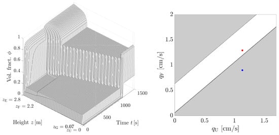
Figure 13.
Dynamic simulation of a bubble–liquid flow. (Left) Time evolution of the volumetric fraction profile of loaded gas bubbles from to . (Right) Theoretical operating chart for the simulation in Section 4.3.1. The point marked in red corresponds to and the one in blue to .
Once the system is in a steady state at , we make a step change from to . The new point chosen lies in the grey region of the theoretical operating chart—marked in blue in Figure 13 (right). As one expects after this change, the froth layer increases, and bubbles at high volume fractions fill the entire column as can be seen in Figure 13 (left). This illustrates how our model is capable of predicting changes in the system and thus is able to take the appropriate control actions. In this case, the control action leads to an undesired steady state since there are gas bubbles leaving through the underflow.
4.3.2. A Dynamic Simulation of Three-Phase Bubble–Solids–Liquid Flow
As in the previous example, the column is initially full of only fluid when we start pumping bubbles and solids with the volume fractions , , and along with fluid and wash water. We choose the flow rates
Figure 14 shows the time evolution of the volume fractions and . It can be seen that a desired steady state arises with a layer of froth at the top, while the solids are present only below the feed level where they settle to the bottom.
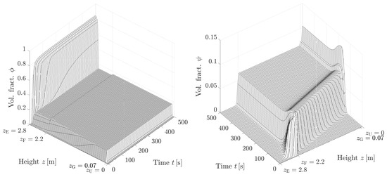
Figure 14.
Dynamic simulation of bubble–solids–liquid flow. Time evolution from to of the volume fraction profiles of bubbles (left) and solids (right).
5. Discussion
The theoretically derived PDE model automatically captures several different phenomena (hindered bubble rise, hindered settling of particles and the formation of foam) without any boundary conditions. The model predicts that a desired steady-state solution with a froth layer above the feed level is only possible in a thin region in -space. The same set of model parameters was used for all comparisons with the five experiments. The model involves nonlinearities in both the convective and diffusive parts and is strongly degenerate in the diffusive part and, therefore, gives rise to discontinuities in the concentration profiles, which was confirmed experimentally [6] (as emphasized in [19]; see also ([3], p. 915, Figure 3)).
This property is inherent to drift–flux analyses (that disregard a diffusive term that, in our context, models capillarity) (see, for instance, [5,23,24,25,27]). However, this contrasts with the approaches by Azhin et al. [11,12] and Tian et al. [9,10] that are based on linearized models and where continuity conditions and boundary conditions are imposed explicitly, and therefore continuous steady-state profiles are obtained. The qualitative agreement between our model and the experiments is interesting and shows the possibilities for further investigations and model calibration. A reason for the discrepancies between the model output and the experimentally determined regions in the operating charts, when a stationary froth level in zone 3 is possible (see Figure 9), is the following.
Above the white region in each theoretical operating chart, i.e., the -plane, the combination of the bulk velocities are such that no layer of foam can exist according to the PDE model. In decreasing the value of for fixed , and such that the point lies in the white region, then a froth level is possible in zone 3 (). In the upper strip of the white region, the model predicts a froth level (the yellow surface) close to the effluent level , which means a very thin layer of froth. It may well be that such thin froth layers were not registered as valid in the experiments. It is therefore natural that the upper experimental red line lies some distance below the upper line of the white region.
The fact that the lower red line, at least when wash water is present, lies further down in the grey region, means that a froth level is observed close to, but above, the feed level , i.e., almost the entire zone 3, is filled with froth. The theoretical model does not fully capture this behaviour and predicts that, for points below the white region, the entire zone 3 is filled with foam, and there are possibly bubbles dragged down to the underflow. This discrepancy between the model and experiments near the location of the pulp–froth interface when wash water is applied should be further investigated.
In the model development in [19], several reasonable assumptions (partially verified by reported experiments) for the drainage in the froth were assumed to hold for volume fractions close to but above the critical concentration in order to obtain a unified model. It appears that further modelling is needed for the behaviour near the pulp–froth interface. That said, we suggest that that the foam model and the description of that interface by a critical concentration is consistent with the approach by Neethling and Cilliers [39] (which is further elaborated, e.g., in [40]).
6. Conclusions
The conclusions arising from the specific findings of our theory, simulations and experiments are outlined in Section 5. In summary, we can say that the model (3), plus constitutive equations and specifications of control functions, is based on several existing theories (the drift–flux and solids–flux models as well as the model of foam drainage) and lays the ground for a complete simulator of a flotation column in one space dimension without the need to impose boundary conditions or track, for instance, the pulp–froth interface. We once again refer to [19] for an exposition of all technical details. Let us emphasize here the following aspect.
Our previous work [19,28,29], as well as the transient simulations presented herein, have demonstrated that the (theoretical) steady-state theory is consistent with (numerical) simulations of transient scenarios in the sense that steady states are assumed precisely when the various parameters are chosen such that the point lies in the “white region” of the corresponding operating chart. In addition, the model does not catastrophically “break down” when the desired steady-state conditions are violated but makes precise predictions of the “unwanted” behaviour (e.g., bubbles leave through the underflow as seen in Figure 13). This consistency is internal to the mathematical model; however, the comparison with experimental results conducted in this work are the first results that indicate that the model is also consistent with experimental observations. That said, further experiments and comparisons with simulations should be conducted with a focus on transient behaviour and involving solids.
With respect to the potential use of the model in real flotation practice (for instance, to optimize the flotation performance) we mention that the model presented is an advancement of the phenomenological models currently reported in relation to the description of the foam level within the column as well as the gas hold-up. Although it does not yet consider the attachment and detachment mechanism of particles to bubbles, the model is reasonably accurate in determining the stable operating zones, which would allow its use as a complement to current control systems [7,8,10,12,13,14,15,45]. Examples of control systems based on the involved phenomenological models (coupled PDEs) have been reported and used in other unit operations [32,51,52,53,54,55,56].
The present approach captures the multiphase hydrodynamics of aggregates (bubbles) and gangue particles in the column but does not model the aggregation process itself (that is, the attachment of hydrophobic (valuable) particles to gas bubbles). That process usually takes place in the collection zone (zone 2 in Figure 1). To add realism and to explore the interdependence of velocities and reaction kinetics, the flotation model (3) should be extended to include the process of attachment of hydrophobic (valuable) particles. One option consists of considering the valuable and gangue particles as two independent disperse solid phases (while the present approach only includes the gangue) and adding another field variable that describes the local state of aggregation. This procedure leads to two additional PDEs for the two new variables and likely involves spatial variants of known kinetic models for the adhesion of particles (as reviewed, for instance, in [16]).
Author Contributions
Conceptualization, F.B., R.B. and Y.V.; methodology, R.B. and S.D.; software, M.C.M. and Y.V.; validation, F.B. and L.G.; investigation, R.B., S.D., M.C.M. and Y.V.; writing—original draft preparation, R.B.; writing—review and editing, F.B., R.B., M.C.M. and S.D.; visualization, M.C.M. and Y.V. All authors have read and agreed to the published version of the manuscript.
Funding
This research was funded by ANID (Chile) grant numbers ANID/Fondecyt/1210610 and ANID/Fondecyt/1211705; ANID/FSQE210002; Anillo ANID/ACT210030; Centro de Modelamiento Matemático (CMM), projects ACE210010 and FB210005 of BASAL funds for Centers of Excellence; and CRHIAM, project ANID/FONDAP/15130015. It was also funded by the Swedish Research Council (Vetenskapsrådet, 2019-04601), grant PID2020-117211GB-I00 funded by Ministerio de Ciencia e Investigación MCIN/AEI/10.13039/501100011033, by Conselleria de Innovación, Universidades, Ciencia y Sociedad Digital through project CIAICO/2021/ 227 and by IFARHU-SENACYT (Panama).
Data Availability Statement
No new data were created or analyzed in this study apart from those shown in tables and figures. Data sharing is not applicable to this article.
Conflicts of Interest
The authors declare no conflict of interest.
Glossary
| List of Symbols | |
| The following symbols are used in this manuscript: | |
| Symbol | Significance and Unit |
| A | interior cross-sectional area of column |
| integrated capillarity function | |
| convective flux function of bubbles | |
| convective flux function of solids | |
| convective flux function of solids | |
| Heaviside step function | |
| N | no. of numerical subintervals for numerical method |
| Q | volumetric flow |
| function giving height of pulp–froth interface | |
| capillarity function | |
| capillarity constant | |
| bubble batch flux function | |
| solids batch sedimentation flux function | |
| constant exponent in bubble batch flux | |
| constant exponent related to Plateau borders in foam | |
| Richardson–Zaki exponent | |
| q | bulk velocity, flow rate |
| t | time |
| drift–flux velocity function | |
| hindered–settling velocity function | |
| terminal velocity of single bubble | |
| terminal velocity of single particle | |
| z | height |
| height of pulp–froth interface | |
| Dirac delta distribution | |
| temporal step size of numerical method | |
| spatial step size of numerical method | |
| characteristic function; inside column; outside | |
| volume fraction of bubbles (aggregates) | |
| steady-state solution | |
| critical volume fraction | |
| volume fraction of fluid | |
| volume fraction of bubbles of numerical method | |
| volume fraction of solids in suspension outside bubbles | |
| volume fraction of solids | |
| Subscripts and Superscript | |
| The following sub- and superscripts are used in this manuscript: | |
| Sub-/Superscript | Significance |
| , , | zone 1, zone 2, zone 3 |
| effluent | |
| feed | |
| gas | |
| (local) minimum point | |
| steady state | |
| underflow | |
| wash water | |
| zero (of a function) | |
| critical | |
| batch | |
| fluid | |
| froth | |
| parabolic | |
| (local) maximum point | |
| Abbreviations | |
| The following abbreviations are used in this manuscript: | |
| CFD | computational fluid dynamics |
| CFL | Courant–Friedrichs–Lewy (condition) |
| MIBC | methyl isobutyl carbinol |
| ODE | ordinary differential equation |
| PDE | partial differential equation |
References
- Finch, J.A.; Dobby, G.S. Column Flotation; Pergamon Press: London, UK, 1990. [Google Scholar]
- Wills, B.A.; Napier-Munn, T.J. Wills’ Mineral Processing Technology, 7th ed.; Butterworth-Heinemann: Oxford, UK, 2006. [Google Scholar]
- Dunne, R.C.; Kawatra, S.K.; Young, C.A. (Eds.) SME Mineral Processing & Extractive Metallurgy Handbook; Society for Mining, Metallurgy, and Exploration: Englewood, CO, USA, 2019. [Google Scholar]
- Pal, R.; Masliyah, J.H. Flow characterization of a flotation column. Can. J. Chem. Eng. 1989, 67, 916–923. [Google Scholar] [CrossRef]
- Vandenberghe, J.; Chung, J.; Xu, Z.; Masliyah, J. Drift flux modelling for a two-phase system in a flotation column. Can. J. Chem. Eng. 2005, 83, 169–176. [Google Scholar] [CrossRef]
- Cruz, E.B. A Comprehensive Dynamic Model of the Column Flotation Unit Operation. Ph.D. Thesis, Virginia Tech, Blacksburg, VA, USA, 1997. [Google Scholar]
- Maldonado, M.; Desbiens, A.; del Villar, R. Potential use of model predictive control for optimizing the column flotation process. Int. J. Miner. Process. 2009, 93, 26–33. [Google Scholar] [CrossRef]
- Bergh, L.G.; Yianatos, J.B. The long way to multivariate predictive control of flotation processes. J. Process Control 2022, 21, 226–234. [Google Scholar] [CrossRef]
- Tian, Y.; Azhin, M.; Luan, X.; Liu, F.; Dubljevic, S. Three-phases dynamic modelling of column flotation process. IFAC-PapersOnLine 2018, 51, 99–104. [Google Scholar] [CrossRef]
- Tian, Y.; Luan, X.; Liu, F.; Dubljevic, S. Model predictive control of mineral column flotation process. Mathematics 2018, 6, 100. [Google Scholar] [CrossRef]
- Azhin, M.; Popli, K.; Afacan, A.; Liu, Q.; Prasad, V. A dynamic framework for a three phase hybrid flotation column. Miner. Eng. 2021, 170, 107028. [Google Scholar] [CrossRef]
- Azhin, M.; Popli, K.; Prasad, V. Modelling and boundary optimal control design of hybrid column flotation. Can. J. Chem. Eng. 2021, 99 (Suppl. 1), S369–S388. [Google Scholar] [CrossRef]
- Quintanilla, P.; Neethling, S.J.; Brito-Parada, P.R. Modelling for froth flotation control: A review. Miner. Eng. 2021, 162, 106718. [Google Scholar] [CrossRef]
- Quintanilla, P.; Neethling, S.J.; Navia, D.; Brito-Parada, P.R. A dynamic flotation model for predictive control incorporating froth physics. Part I: Model development. Miner. Eng. 2021, 173, 107192. [Google Scholar] [CrossRef]
- Quintanilla, P.; Neethling, S.J.; Mesa, D.; Navia, D.; Brito-Parada, P.R. A dynamic flotation model for predictive control incorporating froth physics. Part II: Model calibration and validation. Miner. Eng. 2021, 173, 107190. [Google Scholar] [CrossRef]
- Wang, G.; Ge, L.; Mitra, S.; Evans, G.M.; Joshi, J.B.; Chen, S. A review of CFD modelling studies on the flotation process. Miner. Eng. 2018, 127, 153–177. [Google Scholar] [CrossRef]
- Wallis, G.B. One-Dimensional Two-Phase Flow; McGraw-Hill: New York, NY, USA, 1969. [Google Scholar]
- Narsimhan, G. Analysis of creaming and formation of foam layer in aerated liquid. J. Colloid Interface Sci. 2010, 345, 566–572. [Google Scholar] [CrossRef]
- Bürger, R.; Diehl, S.; Martí, M.C.; Vásquez, Y. A degenerating convection-diffusion system modelling froth flotation with drainage. IMA J. Appl. Math. 2022, 87, 1151–1190. [Google Scholar] [CrossRef]
- Vásquez, Y. Conservation Laws with Discontinuous Flux Modeling Flotation Columns. Doctoral Thesis, Universidad de Concepción, Concepción, Chile, 2022. [Google Scholar]
- Bürger, R.; Wendland, W.L.; Concha, F. Model equations for gravitational sedimentation-consolidation processes. Z. Angew. Math. Mech. 2000, 80, 79–92. [Google Scholar] [CrossRef]
- Bascur, O.A. A unified solid/liquid separation framework. Fluid/Part. Sep. J. 1991, 4, 117–122. [Google Scholar]
- Stevenson, P.; Fennell, P.S.; Galvin, K.P. On the drift-flux analysis of flotation and foam fractionation processes. Can. J. Chem. Eng. 2008, 86, 635–642. [Google Scholar] [CrossRef]
- Dickinson, J.E.; Galvin, K.P. Fluidized bed desliming in fine particle flotation, Part I. Chem. Eng. Sci. 2014, 108, 283–298. [Google Scholar] [CrossRef]
- Galvin, K.P.; Dickinson, J.E. Fluidized bed desliming in fine particle flotation Part II: Flotation of a model feed. Chem. Eng. Sci. 2014, 108, 299–309. [Google Scholar] [CrossRef]
- Galvin, K.P.; Harvey, N.G.; Dickinson, J.E. Fluidized bed desliming in fine particle flotation – Part III flotation of difficult to clean coal. Miner. Eng. 2014, 66–68, 94–101. [Google Scholar] [CrossRef]
- Bürger, R.; Diehl, S.; Martí, M.C. A conservation law with multiply discontinuous flux modelling a flotation column. Netw. Heterog. Media 2018, 13, 339–371. [Google Scholar] [CrossRef]
- Bürger, R.; Diehl, S.; Martí, M.C. A system of conservation laws with discontinuous flux modelling flotation with sedimentation. IMA J. Appl. Math. 2019, 84, 930–973. [Google Scholar] [CrossRef]
- Bürger, R.; Diehl, S.; Martí, M.C.; Vásquez, Y. Flotation with sedimentation: Steady states and numerical simulation of transient operation. Miner. Eng. 2020, 157, 106419. [Google Scholar] [CrossRef]
- Bürger, R.; Diehl, S.; Martí, M.C.; Vásquez, Y. Simulation and control of dissolved air flotation and column froth flotation with simultaneous sedimentation. Water Sci. Technol. 2020, 81, 1723–1732. [Google Scholar] [CrossRef] [PubMed]
- Kynch, G.J. A theory of sedimentation. Trans. Faraday Soc. 1952, 48, 166–176. [Google Scholar] [CrossRef]
- Diehl, S. Operating charts for continuous sedimentation I: Control of steady states. J. Eng. Math. 2001, 41, 117–144. [Google Scholar] [CrossRef]
- Diehl, S. The solids-flux theory—Confirmation and extension by using partial differential equations. Water Res. 2008, 42, 4976–4988. [Google Scholar] [CrossRef]
- Bürger, R.; Karlsen, K.H.; Risebro, N.H.; Towers, J.D. Well-posedness in BVt and convergence of a difference scheme for continuous sedimentation in ideal clarifier-thickener units. Numer. Math. 2004, 97, 25–65. [Google Scholar] [CrossRef]
- Bürger, R.; Karlsen, K.H.; Towers, J.D. A model of continuous sedimentation of flocculated suspensions in clarifier-thickener units. SIAM J. Appl. Math. 2005, 65, 882–940. [Google Scholar] [CrossRef]
- Diehl, S. On scalar conservation laws with point source and discontinuous flux function. SIAM J. Math. Anal. 1995, 26, 1425–1451. [Google Scholar] [CrossRef]
- Diehl, S. A conservation law with point source and discontinuous flux function modelling continuous sedimentation. SIAM J. Appl. Math. 1996, 56, 388–419. [Google Scholar] [CrossRef]
- Neethling, S.J.; Lee, H.T.; Cilliers, J.J. A foam drainage equation generalized for all liquid contents. J. Phys. Condens. Matter 2002, 14, 331–342. [Google Scholar] [CrossRef]
- Neethling, S.J.; Cilliers, J.J. Modelling flotation froths. Int. J. Miner. Process. 2003, 72, 267–287. [Google Scholar] [CrossRef]
- Neethling, S.J.; Brito-Parada, P.R. Predicting flotation behaviour – The interaction between froth stability and performance. Miner. Eng. 2018, 120, 60–65. [Google Scholar] [CrossRef]
- Neethling, S.J.; Cilliers, J.J. Solids motion in flowing froths. Chem. Eng. Sci. 2002, 57, 607–615. [Google Scholar] [CrossRef]
- Richardson, J.F.; Zaki, W.N. Sedimentation and fluidisation: Part I. Trans. Inst. Chem. Eng. 1954, 32, 35–53. [Google Scholar] [CrossRef]
- Xu, M.; Finch, J.A.; Uribe-Salas, A. Maximum gas and bubble surface rates in flotation columns. Int. J. Miner. Process. 1991, 32, 233–250. [Google Scholar] [CrossRef]
- Bergh, L.G.; Yianatos, J.B. Experimental studies on flotation column dynamics. Miner. Eng. 1994, 7, 345–355. [Google Scholar] [CrossRef]
- Bergh, L.G.; Yianatos, J.B. Flotation column automation: State of the art. Control Eng. Pract. 2003, 11, 67–72. [Google Scholar] [CrossRef]
- Yianatos, J.B.; Bucarey, R.; Larenas, J.; Henríquez, F.; Torres, L. Collection zone kinetic model for industrial flotation columns. Miner. Eng. 2005, 18, 1373–1377. [Google Scholar] [CrossRef]
- Yianatos, J.B.; Henríquez, F.H.; Oroz, A.G. Characterization of large size flotation cells. Miner. Eng. 2006, 19, 531–538. [Google Scholar] [CrossRef]
- Bürger, R.; Diehl, S.; Martí, M.C.; Vásquez, Y. A difference scheme for a triangular system of conservation laws with discontinuous flux modeling three-phase flows. Netw. Heterog. Media 2023, 18, 140–190. [Google Scholar] [CrossRef]
- Diehl, S. A uniqueness condition for nonlinear convection-diffusion equations with discontinuous coefficients. J. Hyperbolic Differ. Equations 2009, 18, 127–159. [Google Scholar] [CrossRef]
- Wallis, G.B. The terminal speed of single drops or bubbles in an infinite medium. Int. J. Multiph. Flow 1974, 1, 491–511. [Google Scholar] [CrossRef]
- Diehl, S. Operating charts for continuous sedimentation III: Control of step inputs. J. Eng. Math. 2006, 54, 225–259. [Google Scholar] [CrossRef][Green Version]
- Diehl, S. Operating charts for continuous sedimentation IV: Limitations for control of dynamic behaviour. J. Eng. Math. 2008, 60, 249–264. [Google Scholar] [CrossRef]
- Diehl, S. A regulator for continuous sedimentation in ideal clarifier-thickener units. J. Eng. Math. 2008, 60, 265–291. [Google Scholar] [CrossRef]
- Diehl, S.; Farås, S. Control of an ideal activated sludge process in wastewater treatment via an ODE-PDE model. J. Process Control 2013, 23, 359–381. [Google Scholar] [CrossRef]
- Betancourt, F.; Bürger, R.; Diehl, S.; Farås, S. Modelling and controlling clarifier-thickeners fed by suspensions with time-dependent properties. Miner. Eng. 2014, 62, 91–101. [Google Scholar] [CrossRef]
- Torfs, E.; Maere, T.; Bürger, R.; Diehl, S.; Nopens, I. Impact on sludge inventory and control strategies using the benchmark simulation model no. 1 with the Bürger-Diehl settler model. Water Sci. Technol. 2015, 71, 1524–1535. [Google Scholar] [CrossRef]


Disclaimer/Publisher’s Note: The statements, opinions and data contained in all publications are solely those of the individual author(s) and contributor(s) and not of MDPI and/or the editor(s). MDPI and/or the editor(s) disclaim responsibility for any injury to people or property resulting from any ideas, methods, instructions or products referred to in the content. |
© 2023 by the authors. Licensee MDPI, Basel, Switzerland. This article is an open access article distributed under the terms and conditions of the Creative Commons Attribution (CC BY) license (https://creativecommons.org/licenses/by/4.0/).