1. Introduction
Clean energy technology deployment must accelerate rapidly to meet climate goals [
1]. Carbon capture, utilization, and storage (CCUS) technology for capturing CO
2 emissions to use them sustainably or store them is crucial for reaching net zero emissions [
2]. As part of the CCUS green gas reduction strategies, injecting CO
2 into saline aquifers for storage and oil reservoirs to enhance oil recovery (CO
2-EOR) addresses the challenge of reducing atmospheric concentrations of CO
2 and satisfying the worldwide energy demand [
3]. This technology permits us to store CO
2 within deep geological formations permanently. These formations must be deeper than 800 m deep, have a thick and extensive seal, sufficient porosity for large volumes, and be permeable enough to allow high flow rates without requiring excessive pressure [
4]. It is worth noting that at depths of around 800 m and below, the natural temperature and fluid pressure are higher than the critical point of CO
2 (temperature 31.1 °C and pressure 72.9 atm) in most parts of the world. Supercritical CO
2 is dense like a liquid but viscous like a gas. Therefore, injecting supercritical CO
2 at this depth or lower makes storage more space-efficient [
5].
Transitioning from coal and oil to geothermal energy is another priority envisioned in the Net Zero Emissions (NZE) scenario, as heat flux from the Earth’s core provides a reliable and abundant green source of energy for decarbonization of the energy system [
1,
6]. In recent years, research efforts have been focused on assessing the advantages and efficiency of using CO
2, an alternative to water, as heat transmission fluid for geothermal energy recovery from enhanced geothermal systems (EGS) where the permeability of the underground source is enhanced by hydrofracturing. In a CO
2-EGS scenario, CO
2 geologic storage is an ancillary objective of geothermal operations ([
7] and the literature herein). There are several challenges associated with transitioning to geothermal energy. One of the significant historic challenges is its dependence on specific geographical locations. Geothermal fluids cannot be transported far from their source, which limits investment in this field by developed countries. Drilling activities and the disposal of geothermal fluid can have environmental impacts, such as emitting greenhouse gases and inducing seismic activity. However, these challenges are being addressed by bringing lower enthalpy geothermal reservoirs online, developing more efficient power generation and storage technology, using efficient heat pumps, and improving geophysical technology to measure near urban areas.
CO
2-Plume Geothermal (CPG) [
8,
9] is another emerging technology to harvest geothermal energy by circulating CO
2 through geothermal reservoirs with naturally sufficiently porous and permeable formations overlain by caprock. In CPG systems, the key objective is to provide simultaneous CO
2-injection-induced pressure relief by producing hot brine with consumptive beneficial uses [
7,
10]. The CO
2-sequestration potential of CPG systems is more significant than that of CO
2-EGS systems as they utilize natural large high-permeability reservoirs such as the Williston Basin, USA [
8].
The deployment of these clean energies has generated a higher demand for critical minerals [
1,
6]. Defining critical minerals depends on the context [
11]. While lithium, nickel, cobalt, manganese, and graphite are required for developing efficient lithium-ion batteries, rare earth elements are needed for wind turbines and electric vehicles, and copper and aluminum for solar photovoltaic technology and electricity networks [
2].
Geophysical methods are essential for monitoring reservoirs for CO
2 sequestration, geothermal, and EOR activities, as well as for exploring critical minerals. These methods are vital for ensuring the permanent containment of CO
2 within reservoirs and increasing the success of finding critical mineral resources. Time-lapse reflection seismics is the standard geophysical method used to monitor CO
2 plume migration due to its high horizontal resolution [
12].
When CO
2 is injected into a geologic formation, the existing fluid (brine or oil) is replaced, creating an electrical resistivity contrast. Forward modeling is needed to understand whether the injected CO
2 in a brine reservoir will increase or decrease the resistivity.
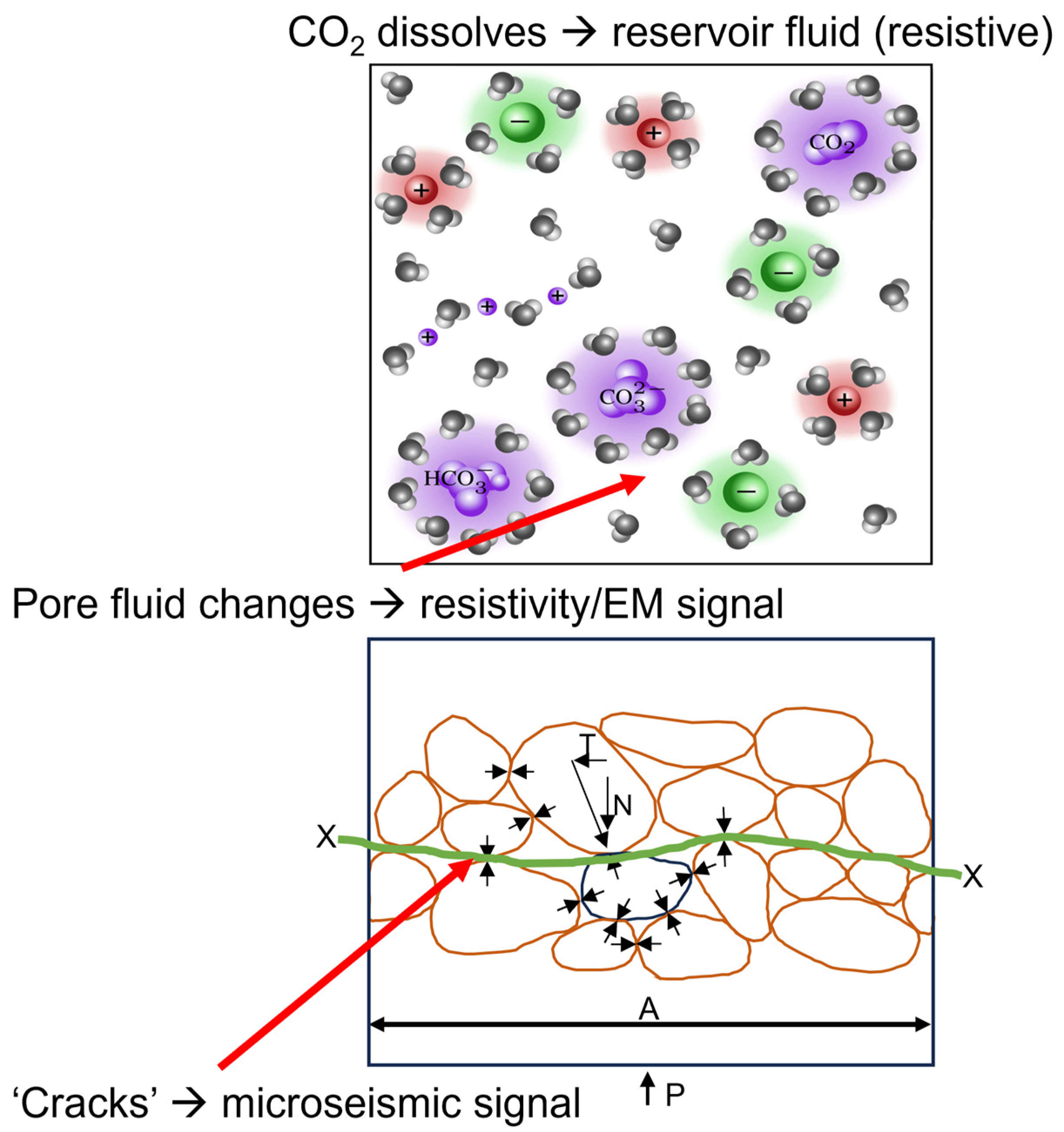
Figure 1 shows some models for the fluids in a CO
2 reservoir (top) [
13] and the structure in a hydrocarbon reservoir (bottom) [
14]. In the CO
2 injection case, the CO
2 combines with the water in the brine and builds larger molecules [
13] that are neutrally charged (colored purple in the figure). As a result, fewer electrons are available to provide current flow, and the reservoir is more resistive. In the figure on the bottom, a rock model made up of grains and pore space [
14] is considered. The pores are filled with fluid, and when strain/stress are impressed upon it, the brine fluid’s mobility and electron flow increase, causing a resistivity reduction. Once the pressure on the grain-to-grain contact increases, the reservoir seal breaks, generating a microseismic signal. Similar to the fluid model described above, any water saturation in the reservoir fluid contains free electrons. When the plume front moves through the reservoir, it exerts pressure on existing fluid (and even causes microseismic signals when the seal breaks). This pressure will cause the free electrons to flow and strong resistivity reduction right at the plume front, followed by the resistive plume. In the case of CCUS, this is caused by a fluid pressure wave due to the injection. Thus, CO
2 injection causes a resistive plume in a brine reservoir, and resistivity reduction at the edges can be observed.
Electromagnetic (EM) methods are sensitive to resistive contrasts [
15]; therefore, they are ideal for estimating the location and extent of an injected CO
2 plume. Multiple time-lapse surveys can be used to observe the change in resistivity because of the injection of CO
2 and its subsequent movement. Measurements taken before CO
2 injection can provide a baseline against which future changes can be evaluated. Time-lapse Controlled-Source ElectroMagnetic (CSEM) surveys combined with magnetotelluric (MT) surveys are a valuable tool for monitoring injected industrial CO
2 as a part of CCUS processes. Even if the changes caused by the CO
2 are small, it should be confirmed with confidence that changes seen in the data are only because of the movement of the CO
2 and not noise sources such as naturally occurring electric fields, surveying mistakes, or local anthropogenic features.
When surface CSEM measurements are tied to 3D anisotropic models derived from the available logs and lithology from the area under investigation as part of an initial 3D feasibility workflow, baseline measurements can be verified within the context of the borehole information, representing a significant risk reduction.
An initial 3D feasibility modeling workflow includes field noise measurements to determine the noise level and, thus, the best experimental source-sensor geometry and acquisition parameters based on the expected fluid substitution models. Careful instrument calibration and verification of all acquisition parameters are essential for data acquisition. Concurrent with the acquisition, near-real-time quality assurance and control (QA/QC) are carried out. The feedback verification loop results positively influence the acquisition’s data quality by optimizing operation times/equipment moves.
This process defines the proper length of acquisition time and consequently yields good data quality that can then be used for unsupervised inversion. The only influencing components in the inversion are the data weights derived from the repeated measurements (stacking weights). CSEM and MT data acquisition can benefit from this process and achieve high sensitivities for deep reservoir targets.
Achieving log scale resolution from surface measurements is a significant breakthrough; thus, baseline measurements can be verified before acquiring the monitoring measurements. Based on the results, the time-lapse (monitoring) survey can be further fine-tuned to reduce the success risk by taking the data integration from a subjective interpretation to an automated mere data display. This step requires hardware control and operation parameters (frequently repeated calibration) to obtain higher accuracy than is normal for exploration purposes.
Applying EM data acquisition systems to rare minerals exploration has demonstrated the need for careful hardware design to achieve high amplifier fidelity. This results in the ability to record subsurface responses requiring a high dynamic range from high resistivity contrast. Lithium prospecting represents such a challenge as lithium has a resistivity comparable to seawater at several hundred meters’ depth. Electric and EM methods are suited for lithium prospecting due to their sensitivity to very low electrical resistivity (typically 0.1 to 0.5 ohm-m) associated with the brine-saturated multilayers present and with a frequency/time window. These methods require specific equipment characteristics (as used for time domain CSEM) with instantaneous dynamic range.
In the next sections, we present CCUS, geothermal, EOR, and critical mineral case histories using EM methods.
2. Case Histories
The initial case study exemplifies the application of a feasibility workflow to a baseline data set obtained through the long-offset transient electromagnetic method (LOTEM) [
16]. This method is a variation of the CSEM method, which was integrated with the MT method for a time-lapse survey in Center, North Dakota, USA, as a part of a CCUS project. This example describes rigorous quality control and assessment methods, including noise removal and data validation with 1D and 3D inversion to tie results to borehole logs. The results are an accurate and representative CSEM data set and information that stakeholders can use to inform future time-lapse survey costs and designs.
The second case history is a geothermal example from Saudi Arabia focusing on exploration. The EOR case history examples include a modeling and feasibility study and a field test from the Middle East.
Finally, lithium exploration’s critical minerals case histories in Argentina and Saudi Arabia are described. The first is from an area where lithium reserves are known, and the second is from an area where they are suspected based on our findings.
All case studies were conducted utilizing the same equipment for CSEM and MT surveys. The equipment was designed for monitoring purposes, ensuring high repeatability, long-term stability, and minimum influence of system bandwidth limitations on signal bandwidth. The transmitter used was either a 100 (EOR example) or 150 (CCUS and Saudi Arabia examples) kVA transmitter, as described in [
17]. The array acquisition system for the CSEM (LOTEM) and MT configurations is described in [
18]. For more information on the system architecture and survey design, see [
15]. Furthermore, additional references for data processing, data interpretation, and inversion activities considered in the case studies can be found in
Appendix A.
2.1. Monitoring of CO2 in a Saline Reservoir in North Dakota, USA
Measurements taken before CO2 injection can provide a baseline against which future changes can be evaluated. Multiple time-lapse surveys can be used to observe the change in resistivity because of the injection of CO2 and subsequent movement.
Baseline EM methods were applied to assess their performance in CO
2 monitoring in the lower Permian Broom Creek and Cambrian and lower Ordovician Deadwood formations in the Williston Basin near Center, North Dakota, USA. Approximately 4 million metric tons of CO
2 annually are expected to be injected into the Broom Creek and Deadwood formations at depths of approximately 1450 and 2835 m and average thicknesses of 70 m and 85 m, respectively.
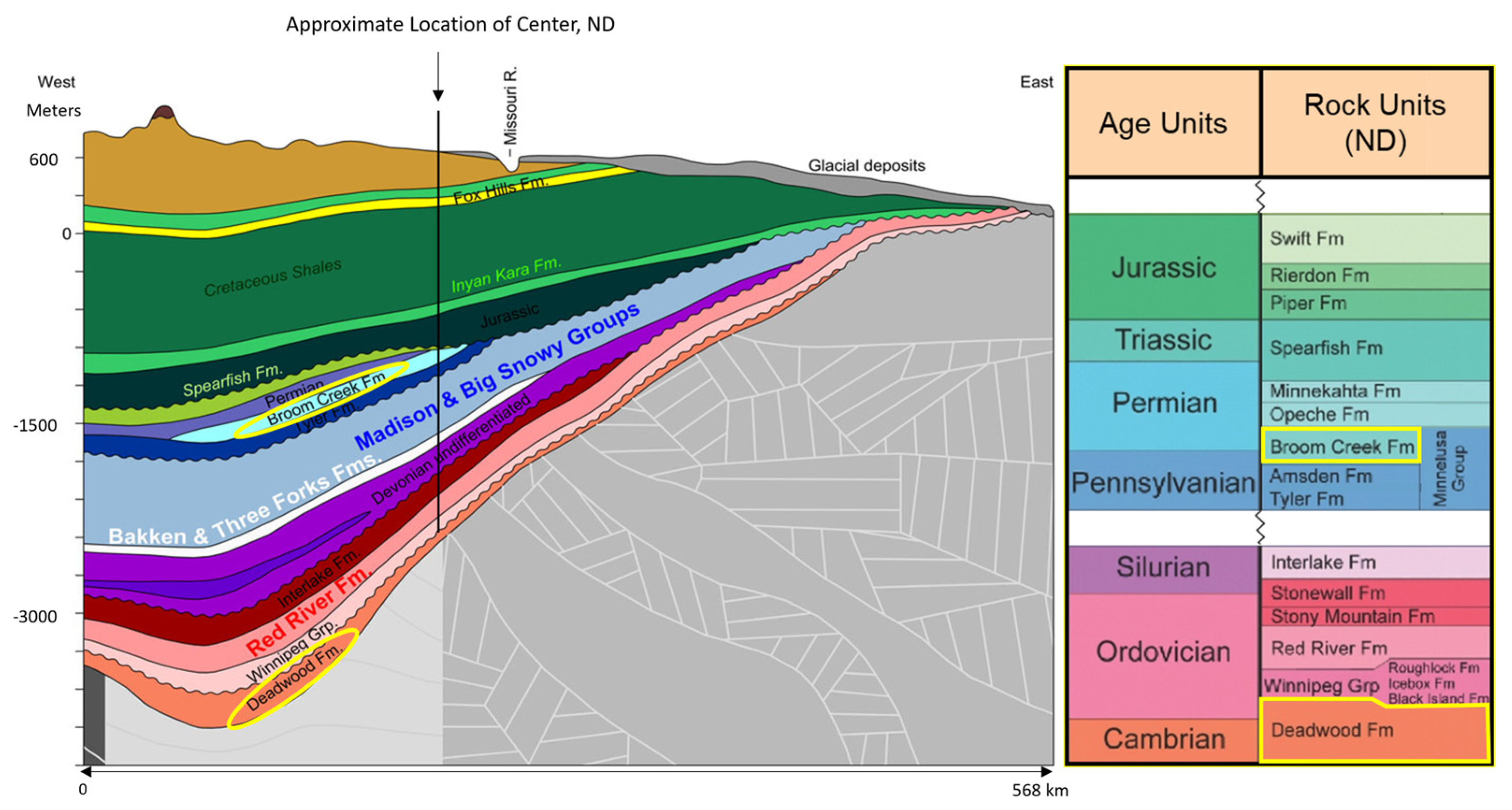
Figure 2 shows a simplified cross-section of North Dakota with the studied reservoirs (yellow ellipses) and a simplified stratigraphic column, including the formations overlying and underlying the studied reservoirs. The vertical black line represents the approximated location of the studied area.
The major Broom Creek lithofacies are eolian sandstone, nearshore marine sandstone, marine carbonate, and anhydrite. The Broom Creek Formation in the study area can be divided into upper, middle, and lower sandstone-dominated intervals, with an average porosity of 23% and median permeability of 100 mD. Mudstones, siltstones, and interbedded evaporites of the undifferentiated middle Permian Opeche and upper Permian–Triassic Spearfish formations unconformably overlie the Broom Creek Formation. Mudstones and siltstones of the lower Jurassic lower Piper Formation (Picard Member and lower) overlie the Opeche–Spearfish formations. The lower Piper and Opeche–Spearfish formations serve as the primary confining zone for the CO
2 storage reservoir, with an average thickness of 47 m. The upper Pennsylvanian Amsden Formation (dolostone, limestone, and anhydrite) unconformably underlies the Broom Creek Formation and serves as the lower confining zone, with an average thickness of 82 m [
19]. The base of the Broom Creek Formation is approximately 1500 m above the Precambrian basement.
The Deadwood Formation unconformably overlies the Precambrian of the Williston Basin and consists of siliciclastics, carbonates, and evaporites. The Deadwood can be divided into six members, A–F [
20]. The earliest Member A is Cambrian, composed of alluvially deposited conglomerates and sandstones. Member B consists of glauconitic shallow marine sandstones and siltstones. Members C–F consist of a lower Ordovician succession of three regressive–transgressive sequences containing sandstones, siltstones, mudstones, and carbonates. Members A–E are present in the study area. The Winnipeg Group unconformably overlies the Deadwood and consists of three formations: Black Island, Icebox, and Roughlock. The Black Island Formation is a mixture of sandstone and shale deposited in a fluvial–deltaic to shallow marine environment [
21]. The Icebox Formation conformably overlies the Black Island Formation. The Icebox is a marine shale that serves as the primary upper confining zone, with an average thickness of 36 m. The Roughlock is a calcareous shale to argillaceous limestone. The continuous shales of the Deadwood Formation B member serve as the lower confining zone, with an average thickness of 10 m. In addition to the Icebox Formation, there are 174 m of impermeable rock formations between the Black Island Formation and the next overlying porous zone, the Red River Formation [
19].
2.1.1. CSEM Feasibility Study
Injection of supercritical CO
2 into brine-filled reservoir rocks reduces the electrical conductivity and potentially produces a 4D anomaly that can be measured from the surface. We selected the CSEM method for CO
2 monitoring because it showed the strongest coupling to resistive and conductive formations [
22,
23]. A feasibility study was performed to determine the effectiveness of CSEM monitoring CO
2 injected into the Broom Creek and Deadwood formations [
24]. Although the ultimate proof will be the three-dimensional time-lapse image from potential repeat surveys, the feasibility study’s prediction was verified with the initial field data by comparing the model derived from the well logs with inversion results for the one-, two- and three-dimensional EM methods used in the project plus the three-dimensional anisotropic model from fitting the measurements of all CSEM components.
The goal of the 3D modeling [
25] was to estimate the expected surface EM field response level caused by an increase in CO
2 saturation and determine whether signals of that magnitude could be detected in the field in the presence of observed noise levels. Moreover, the feasibility study defined survey parameters, such as station spacing along survey lines, to maximize signal levels from target formations.
Integrating surface and borehole data is an essential requirement derived from 3D modeling. Data integration is achieved by measuring between surface and borehole, calibrating the information with conventional well logs, and considering resistivity anisotropy [
23]. This process reduces the risk of imaging false anomalies [
26,
27,
28,
29]. Hence, combining advances in acquisition hardware, imaging methods, 3D modeling, and workflow to integrate surface models with borehole measurements in a CO
2-monitoring scenario is paramount. High measurement accuracy and overall repeatability (better than 0.5%) are required in this scenario [
15]. This includes everything from instruments, operations, location repeatability, and environmental issues (atmospheric, cultural, and geologic noise). The target reservoir signal band must be well within the center of the entire system signal band to avoid deconvolution of potential system responses [
22].
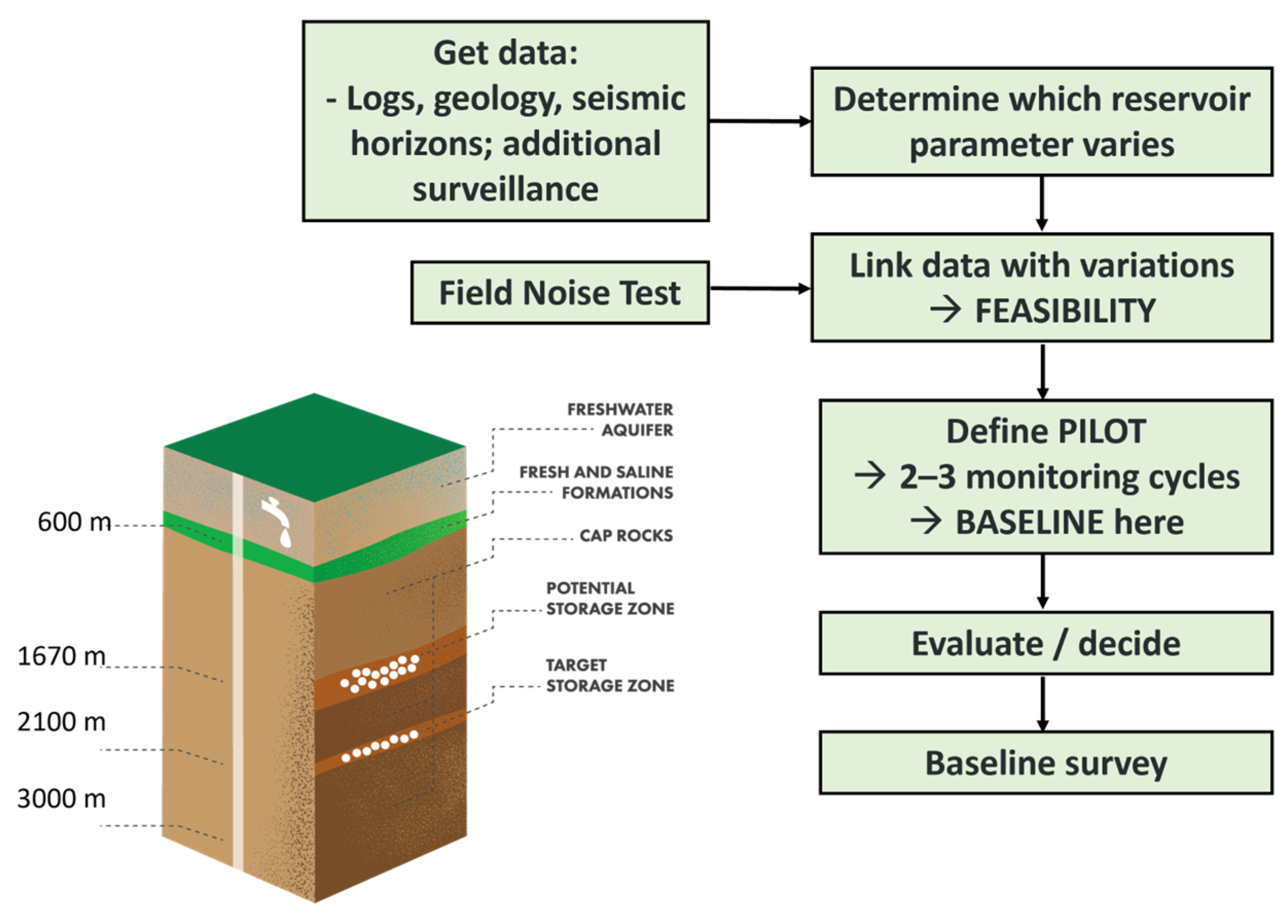
Figure 3 shows the CSEM feasibility workflow. The workflow’s input data are seismic horizons from two 3D seismic data sets and well logs from the four wells (A, B, C, and D) in the study area. Borehole resistivity logs are considered ground truth. Using an equivalencing process [
22,
30] and 3D modeling based on physics, we built a 31-layer equivalent model (3D anisotropic) that honors the lithological boundary and the log [
31].
Rock physics is an essential element of the feasibility workflow, which provides the means to connect rock properties and fluid saturation determined from geology or petrophysics with measurements from geophysics. Rock physics can be used to predict how changes to rock properties and fluid saturation will affect the geophysical measurements and, thus, the feasibility of using geophysics to monitor the storage and sequestration of CO2.
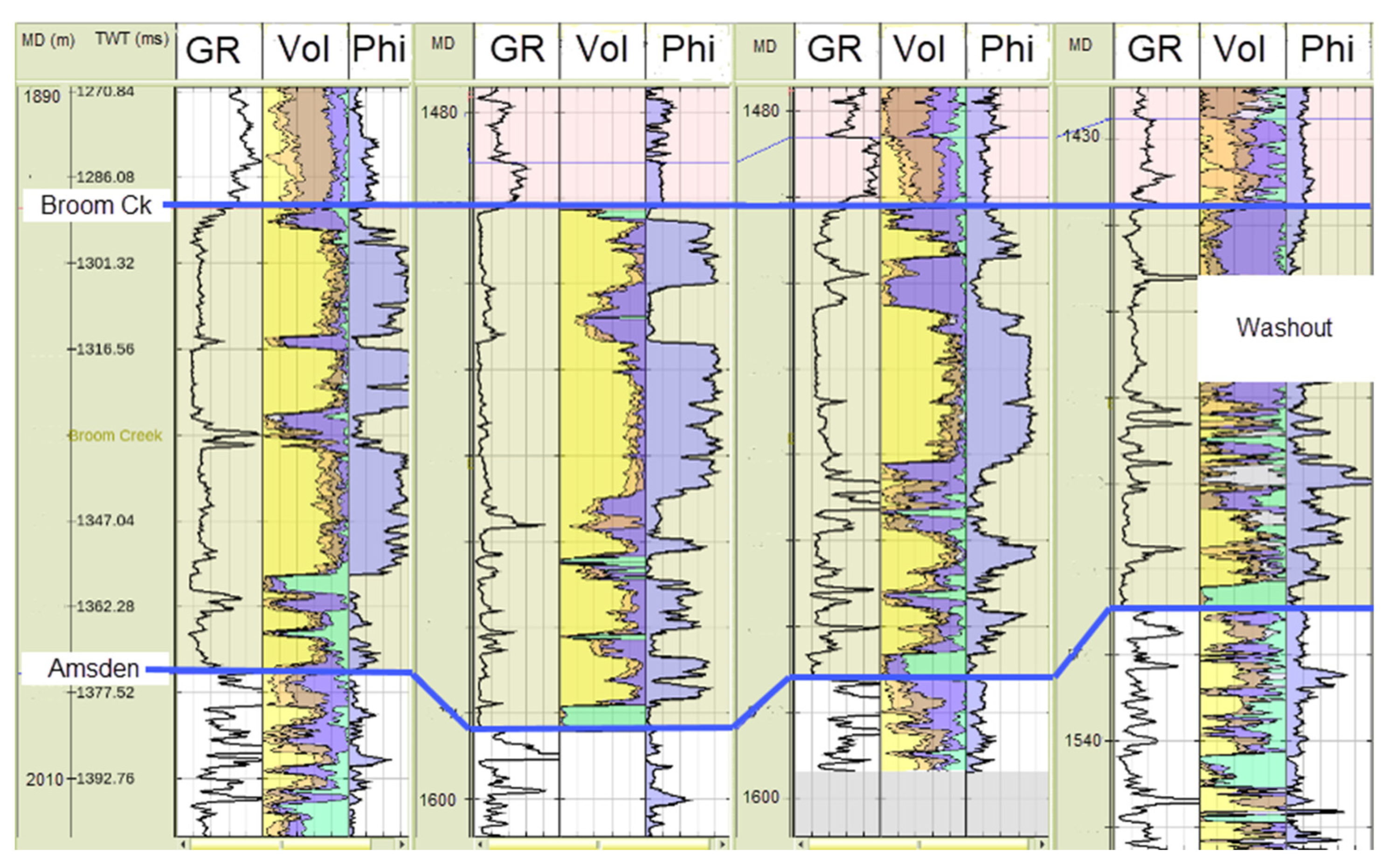
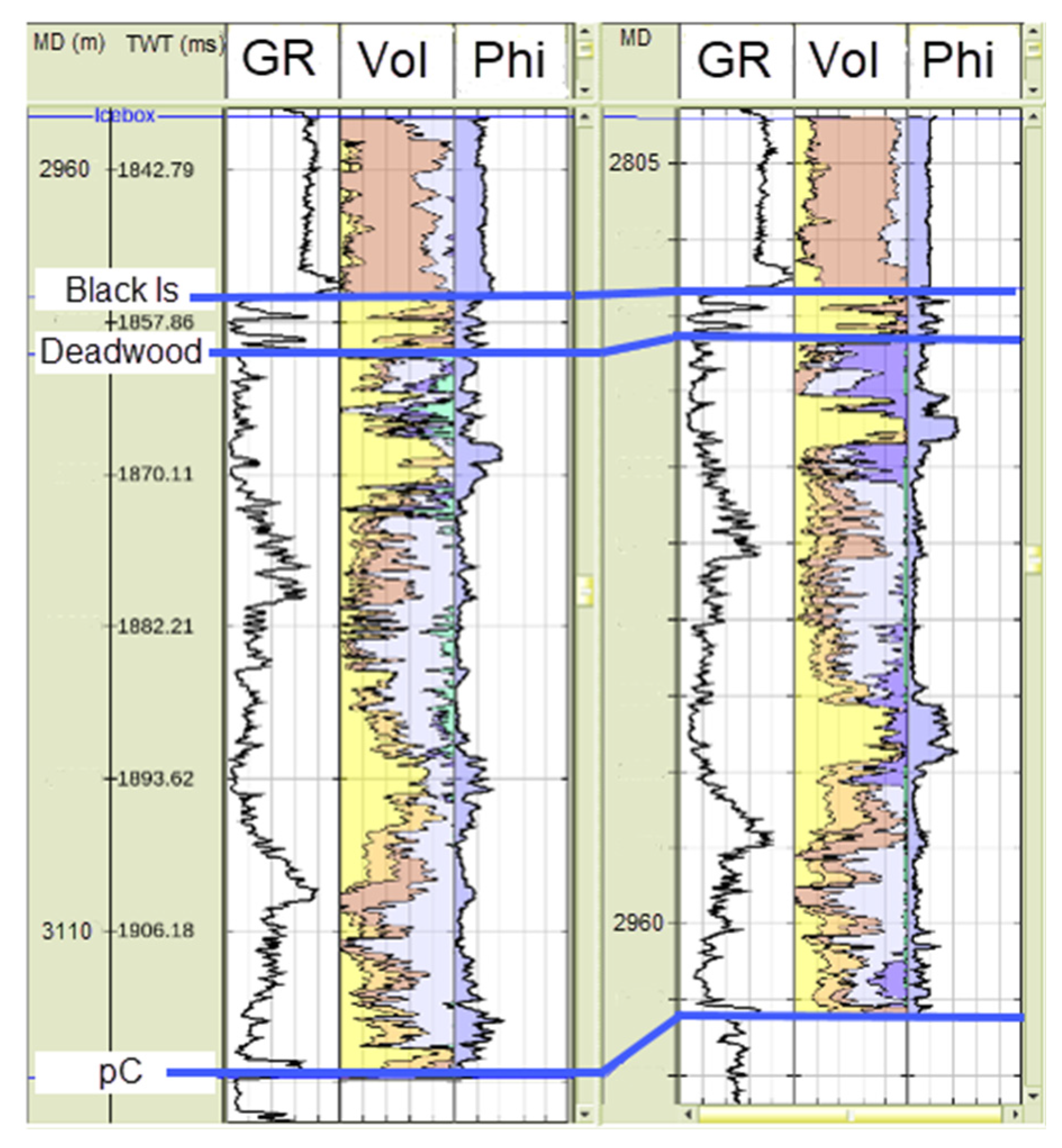
The geological data used in the rock physics analysis consist of regional geology, core descriptions from whole cores and thin sections, and core plug analysis results, including X-ray diffraction (XRD), X-ray fluorescence (XRF), and measurements of porosity, permeability, and grain density. Petrophysical data were corrected for tool and borehole effects and checked for consistency between wells. The volumes of the dominant minerals were used to determine the rock properties used in rock physics modeling. Lithology volume logs in the Broom Creek and Deadwood formations at each well were generated from the well logs using the TechLog Quanti.Elan module. The normalized solid volume results are shown in
Figure 4 and
Figure 5. The results were quality-controlled, comparing the predicted volume fractions and porosities with the weight fractions from core XRD and core porosities.
The results show that the Broom Creek Formation’s dominant lithologies are quartz, dolomite, and anhydrite. The Deadwood Formation’s dominant lithologies are quartz and carbonate, with smaller volumes of clay and feldspar.
The lithology volume logs were used to calculate density porosity and composite rock grain elastic properties for rock physics analysis. Porosity logs were used to model rock properties and fluid substitution. The porosity logs should be consistent with core measurements and geologically consistent between wells. Density porosity or phid [
32] was calculated from the density log using the lithology volume logs and formation brine densities from the Broom Creek and Deadwood formations.
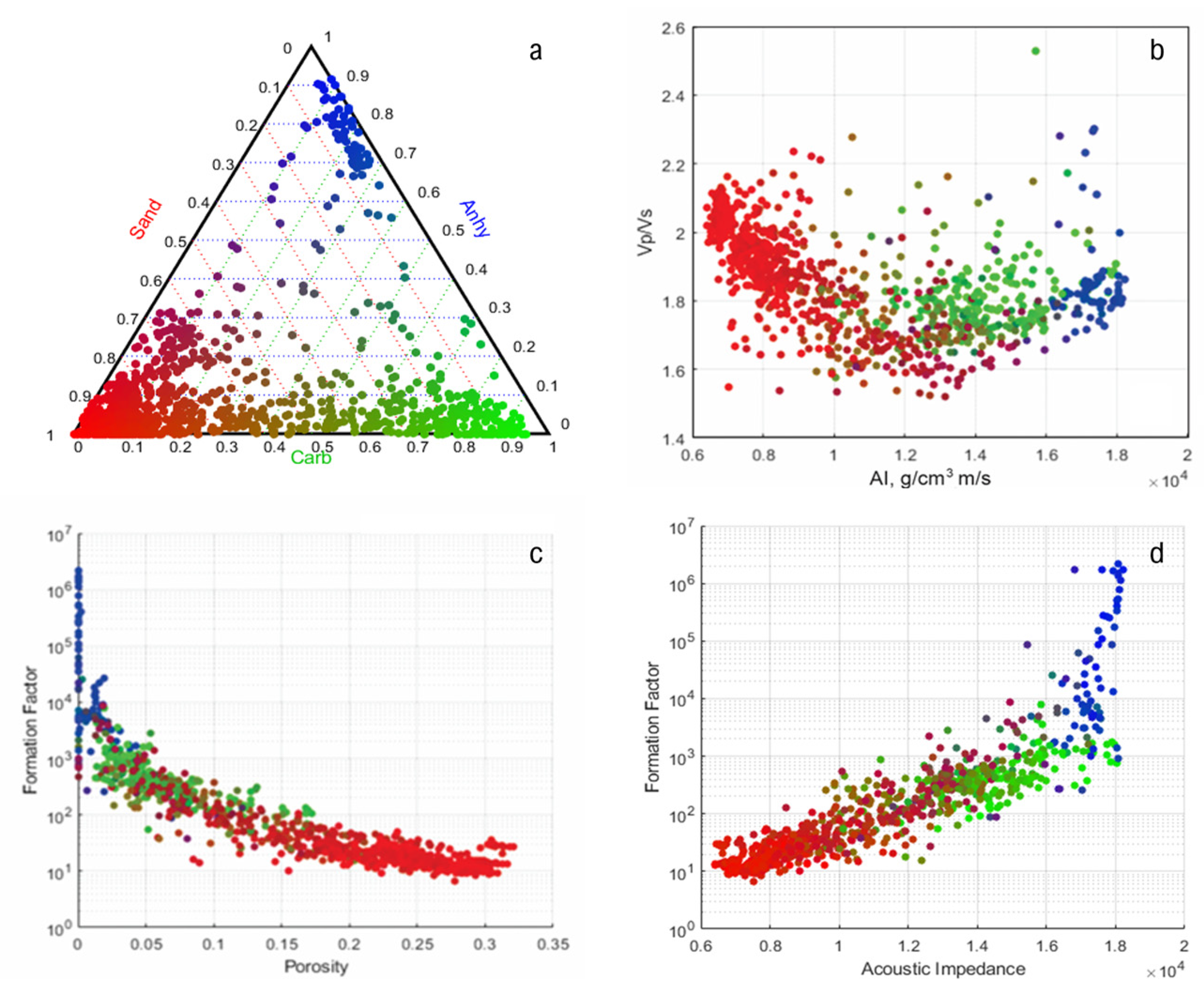
The crossplot analysis of Broom Creek (
Figure 6) based on wells A and C shows a complex formation dominated by a mixture of sand, dolomite, and anhydrite. The three-mineral mixture allows us to use a ternary plot to describe mineral composition. The sample points can be colored using a blend of red (sand), green (carbonate), and blue (anhydrite) in proportion to their rock compositions (
Figure 6a). For crossplot analysis, sand is defined as the sum of quartz and feldspar, and carbonate as the sum of calcite and dolomite. The ternary plot and crossplot are connected by applying the color blends as the z-values in the crossplot, creating an integrated plot with five dimensions of information. The P-wave velocity/S-wave velocity (Vp/Vs) ratio vs. acoustic impedance (AI) results in
Figure 6b indicate that sand has a low AI and high Vp/Vs ratio. In contrast, carbonates have a higher AI and lower Vp/Vs ratio. Anhydrite has the highest AI.
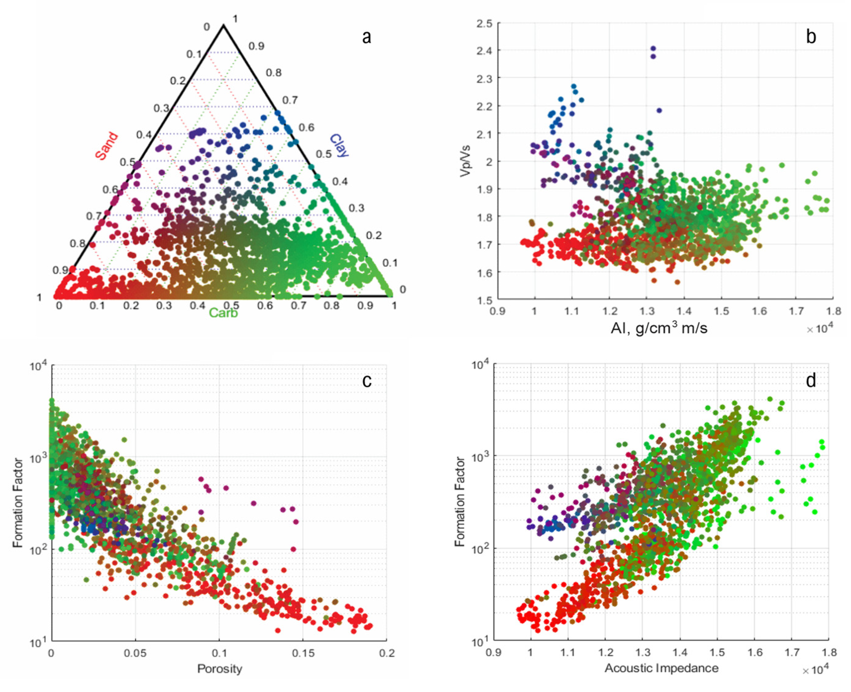
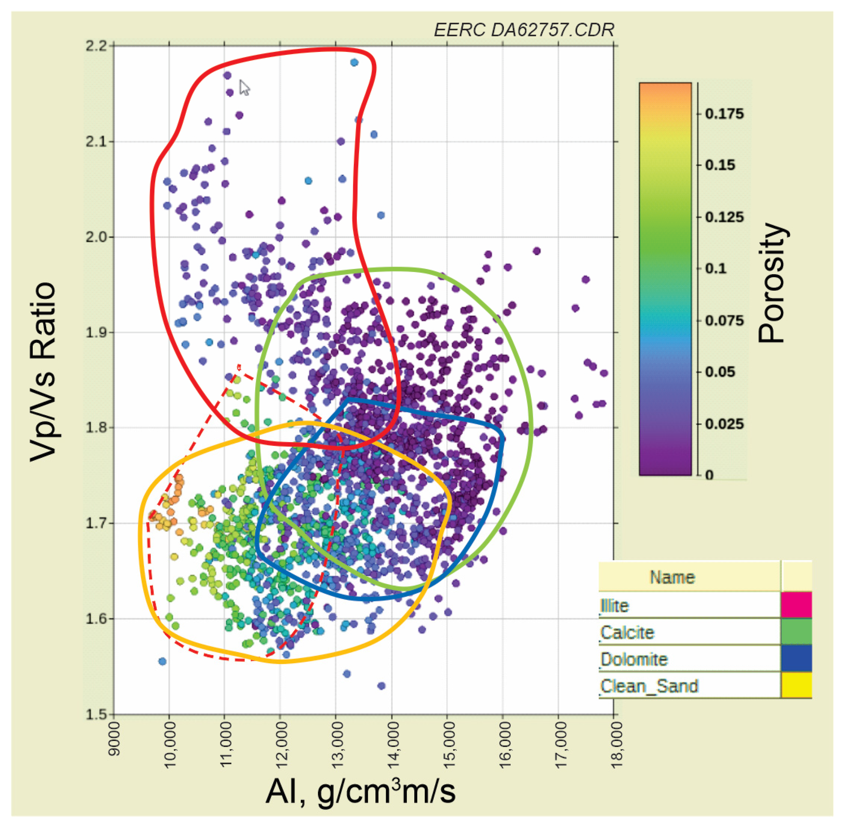
The B and D wells were used for the crossplot analysis of the Deadwood Formation (
Figure 7). The Deadwood Formation is a complex formation dominated by a mixture of sand (quartz + feldspar), carbonate (calcite + dolomite), and clay, which were used to create a ternary crossplot of mineral composition and rock physics properties. In the ternary plot (
Figure 7a), mineral proportions are colored by mixing red (sand), green (carbonate), and blue (clay) in proportion to their volumes. The color is used to color the ternary plot and the samples (z-axis) of the crossplot. The results in
Figure 7b indicate that sand is characterized by low AI and low Vp/Vs ratio, while the clays have a low AI and high Vp/Vs ratio. The carbonates have high AI and intermediate Vp/Vs ratios.
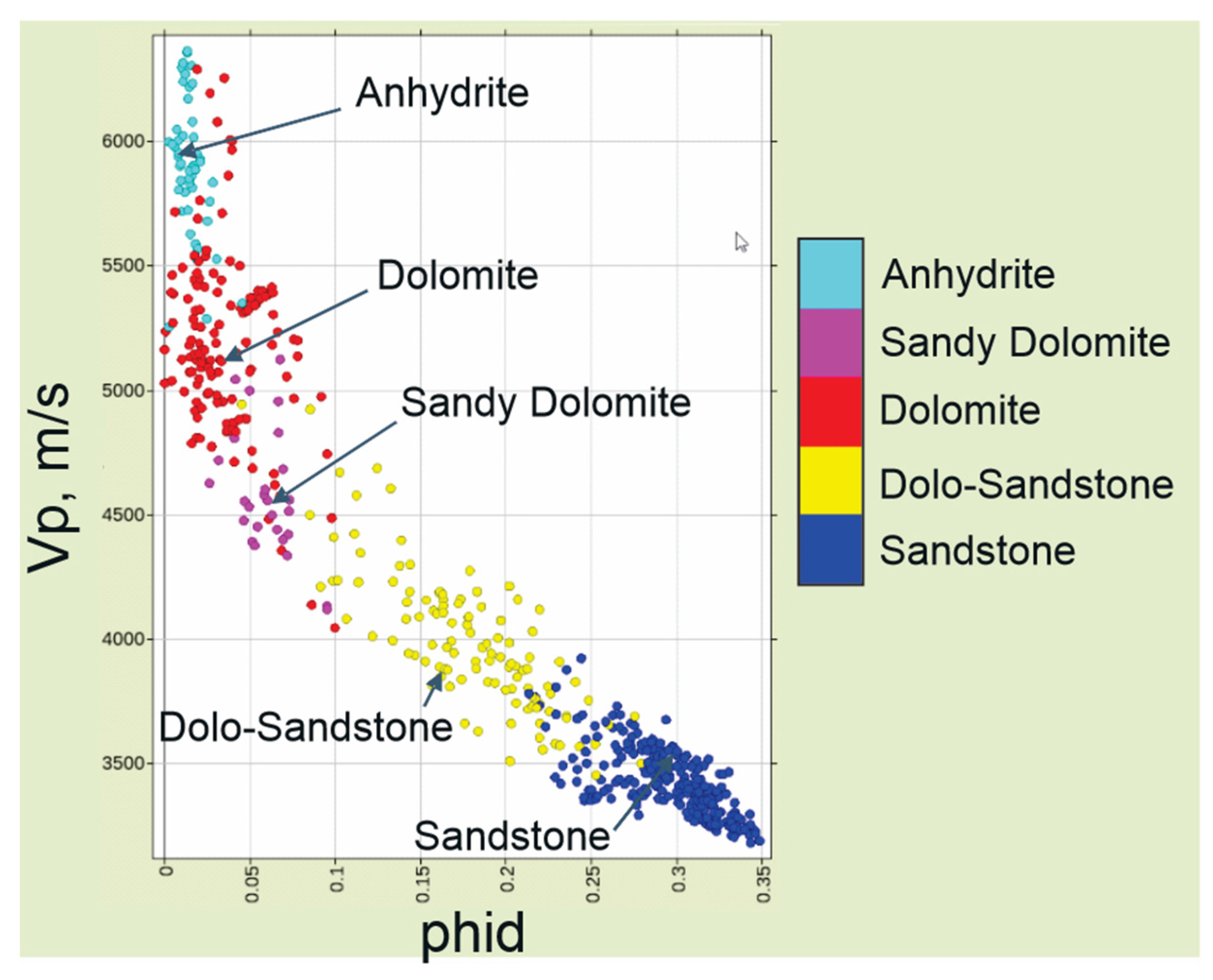
Variations in rock physics properties can be linked with changes in geologic facies. The changes in composition, porosity, sorting, and diagenesis change the formation’s elastic, density, and electrical properties. The geologic facies were found using the Heterogeneous Rock Analysis
® (HRA
®) module in Techlog
®. In Broom Creek, HRA was used to define five rock types. The inputs to the facies analysis included triple-combo (tool string designed to measure formation density, porosity, deep/intermediate/shallow resistivity, natural gamma, radiation, hole size, and fluid temperature) and NMR wireline logs. The facies were characterized based on core data, including thin sections, XRD, and XRF. The results of the facies relationship to rock physics properties are shown in the Vp vs. phid crossplot in
Figure 8. The sandstone facies have high porosity and Vp, and anhydrite have low porosity and high Vp.
The Deadwood–Black Island lithologies identified from Techlog Quanti.Elan inversion were used in a Vp/Vs vs. AI rock physics crossplot, as depicted in
Figure 9, to identify facies trends for rock physics analysis. The polygons were created by applying lithology cutoffs to the data and then creating polygons to group the points. The lithology cutoffs used for the crossplot are sand ≥ 0.64 and illite, calcite, and dolomite each ≥0.36 by volume. Density porosity > 0.1 was also identified. The polygons show that the high porosities are associated with sand and that calcite and dolomite overlap and could be merged to form carbonate facies.
Fluid Elastic Properties
The fluids in the pore space affect the rocks’ effective elastic and electrical properties. In general, liquids have higher density and bulk modulus than gases. Two fluids, brine, and CO2 are expected to be present in Broom Creek and Deadwood during sequestration. The brine in Broom Creek is assumed to have a salinity of 64,100 ppm NaCl equivalent based on a sample from the Broom Creek Formation in the C well.
The properties of CO
2 are dependent on the pressure and temperature of the reservoir. The Broom Creek Formation in the study area has a temperature and pore pressure of 58 °C and 17 MPa. When the temperature and pressure are above 31 °C and 7.3773 MPa, CO
2 is in a supercritical phase. In this state, CO
2 has a liquid’s density and a gas’s bulk modulus. The elastic properties in
Table 1 were calculated at Broom Creek reservoir conditions. Brine properties were calculated with the FLAG calculator [
33] built into RokDoc. The properties of dry CO
2 at reservoir conditions were calculated by the NIST CO
2 property calculator [
34].
A small amount of CO
2 will dissolve into the brine to produce a CO
2-saturated brine [
35]. Han and Sun [
36] measured the density and Vp of CO
2–water mixtures at typical reservoir temperatures and pressures. These authors produced empirical equations to predict the bulk modulus and density of CO
2-saturated brine. Their equations were used to approximate the properties of CO
2-saturated brine in the Broom Creek Formation. The CO
2-saturated brine has a saturation of 27.6 L/L at standard temperature and pressure conditions of 15.56 °C and 0.10133 MPa. The results are given in
Table 1. Alternative property estimates for CO
2-saturated brine can be found in the literature, including [
35,
37].
The Deadwood Formation in the study area has a temperature and pore pressure of 83 °C and 31.7 MPa. Any CO
2 injected into it will be supercritical. The bulk modulus and density of the fluids in the Deadwood pore space affect the effective elastic properties sensed by the seismic data. The elastic properties of the fluids at reservoir conditions are given in
Table 2. Based on the fluid properties, free CO
2 in the reservoir will reduce the effective density and Vp of the reservoir and, depending on the rock’s stiffness, may produce a contrast with the brine-filled reservoir. A small amount of CO
2 is expected to dissolve into the brine, with a maximum saturation of 17.3 L/L at standard conditions.
Fluid mixing of CO
2 and brine can vary between homogeneous and heterogeneous. In the reservoir, CO
2 and brine will mix at all scales, where the amount of mixing depends on reservoir properties [
38] and the engineering characteristics of the injection process [
39]. If the reservoir is in capillary equilibrium, the brine and CO
2 saturation distribution will be controlled by capillary pressure curves associated with various geologic facies. Since capillary pressure is significantly influenced by permeability, variation of reservoir permeability has a significant role in saturation distribution [
38]. Adams et al. [
40] and Barajas-Olalde et al. [
41] published in-depth rock physics studies of the Broom Creek and Deadwood formations for seismic CO
2 monitoring in the study area.
Electromagnetic Properties
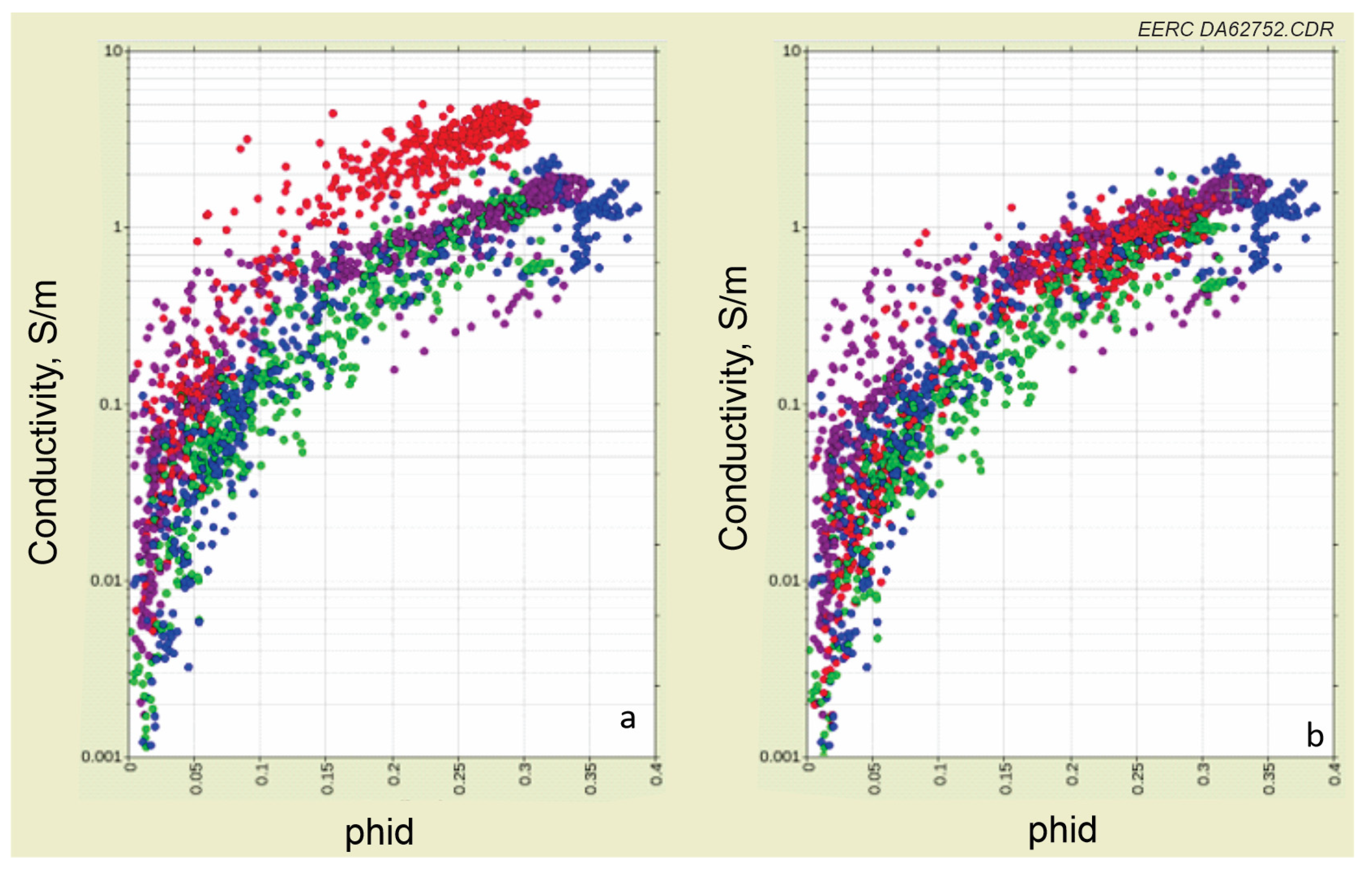
The conductivity of the minerals and fluids in the formation and the conductivity of the drilling mud affect electrical resistivity or conductivity logs. In the Broom Creek Formation, brine resistivities were measured in the A, B, and C wells. Fluid replacement modeling using Archie’s equation [
42] was used to normalize the electrical conductivity and formation factors of the A, C, and D wells to the B well. The original electrical conductivity is shown in
Figure 10a, and the final conductivity after substitution is shown in
Figure 10b. The electrical conductivities were more consistent after fluid replacement.
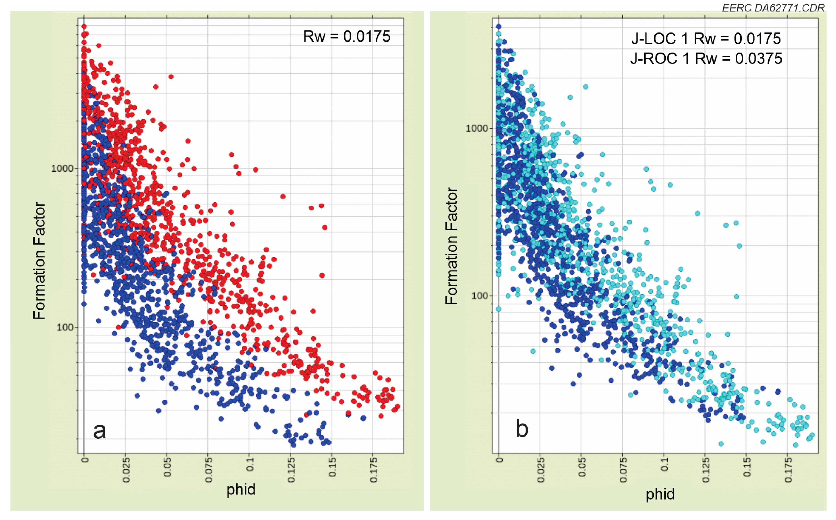
Deadwood brine salinity was measured only in the B well. Initially, the measurement was used for both wells (see
Figure 11a). The sample distributions for the B and D wells were inconsistent. A consistent result was obtained after adjusting the D fluid resistivity (Rw = 0.0375 ohm-m), as shown in
Figure 11b. The mud filtrate’s resistivity (Rm) in the D well was 0.0329 ohm-m at 83 °C, which suggests that mud filtrate is a significant factor in the D resistivity readings.
Rock Electrical Properties
Most common rock-forming minerals, except for clay, are insulators at the frequencies used in geophysics. Under these conditions, the electrical conductivity of the formation is determined by the electrical conductivity of the brine and the porosity/permeability of the rock [
43]. Formation factor [
42] provides a way of normalizing resistivity or conductivity logs for the influence of changes in brine resistivity between wells.
Ternary crossplots were also used to examine the relationship between the Broom Creek and Deadwood Formations’ porosity, lithology, and formation factor, as shown in
Figure 6c and
Figure 7c, respectively. In
Figure 6c, the lowest formation factors (10–100) of the Broom Creek Formation are associated with high-porosity (>0.15) sand, while carbonate is low-to-medium porosity (0.02–0.15) and has intermediate formation factors (100–2000). Anhydrite is associated with the lowest porosity (<0.05) and the highest formation factors (>2000). For the Deadwood Formation (
Figure 7c), the distribution is continuous where the lowest formation factors (10–30) are associated with high-porosity (>0.15) sand, the highest formation factors (>200) are associated with low-porosity carbonate (<0.05), and clay is related to low porosity (<0.07) and intermediate formation factors (100–200).
The electrical and elastic properties of a rock have no common fundamental physics properties. However, as shown for Broom Creek in
Figure 6d and Deadwood in
Figure 7d when cross-plotted, they show significant correlation. The cleanest sands are associated with low acoustic impedance and formation factor; increasing the volume of carbonate causes both properties to increase. The connection creating the correlation is an arrangement of the minerals in the rock. Correlations like this suggest that electromagnetic and seismic methods provide complementary information about the reservoir.
Fluid Electrical Properties
The Broom Creek electrical resistivity in
Table 1 was determined from Schlumberger well log interpretation tables [
44]. Supercritical CO
2 is assumed to be an insulator. The authors of [
45] cite a value of 1 × 10
−8 S/m in their review paper. The CO
2-saturated brine in the Broom Creek Formation is expected to have a saturation of 27.6 L/L CO
2 at standard conditions. Using the equations given by [
13], CO
2-saturated brine is expected to have 0.9 of the conductivity of the original brine.
The brine salinity 256,000 ppm NaCl equivalent in the Deadwood Formation was determined from a sample acquired in the B well. The D brine was assumed to have the same salinity. Supercritical CO
2 is assumed to be an insulator. A small volume of CO
2 can enter into a solution with brine. In the Deadwood Formation, the saturation is expected to be 17.3 L/L CO
2 at standard conditions. The electrical conductivities of the three fluid phases are given in
Table 2. CO
2-saturated brine had an electrical conductivity of 0.93 of the brine. Given various CO
2 saturation levels, many 3D models were calculated for the feasibility study.
Table 1.
Broom Creek Formation elastic and electric fluid properties.
Table 1.
Broom Creek Formation elastic and electric fluid properties.
| Fluid | T
(°C) | P
(MPa) | Density (kg/m3) | Vp
(m/s) | K
(GPa) | σ
(S/m) | Boerner Coefficient | Elastic Reference | Electrical Reference |
|---|
| Brine | 58 | 17 | 1035 | 1642 | 2.791 | 15.38 | NA * | [33] 1 | [44] |
| CO2 | 58 | 17 | 681 | 365 | 0.091 | 0 | NA | [34] 2 | Assumed |
| CO2-Saturated Brine | 58 | 17 | 1043 | 1637 | 2.797 | 13.79 | 0.8963 | [36] | [13] |
Table 2.
Deadwood Formation elastic and electrical fluid properties.
Table 2.
Deadwood Formation elastic and electrical fluid properties.
| Fluid | T
(°C) | P
(MPa) | Density (kg/m3) | Vp
(m/s) | K
(GPa) | σ
(S/m) | Boerner Coefficient | Elastic Reference | Electrical Reference |
|---|
| Brine | 83 | 31.7 | 1168 | 1816 | 3.852 | 57.14 | NA * | [33] 1 | [44] |
| CO2 | 83 | 31.7 | 750 | 488 | 0.179 | 0 | NA | [34] 2 | Assumed |
| CO2-Saturated Brine | 83 | 31.7 | 1176 | 1811 | 2.86 | 52.98 | 0.9272 | [36] | [13] |
CSEM 3D Modeling
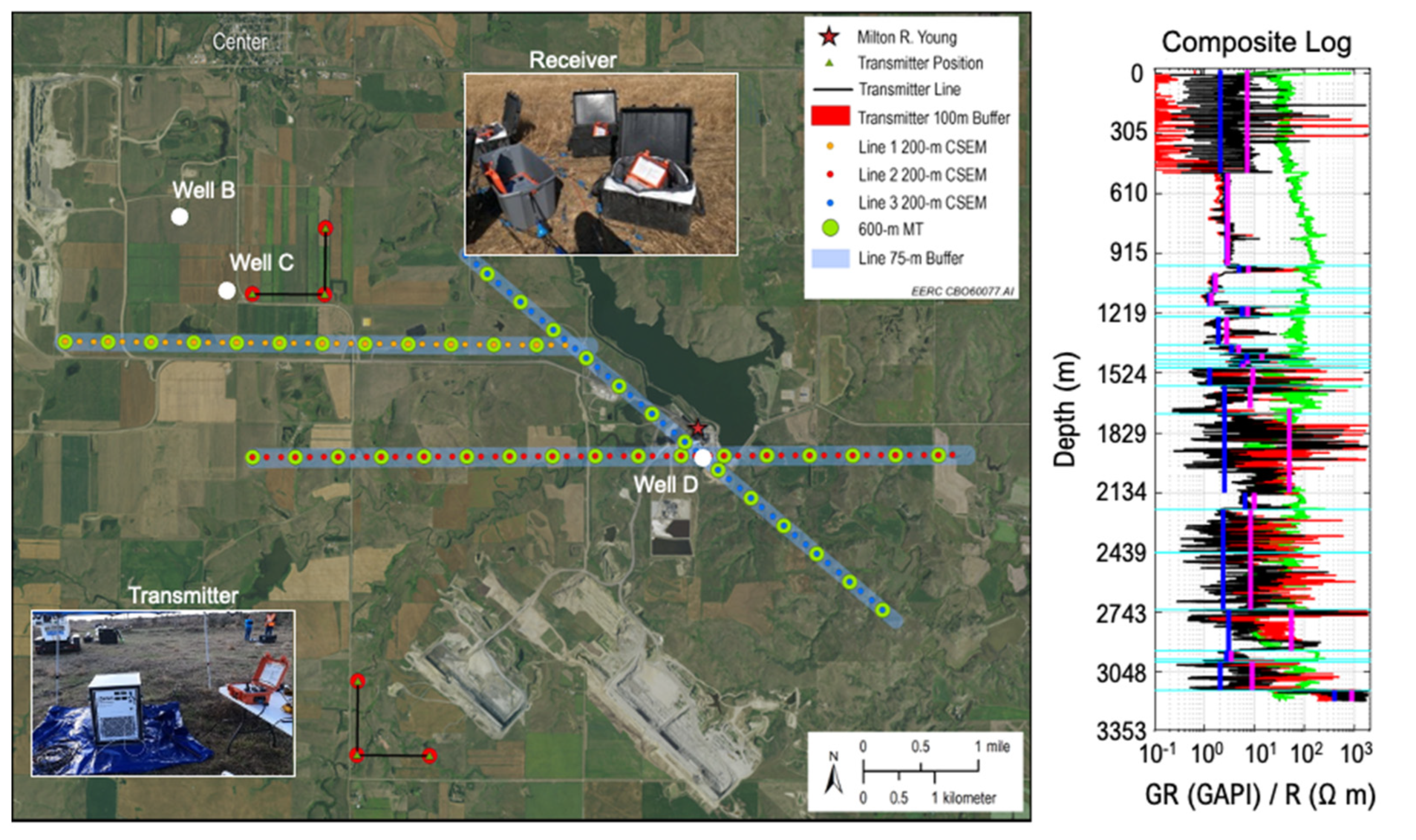
The CSEM setup includes a transmitter and receiver moved along profile lines, as shown in
Figure 12. The survey layout consists of three lines of receivers and two separate CSEM transmitter sources to the north and south of these lines. We chose two transmitters to see and account for larger directional structural changes and anisotropy effects. More details on the hardware can be found in Strack et al. [
15]. Each transmitter had two dipoles in perpendicular directions to account for local anisotropy variations. The log was scaled to 32 layers with anisotropic resistivities shown superimposed on the log on the right of
Figure 12. The upscaling was verified with 3D modeling within 1%, and seismic and lithologic boundaries were maintained. The upscaled log represents the ground truth for CSEM based on the well logs.
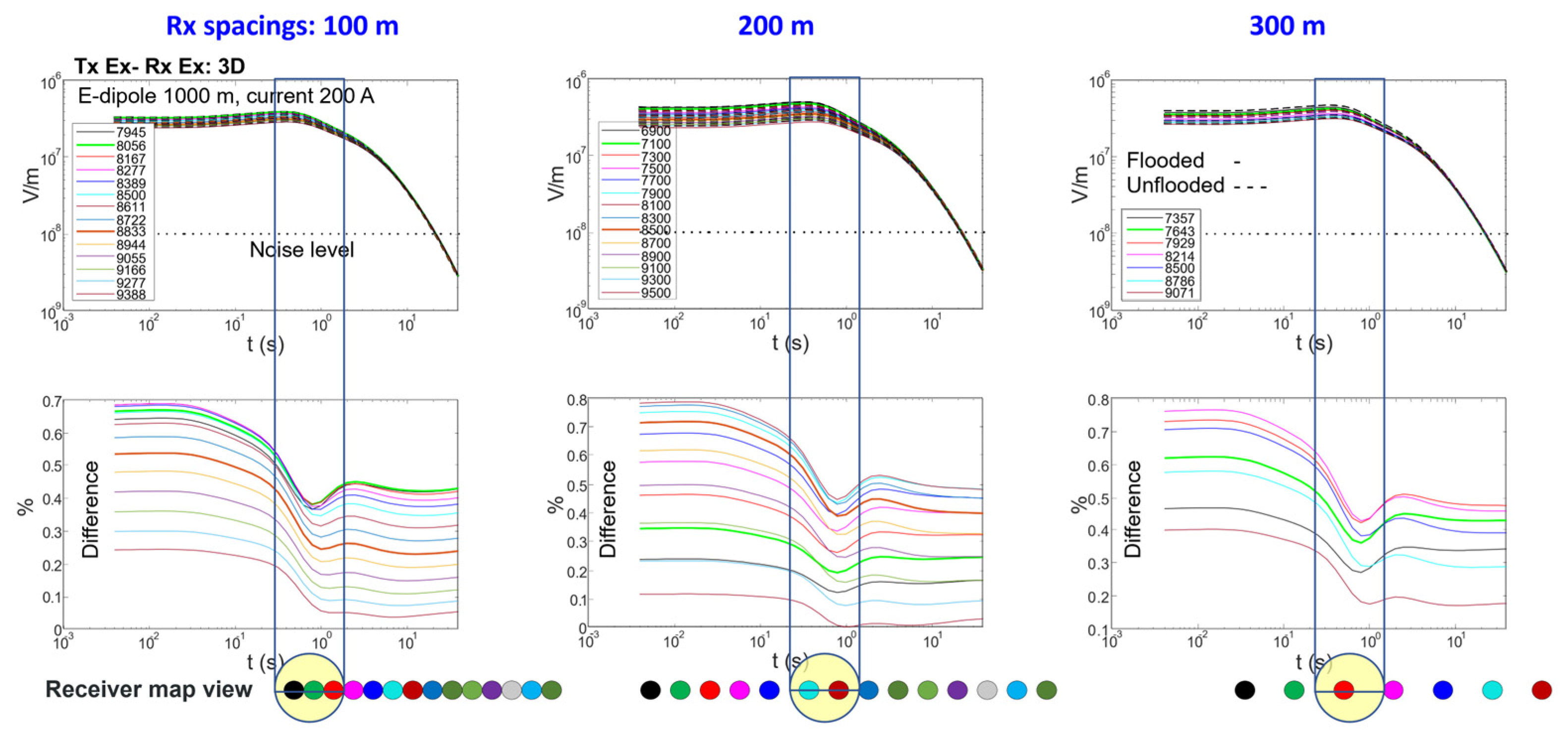
For the 3D modeling, one transmitter and fourteen receivers along the three-receiver lines were used to build various 3D modeling tests. In the field, 13 receivers were moved along the profile lines. The receivers were at the injection well and represent the most distant receivers from Transmitter Location 1 (north location in the study area) and serve as a reference. All electromagnetic field responses and the time changes were modeled. An exemplary display is shown in
Figure 13 for the Broom Creek Formation. These models were also used to estimate the optimum parameter range. Here, the results are displayed in the context of defining the optimum station spacing by displaying the 100 m, 200 m, and 300 m site spacing. The curve colors correspond to the site locations shown at the bottom of the figure, along with the chosen injection plume radius. Note that the plume radius can be seen on all curves.
Furthermore, the curves can be interpolated from the left to the right. The largest total amplitude in the electric field values can be seen for the 200 m spacing, which is why this was chosen for the survey. All other components behaved similarly. The benchmark models covering most field scenarios were based on petrophysical analysis. Then, the equipment/sensor choice was added to the 3D modeling results. The result is a set of models including the expected anomaly within the measurable time window.
Twenty-one months of CO
2 injection in the Broom Creek Formation was simulated using a 60% average CO
2 saturation and an injection radius of 500 m. The simulation showed that 15–18 months of injection produced a strong anomaly. Next, an injection radius of 150 m was used, and the required receiver spacing was estimated.
Figure 13 depicts the 3D modeling results for the Broom Creek Formation for Ex (Ey and dBz/dt are not shown here). The reference noise from the noise test is shown at each component (horizontal dotted line). The response of all the components is above the noise level. The curve variations between the three spacings are smooth; therefore, the CO
2 anomaly can be reconstructed for 100 m, 200 m, and 300 m receiver spacings.
As the Deadwood Formation has lower porosity and is significantly deeper than the Broom Creek Formation, a conservative 30% CO2 saturation after injection (representing a 150 m flood zone radius) was considered. The responses and differences corresponding to reservoir conditions before and after CO2 injection were between 1% and 5% for a 1D model and below 1% for 3D models. Based on these results, monitoring injected CO2 in the Deadwood Formation under the assumed field and survey parameters will be challenging, and novel anomaly-enhancing methods will be needed.
Field Noise Test
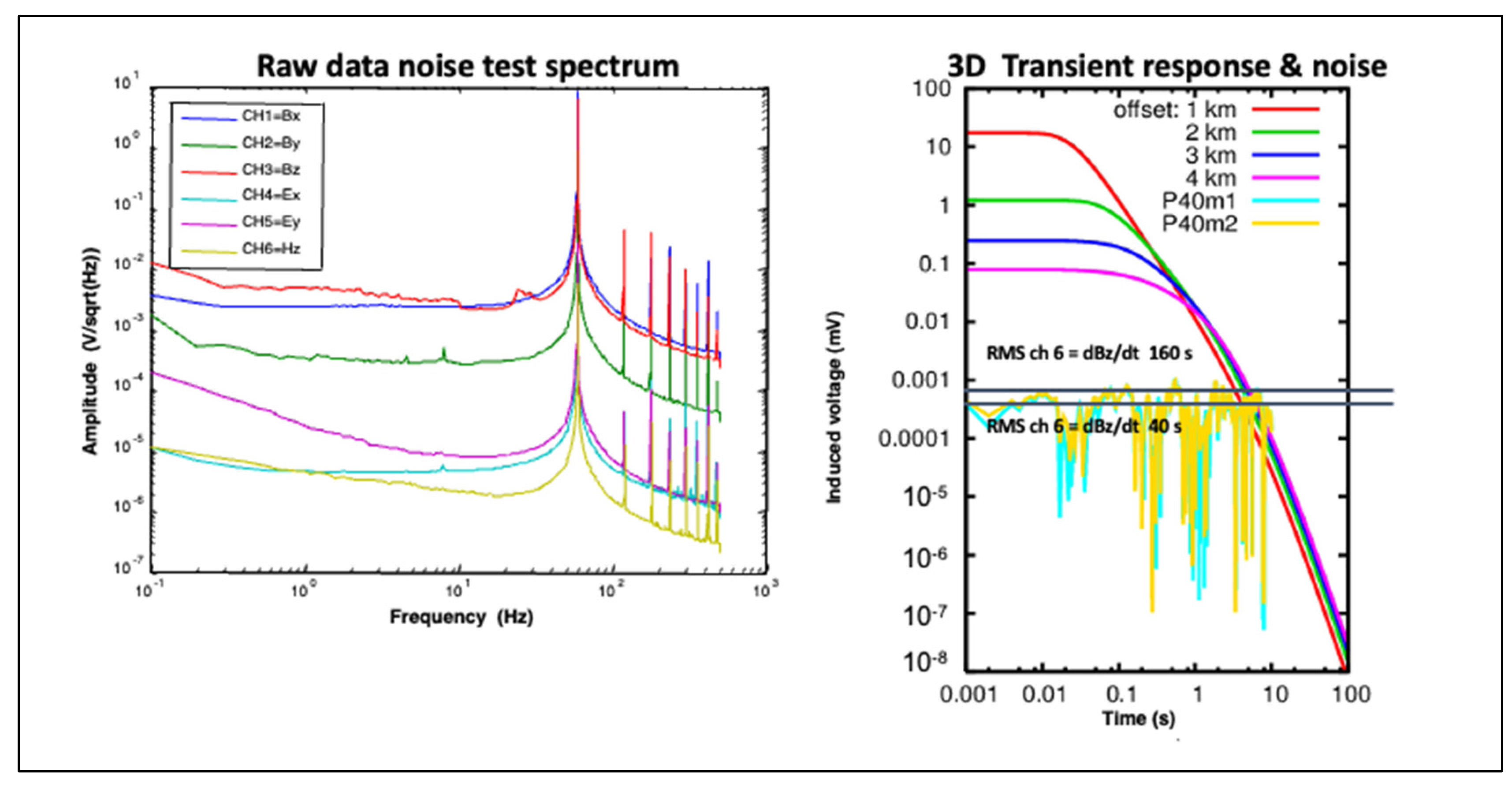
Concurrent with the 3D modeling, field measurements were conducted near the potential injection plant to assess noise conditions. This allows optimization of the survey design and estimation of the data’s signal-to-noise ratios. Magnetic field sensors, electric sensors, and recording units were used in the test. An example of the amplitude spectra of the noise measurements is shown in
Figure 14. The amplitude of the noise recorded by the induction coils was higher than the air coil’s noise. This difference suggests that the areal averaging of the air coil reduces some of the localized noise (we did not see the same at different survey sites). The 60 Hz noise and its harmonics observed in the raw data were attenuated as part of the data acquisition/processing. Subsequently, the receiver data were used to simulate noise combined with the transmission cycle and signal processing. A CSEM transmitter’s response was modeled for four transmitter-to-receiver offsets used in the field using the 31-layer anisotropic model. The analysis shown yields stacked data as an excellent noise-level estimator on the right of
Figure 14. The resulting estimated optimum recording for CSEM data acquisition is 3:40 h. This proved very useful during the 24-rotation acquisition (a minimum of 4 h of recording time was used depending on local noise conditions and real-time quality assurance).
For the MT acquisition, the skin depth formula and the estimated lowest frequency at approximately 3000 m deep were used to derive the recording time for the MT data acquisition. The high frequency (HF) range includes power line noise and uses HF data processing, and the low frequency (LF) range is below the power line noise and uses LF data processing (all robust processing). This range was used for overnight data acquisition. The duration variation depended on when the station setup was finished and when the station was moved the next day.
2.1.2. CSEM and MT Data Acquisition
Based on these feasibility study results, a time-lapse CSEM monitoring project was designed. The survey layout and design are shown in
Figure 12. The baseline survey was taken before the CO
2 injection into the formations. Furthermore, an MT survey was performed in conjunction with the baseline CSEM survey to measure field site background resistivity. The survey was carefully designed, and special attention was paid to noise levels in the field to ensure that any time-lapse differences observed would be solely due to changes in CO
2 concentration within the reservoir. All acquisition hardware was carefully controlled for variations and calibrations were conducted before, during, and after the survey. Long-term stability was shown to be better than 0.5% in the worst case (1 out of 14 instruments).
The initial EM surveying lines were designed to overlap the 2D seismic lines recorded in the study area. Protected areas were avoided when setting out the lines, and most stations were located at least 100 m away from power lines to avoid disturbance from EM noise. The survey layout consisted of three lines of receivers and two separate CSEM transmitter sources to the north and south, each with two dipoles. Given the optimal 200 m station spacing as determined from the feasibility study, 125 CSEM receiver locations were used. The receivers consisted of 100 m long dipoles oriented north–south (Ex) and east–west (Ey). An air loop or buried induction coil was laid out on the northwest quadrant of each receiver site to measure the vertical magnetic field (Hz). Contact resistance was logged at each site for quality assurance during acquisition, processing, and interpretation.
CSEM in the time domain was selected for this project because of its high sensitivity in onshore applications (e.g., [
15,
46,
47,
48]). CSEM with grounded electric dipole excitation is better suited for reservoir analysis since the grounded transmitter excites horizontal and vertical currents in the formation, making the method sensitive to thin anisotropic resistors. However, in CO
2 monitoring, sensitivity to both resistors and conductors is needed; namely, a full 3D anisotropic model [
23].
Each source consisted of buried electrodes connected by a 1 km cable to the transmitter. The transmitter was set to transmit between 160 and 250 amperes of current. The actual current was monitored and recorded during transmission to normalize the data. The recording times for each receiver station were between 4 and 5 h. Extended long recording times (total of 7 h per transmitter) were conducted at overlapping sites for use as reference locations should later time-lapse processing require this.
The total frequency range of MT data can be from 40 kHz to less than 0.0001 Hz, depending on the equipment used (here, we mainly used up to 1 kHz and sometimes up to 20 kHz). The ratio of the electric (Ex, Ey) and magnetic (Hx and Hy) recorded values gives an estimate of the apparent resistivity of the Earth at different depths. This estimate can be used to differentiate between rocks with contrasting resistivities, such as sandstones saturated with brine, and those where CO2 has been injected.
Forty-two MT site locations were deployed, as depicted by large green dots in
Figure 12, with a spacing of 600 m between each MT recording site. Three planned stations near the power plant were skipped during the survey because of noise/access issues. Six additional sites were located close to a noise source; the recorded data were reviewed in these cases, and the measurements were repeated because of unsatisfactory quality. A primary remote reference site was in Grand Forks, North Dakota, and a backup site was operated in Austin, Texas. MT data quality was greatly improved by using the remote reference during data processing.
Quality Assurance/Quality Control
Quality assurance/quality control (QA/QC) procedures were performed both in the field during collection and after data processing. Additional measures were considered when the receiver sites were in relatively high EM noise areas, including carefully selecting the appropriate electric line length when laying out the site, extending data acquisition time, and conducting necessary repetitions based on closely monitoring daily operations.
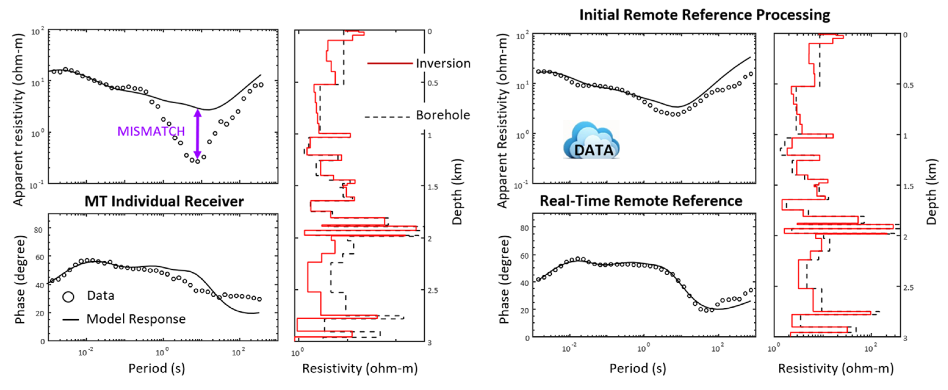
For MT measurements, the data were uploaded to the Cloud, and results were returned the following day, including remote reference processing where available. An example is given in
Figure 15. The single site processing on the left still shows a mismatch between data (circles) and the inversion model response (line). This difference was caused by local low-frequency noise, which was almost wholly removed when applying remote reference processing [
49].
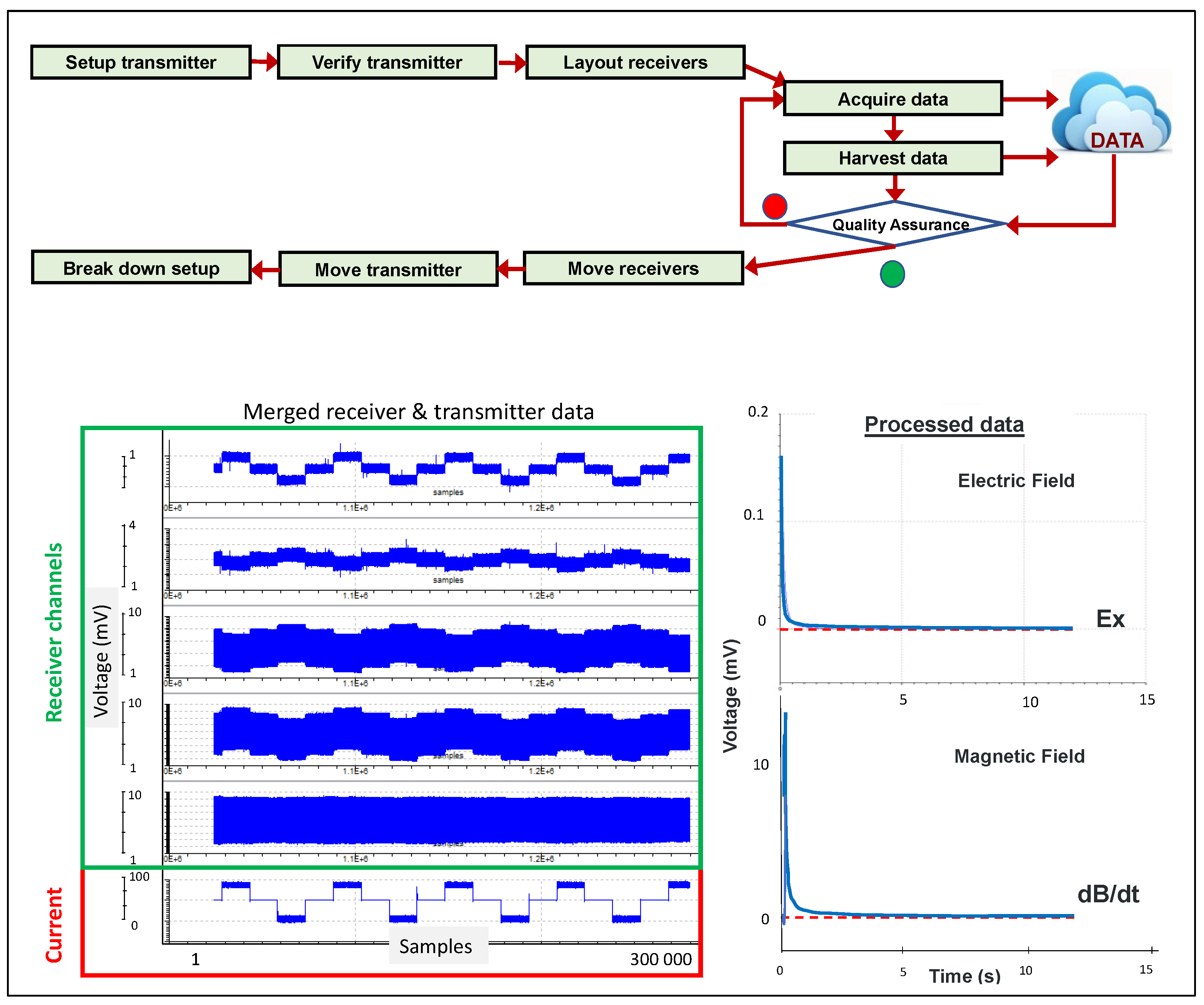
Figure 16 depicts the CSEM field workflow using cloud services for real-time data quality assessment. Data were uploaded to the Cloud for quality assessments during 24 h field operations. Since the inversion is based on electromagnetic fields, we only conducted quality assurance of the voltages. This also allowed us to QA the data without normalizing the transmitter current and operation parameters (time-consuming). If a receiver station showed poor data quality, the station was investigated, and the measurements were repeated until the quality improved. Examples of high-quality transmitter and receiver data are depicted in
Figure 16. This workflow was fundamental to maintaining high data quality while monitoring acquisition equipment moved along the survey line (leapfrogging). High source/receiver repeatability was obtained, with an error difference of approximately 0.5%.
CSEM and MT Data Processing
After passing initial QA during acquisition, transmitter and receiver data were merged into matching the transmitter–receiver pair files. This process also included time alignment between the transmitter signal and receiver data, a correction for time shifts, and the current waveform. Once all input parameters were verified (including onset time, transmitter current used for normalization, waveform period, and type of waveform), a three-point delay filter was applied to ensure waveform symmetry. Initially, we tested parameters with various other filters described in [
22,
48,
50,
51], but in the end, there were sufficient statistics that stacking rejected most noise.
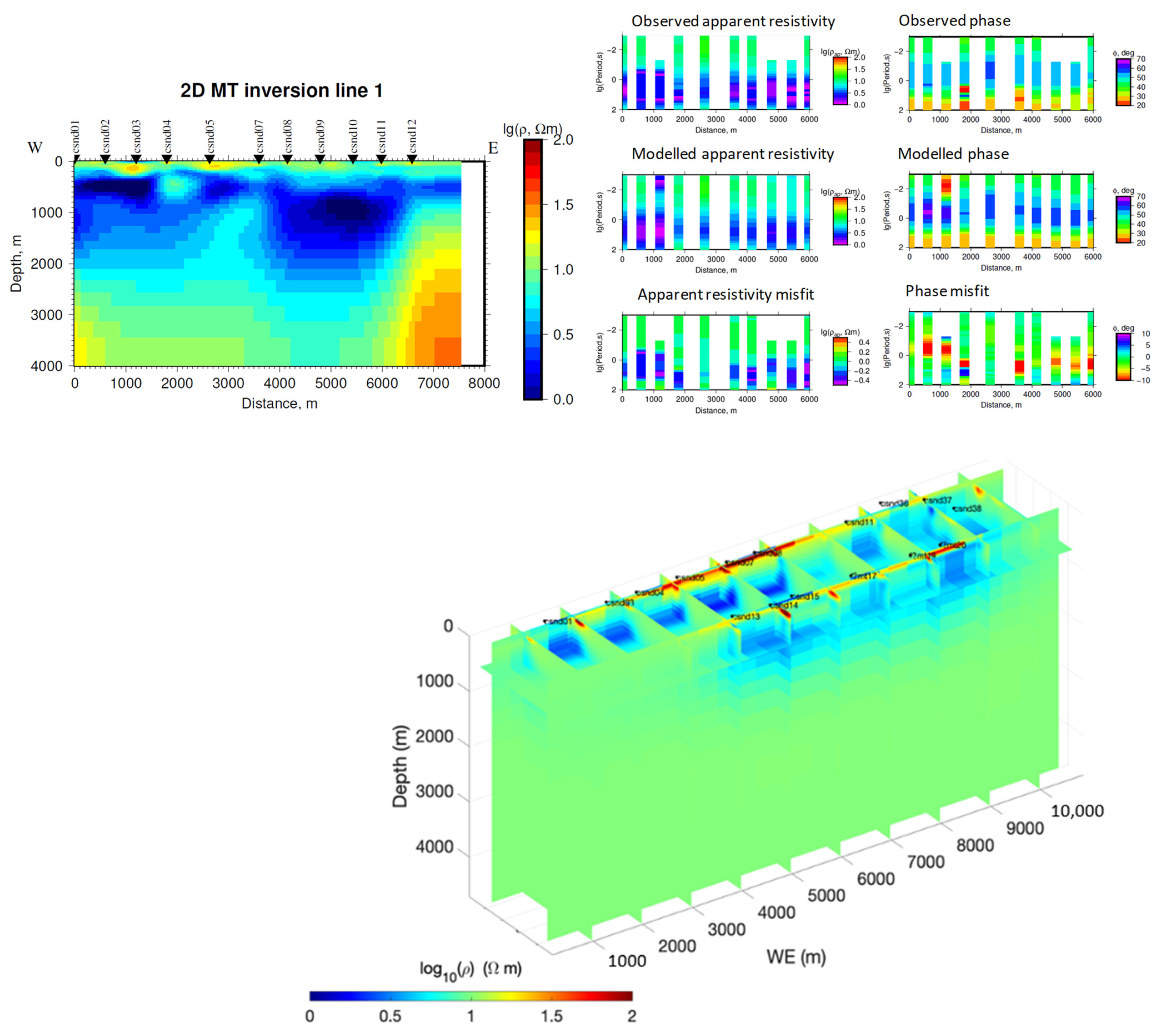
For the MT data, we obtained an apparent resistivity and phase curve for each location that was of acceptable quality. This was carried out more carefully at the post-acquisition time with a more detailed analysis. Two-dimensional inversion was applied to the data to generate a resistivity model along the profile, as shown in the top part of
Figure 17. These 2D models were the starting 3D resistivity model used for the 3D MT inversion, with an outstanding result shown at the top left and bottom of
Figure 17. Notice the lateral and vertical resistivity variations in the profiles. These results reflect the MT method’s sensitivity to the study’s geologic conditions and the data quality.
In postprocessing, the time-series data were evaluated for data quality. The data were categorized as excellent, good, noisy (acceptable), or poor, depending on the pattern and rate of both magnetic and electric transient decay. All categories of data may additionally show transient reversals (zero crossovers), suggesting the possible presence of signal channeling or 3D structures. Because of the careful field data collection process, approximately 85% of the collected data were classified as good or excellent. Another 6% could be further processed to reach that level of quality. For a field CSEM data set this large, this is a high level of data retention and nicely sets up future time-lapse surveys for success. An unconstrained 1D inversion was performed for each receiver site, and the error bars from the stacking were used as data weights in the inversion. After paying careful attention to the distribution of the eigenvalues of the inversion model parameters, we removed more data restrictions and a priori constraints as the eigenvalues were statistically distributed, meaning the data were sensitive to 3000 m depth. The results were compared to an anisotropic borehole resistivity model to validate the data further.
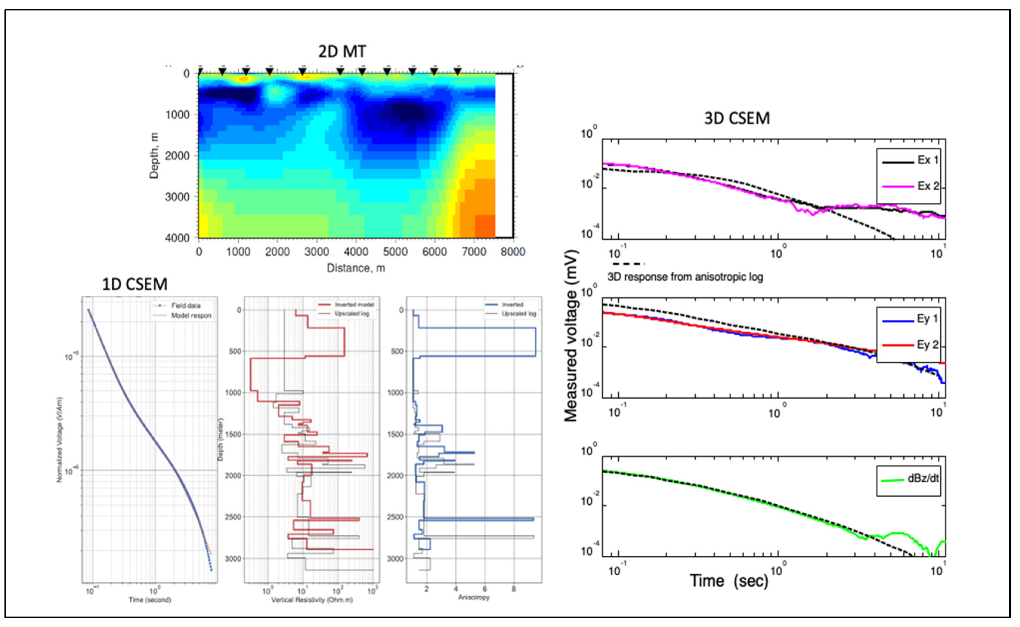
Figure 18 compares the one-dimensional CSEM inversion to the two-dimensional MT inversion for Line 1 (northern E-W profile) and the three-dimensional modeling results, including the seismic horizons. The CSEM data in this inversion are from a representative site on the 2D MT inversion section. The borehole log is represented in black, while the CSEM inversion models and the anisotropy coefficient are in red and blue, respectively. It is worth noting that the inversion was performed unsupervised with a half space of 31 layers as the starting model. The inversion results match the log well. The panel on the right shows the comparison of the data with the 3D model response, including the log and adjusting the model depth by the seismic horizon depth at that site. The 3D model response on the figure on the right (dashed line) fits the data well in all components except for a later time in the Ex component when the signal disappears in noise, as this component is weaker due to transmitter symmetry consideration.
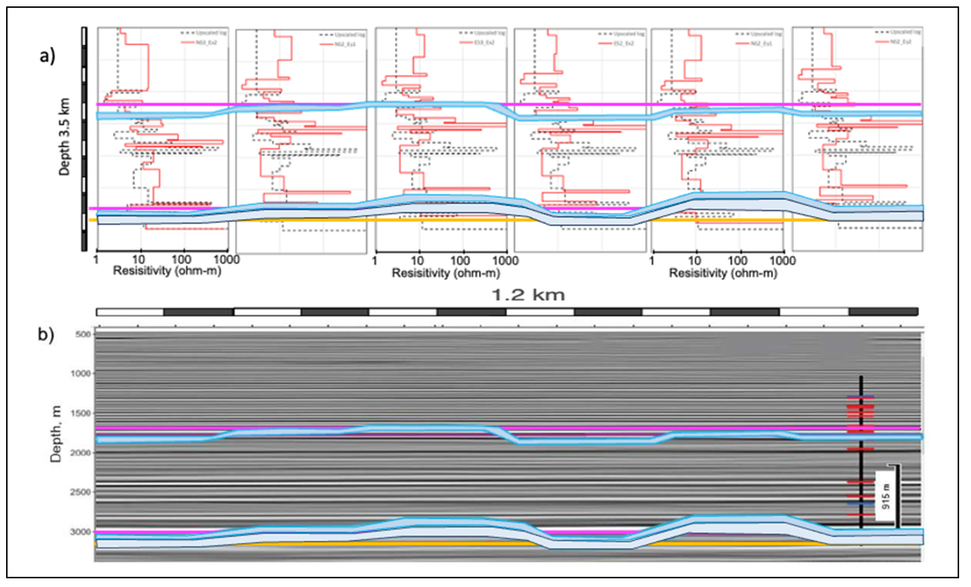
1D inversion results (in red) and the borehole model (in black) of eight sites adjacent to each other along Survey Line 2 and Transmitter 2 (south) are shown in
Figure 19. Generally, inversion results align well with the borehole data, indicating high confidence levels in data collection and processing. The shaded outlines indicate the interpreted Broom Creek and Deadwood formations from the inversion results. Further results were validated by comparing the inverted resistivity models with 3D seismic data with the Broom.
Creek and Deadwood seismic horizons (in the bottom part of the figure). For most stations, the CSEM inversion accurately matches the seismic model. Inversion results that deviate from the seismic model could indicate lower data quality or denote areas of 3D structure unaccounted for in 1D inversion. Based on independent, unsupervised 1D inversions (starting model is a half-space), these results confirm the quality of the CSEM baseline measurements.
2.2. Geothermal
In 2021, global use of geothermal energy for thermal applications increased to approximately 141 terawatt hours (TWh), while direct use of geothermal heat reached about 128 TWh. However, the global distribution of geothermal energy use for power generation and heating/cooling remains sparse, with at least 82 percent concentrated in a few countries such as China, Turkey, Iceland, the USA, Japan, El Salvador, New Zealand, Kenya, and the Philippines [
52,
53]. With its vision for 2030, Saudi Arabia recognized and began diversifying its economy and reducing its reliance on fossil fuels. Therefore, developing renewable energy sources, including geothermal resources by 2030 and net zero carbon emissions by 2060 [
54], is a top priority.
Geothermal resources in Saudi Arabia are promising. Several exploration campaigns and research studies have investigated Saudi Arabia’s geothermal resources for decades [
55,
56,
57,
58,
59,
60,
61], with a couple focusing on the Al-Lith area in southwestern Saudi Arabia [
62,
63,
64,
65]. The Al-Lith area has four hot springs with surface temperatures ranging from 41 °C to 96 °C, with Ain Al-Harrah having the highest. The Ain Al-Harrah hot spring’s geothermal reservoir is characterized by a high surface temperature of up to 96 °C and favorable petro-thermal characteristics of 185 °C (reservoir temperature), 219 kJ/kg (discharge enthalpy), and 183 mW/M
2 (heat flow) to provide long-term electricity to the Al-Lith area. Due to limited geophysical measurements in this area, these claims require further verification. We report here only the initial findings of the MT measurements, which are used to plan a more detailed CSEM survey later to drive future new drilling targets. Notice the primary targets for geothermal energy are conductive, while for CO
2 monitoring, the CO
2 plume is resistive. Therefore, MT plays a more critical role in geothermal energy than in CCUS. However, both cases require all EM components from the MT and CSEM methods to differentiate the fluid signature from the surrounding host rock.
Thirteen MT stations were collected using non-polarizable electrodes, and low-frequency induction coils. This data acquisition system used in a 40 °C environment in Saudi Arabia is identical to the equipment used in the North Dakota CCUS example mentioned above at −20 °C. The data were acquired for about 7 h at three different sampling frequencies of 4 kHz, 1 kHz, and 40 Hz. The raw data were processed in detail to ensure high-quality results. This stage involved a spectrum analysis and coherence to examine the relationship between two orthogonal and parallel fields. The impedance tensor was estimated using a robust statistical technique. The multiple impedance tensor results were further processed to extract the final transfer function data. Finally, the impedance tensors were inverted using a smoothness constraint algorithm for better image and interpretation.
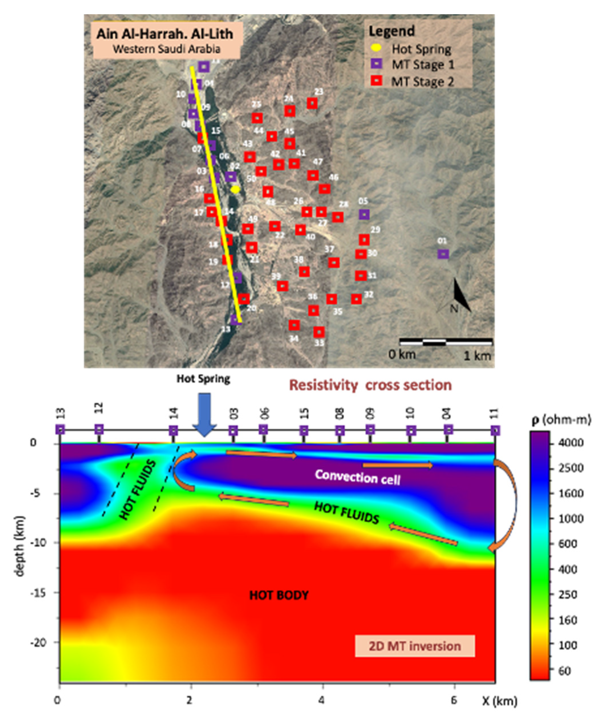
The final 2D inverted section along the N-S profile (blue sites) in the study area is shown in
Figure 20. The selected subset shows the flow and the reservoir best. The remaining data acquisition is ongoing and will be subject to a later complete analysis. The preliminary results of this MT study are the following:
The geophysical survey detects and clearly maps the heat source, a low-resistivity hot body below a depth of 7 km.
The geothermal flow cell observed at the bottom of the figure (hot fluids—green area) consists of the fractured basement acting as the pathway for the geothermal fluids to reach the surface.
The heat exchanger is represented by the whole system, where the heat transfer consists of conduction through the hot body and convection via the flow cell.
A fluid cell of lower resistivity and a deeper heat source can be identified from the MT data. The blue arrow in the figure indicates the location of a known hot spring as a reference.
Future activities in this project include other geophysical measurements (gravity, passive seismic, CSEM) with denser station spacings and data integration.
2.3. Enhanced Oil Recovery (EOR)
Imaging a flood front can often increase the EOR recovery factor by 30%–50% [
23], which means less carbon footprint per barrel produced. When using CO
2 as a driving gas, one can obtain further carbon credits and move toward CO
2-neutral operations. From an EM plume imaging sensitivity viewpoint, EOR lies between CCUS and geothermal energy, as in most cases an unbiased resistivity of the fluids at the boundary of the flood front is needed. The first example is a heavy oil application where oil reservoirs are often shallow and expensive, and steam is used to drive the oil. This scenario represents a resistivity contrast at the flood front that would be replaced in case of CO
2 flooding with a short conductive front followed by a resistive CO
2 plume. The second key issue in the EOR case is the ability to record EM signals through the casing. This issue can be overcome by using a surface-to-borehole configuration. Another typical EOR case is waterflood, where a strong contrast between the resistive oil and the conductive water is present. We show a field example for this supported by 3D modeling.
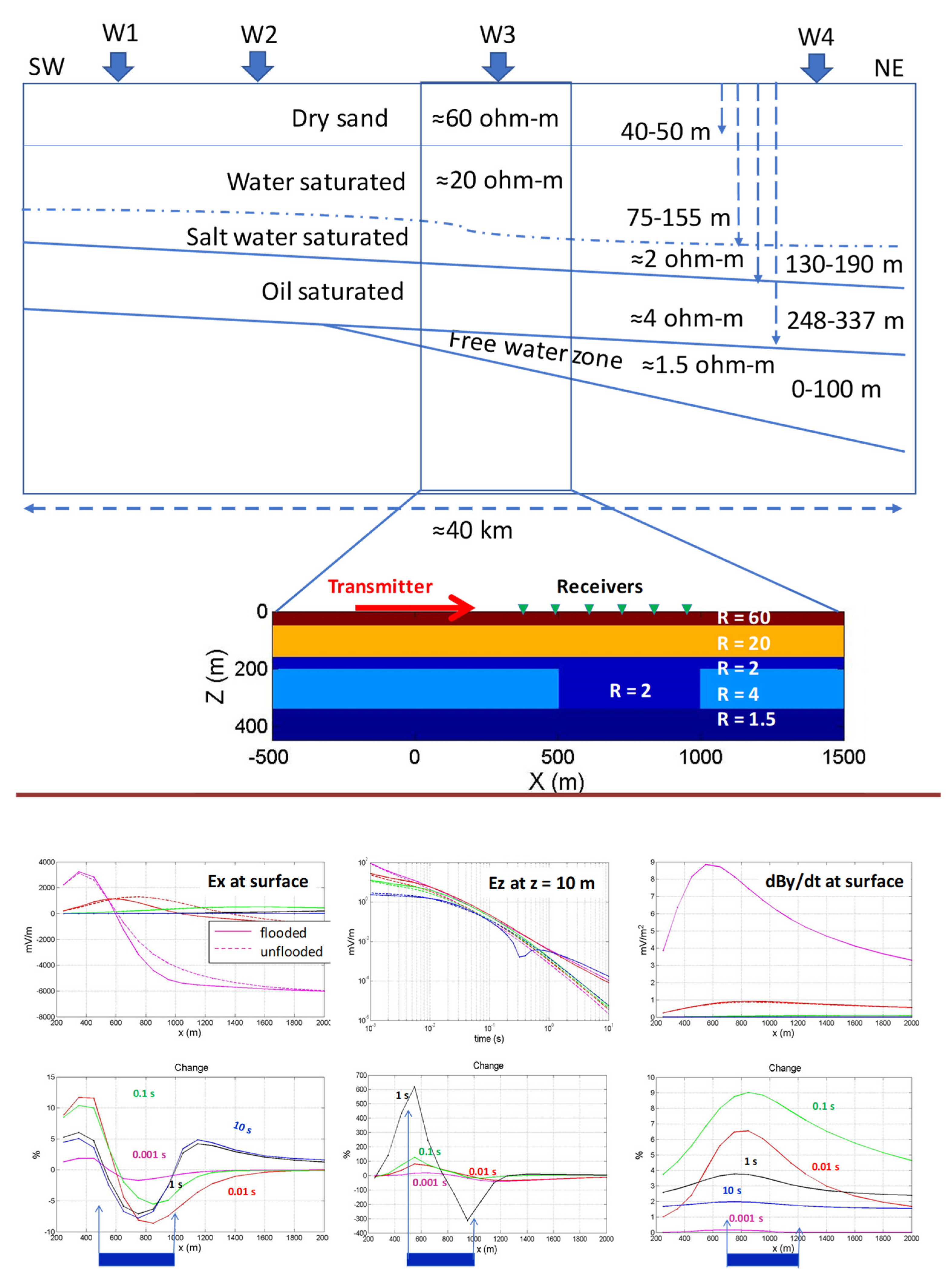
Figure 21 shows a typical resistivity section for a heavy-oil (HO) reservoir in the Middle East. In this case, the oil reservoir is shallow, around 250–350 m depth. The oil is routinely driven by expensive steam (conductive oil–water contact—OWC). Using CO
2 would add carbon credit to the equation and produce resistive oil–gas contact (OGC). The critical considerations are to map the HO reservoir versus the free water zone below, which is a conductive target, and to map oil leaks from the HO reservoir into the upper aquifer, which is a resistive target. Thus, all EM components are required. We modeled these scenarios using shallow borehole measurements as they provided a better image of the anomaly [
66]. The results are shown at the bottom of
Figure 21 with the electric field in line with the transmitter, Ex, the vertical electric field, Ez, just 10 m below the surface, and the time derivative of the magnetic field dBz/dt at the surface. The top curve represents the field values flooded and unflooded (dashed) and below the percentage variation for different times after turn-off. The water flood is clearly seen in all curves—slightly smoother for the magnetic field and most expressed for the vertical electric field. This is because of the focusing effect that shallow boreholes show.
After obtaining large anomalies with shallow boreholes, the next step in the modeling exercise is to assess the EM response when the boreholes are connected to the surface. This is because much larger source moments and signals at the surface can be more easily generated than in the borehole. Furthermore, a better signal-moving receiver in the borehole can be obtained as they are more protected from surface EM noise.
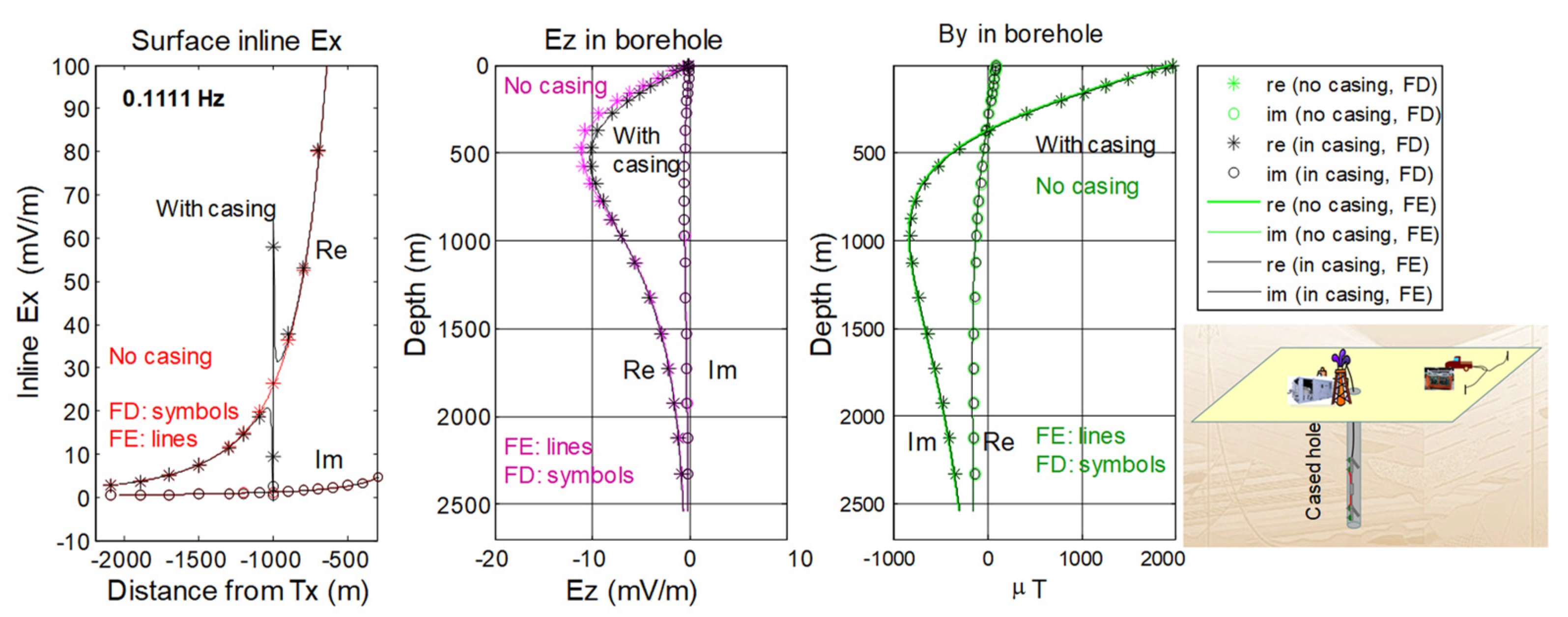
Figure 22 depicts the surface-to-borehole concept with a transmitter at the surface (sketch on the bottom right of the figure). In this figure, the same components as in
Figure 21 are analyzed, except this time in the frequency domain (casing effects are frequency-dependent), where real and imaginary parts of the solution can be compared, with and without steel casing, and using Finite Difference (FE) and Finite Element (FD) software codes. Here, we compared FD and FE codes. Their responses were in good agreement. The electric and magnetic fields in the borehole give additional insight into the required measurements. To a depth of 2500 m, the signal level from a surface transmitter is well above the noise floor. For magnetic field components, sensors already in production can be used. The magnetic field is in the micro-Tesla range, while typical fluxgate sensors have a 3–6 pico-Tesla noise floor. Therefore, extending the borehole sensors from a shallow borehole tool to a deep one is feasible.
This example shows that it is possible to obtain meaningful data from the surface, and borehole sensors can contribute with a good EM response using existing technology.
The second example illustrates the surface applications using test measurements from an oil field.
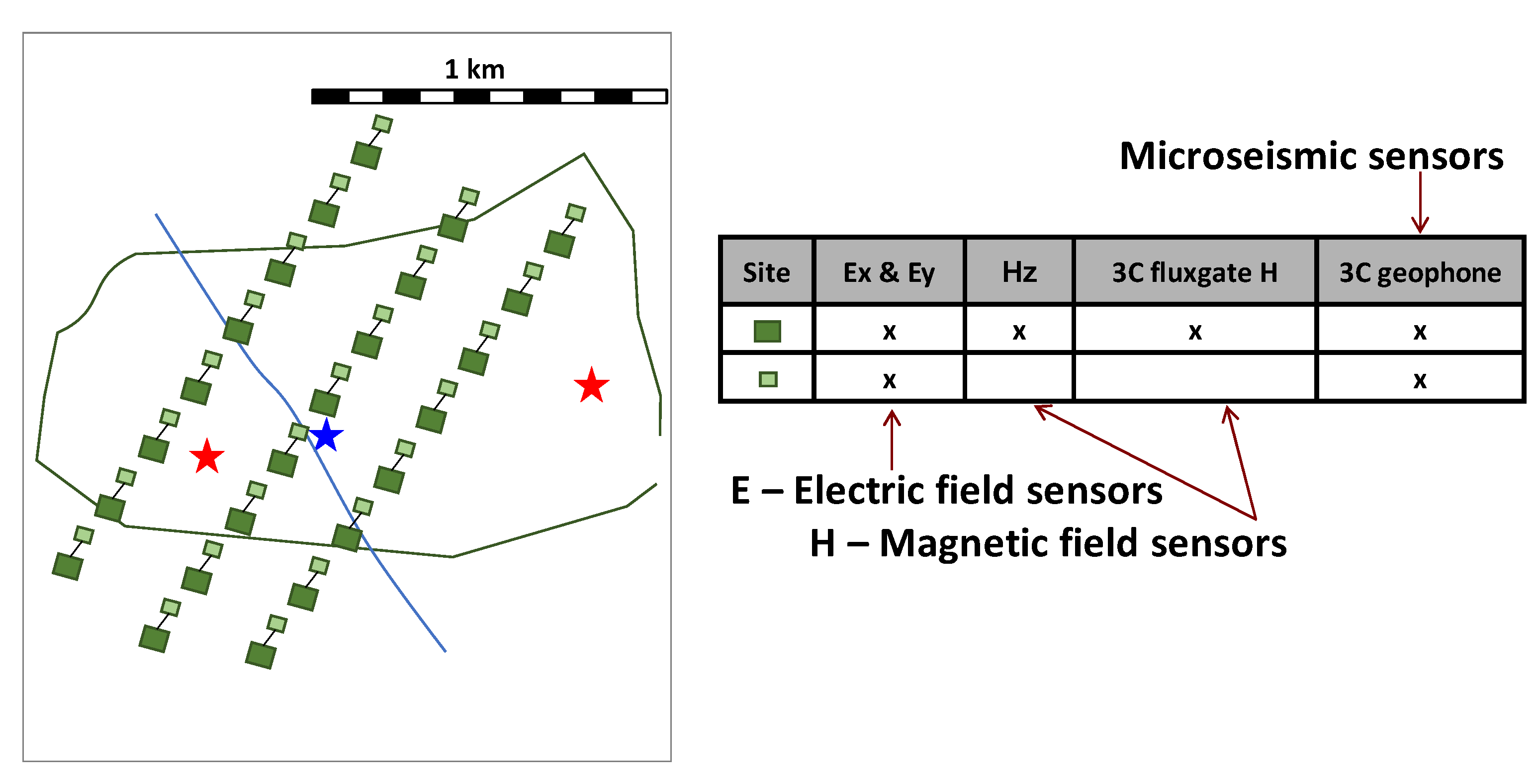
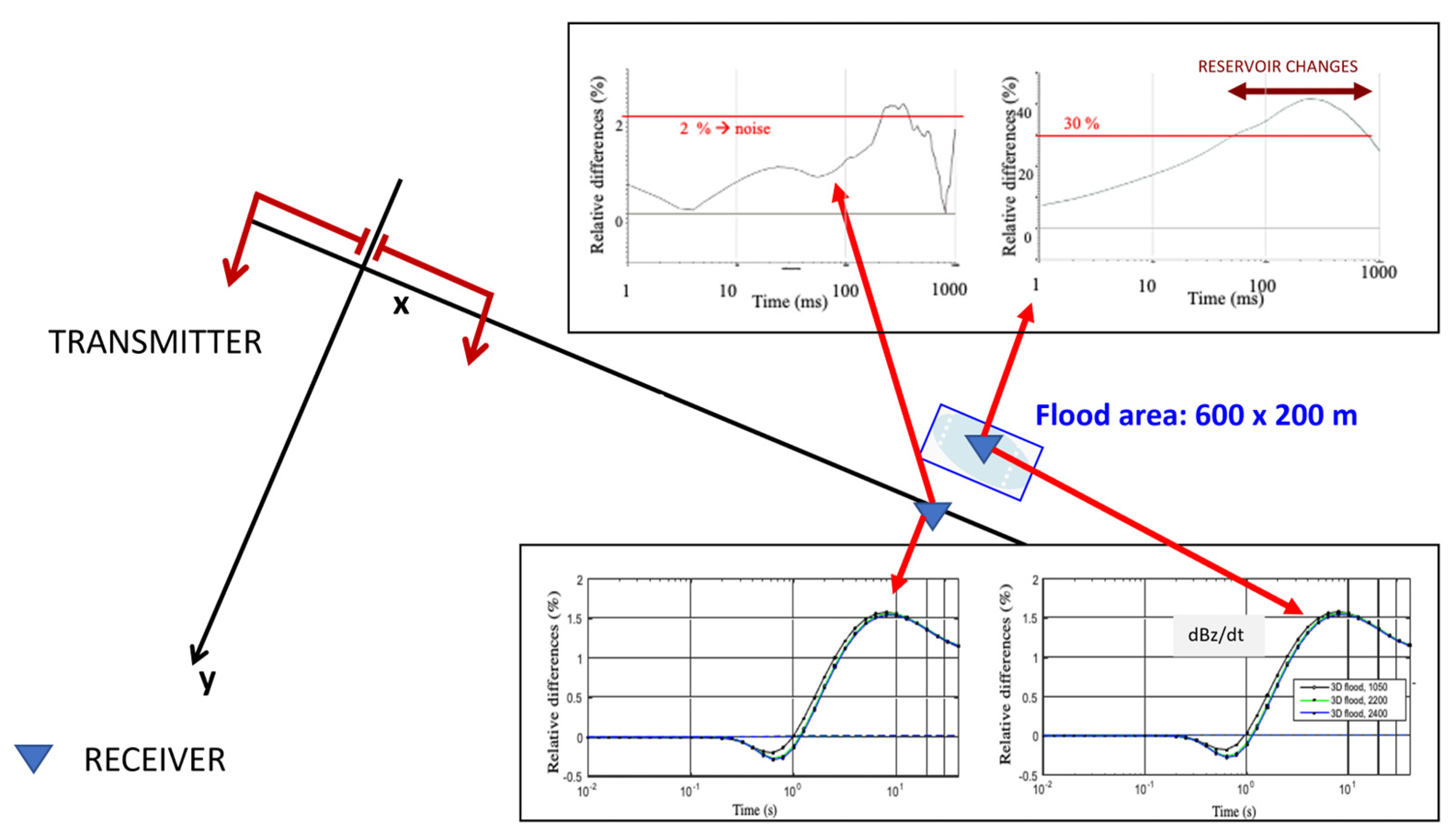
Figure 23 shows an exemplary layout across a reservoir (gray outline) with the flood front surface projection shown by the blue line. Ideally, one would deploy as many receivers as possible, but cost/logistics limitations often only allow limited use. Microseismic receivers were included as microseismic data can be easily acquired with the same data acquisition system.
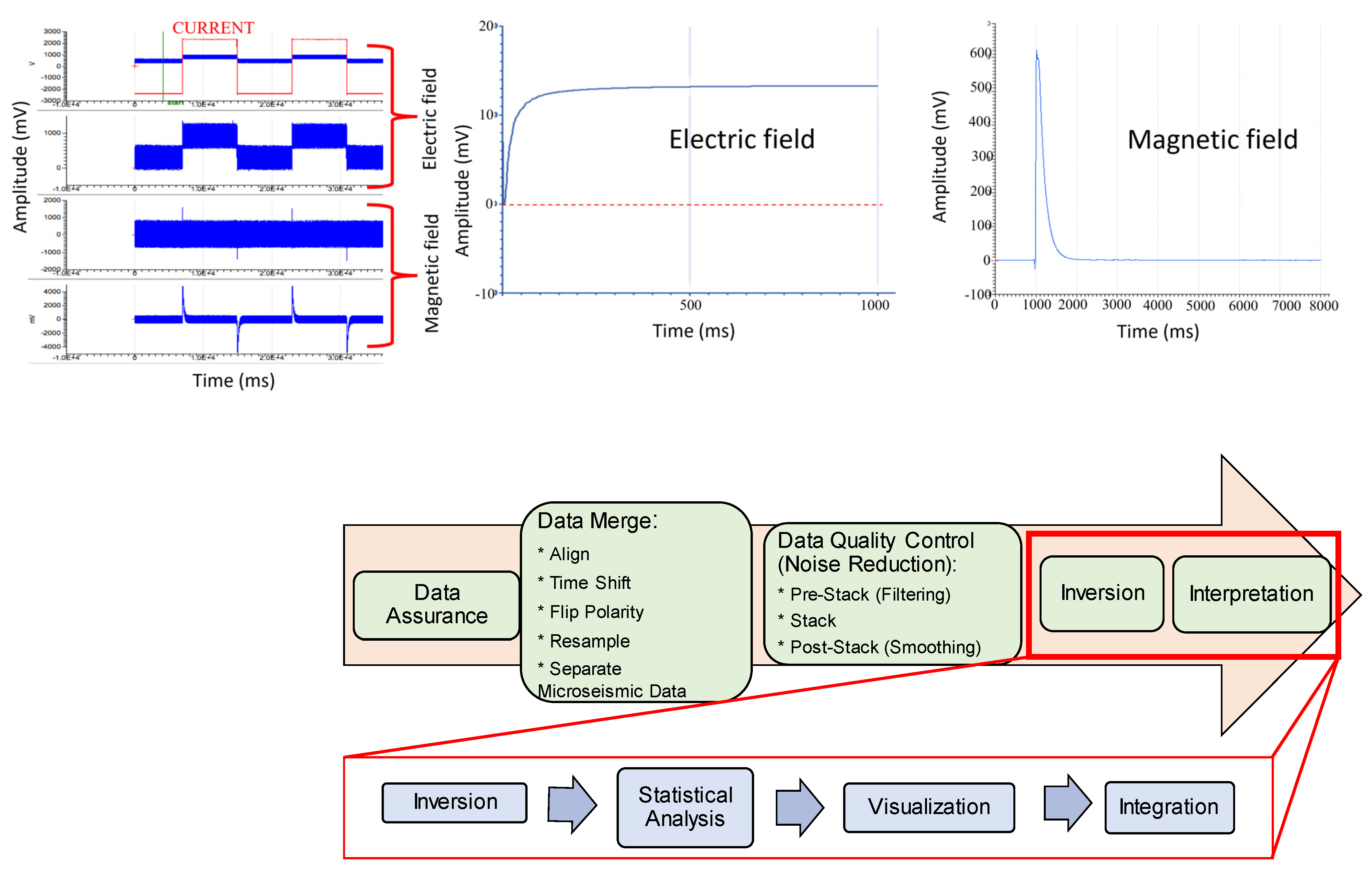
Figure 24 shows some test data from a water flood field test. The raw data are aligned with the transmitter current, and the seismic traces are moved to the seismic processing. The electric field at the top left of
Figure 24 follows the transmitter current. The magnetic field shows the transients resulting from the transmitter and the noise recorded by the receivers. The top right depicts the stacked signal before and after filtering. In the figure’s middle and bottom row, the flowcharts for processing and inversion/interpretation, respectively, are shown. In this survey, the generator noise had to be filtered out during the data processing. The field tests started with careful site selection and feasibility analysis, as described in the CCUS example.
The results from the field trial are shown in
Figure 25. The survey layout was a 1 km long transmitter and several receivers crossing the waterflood at a 2.5 km distance. One receiver is directly above the waterflood, which consists of water injection at 2 km depth from horizontal wells. The second receiver is 400 m away from the first one. Displayed are the time derivatives of the magnetic field as a time-lapse difference in percent over approximately 50 h. Whereas the receiver directly above the water flood showed a 30% anomaly, the second only showed 2%, which we attributed to noise (our threshold in this experiment). The same responses from 3D modeling of the survey results at the bottom of the figure only showed about a 3 to 5% anomaly. Three-dimensional models, including the horizontal well casing and infrastructure, could not explain the difference via modeling. One of the two possible explanations is current channeling, where the induced transmitter current is channeled into the water flood as it covers a sizeable subsurface volume. Another possibility is the flood front related to the pore fluid mechanism described in
Figure 1. When the flood front replaces fluid, it exerts forces on the old pore fluid, which causes localized alignment of the saturation water and, subsequently, an abrupt resistivity reduction. Further data on this are outstanding.
2.4. Critical Minerals—Lithium Exploration
As discussed above, lithium applications require the same EM technology as in the other case history examples. Mature lithium deposits can be found in Latin America, China, Australia, and the USA, and emerging deposits can be found in Europe and the Middle East [
17].
2.4.1. Lithium Exploration in Argentina
In total, 65% of world reserves are in the so-called lithium triangle located in Argentina–Bolivia–Chile. This area hosts salt flats with brines that contain this mineral [
69].
Due to the growth of the lithium market, the exploration frontier is changing, and currently, it extends to new concepts that drive toward the exploration of clay deposits with anomalous lithium concentrations, with much shorter production times from brine resources; fractured basements saturated with brine; and deep targets [
69,
70].
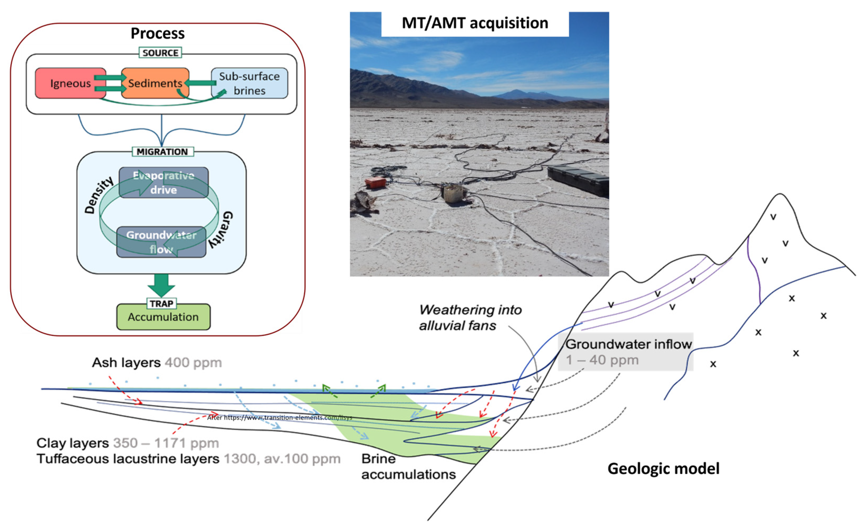
Figure 26 shows a summary of the process leading to lithium deposits. The minerals from mountain ranges combine with water and reach salty flats, where they build salt flats. A field setup of the equipment is shown at the top.
The elements of the lithium-bearing systems require deep imaging of the endorheic (i.e., closed) basins. Geophysical variations, such as low electrical resistivity in salt concentrations, low acoustic impedances, and dynamics of the hydrogeological system, make brine exploration a complex problem. Operationally, the situation is not better because the Argentine salt flats are in sterile areas, at altitudes of 3600–4200 m and more, and, in many cases, in hostile environments with difficult accessibility and surveying. EM methods are better suited for high-conductivity targets, such as lithium brine with low resistivity (typically 0.1 to 0.5 ohm-m), than DC resistivity methods. Due to its limited dynamic range, this resistivity contrast at depth is also challenging for conventional mining and groundwater prospecting equipment.
Curcio et al. [
70,
71] analyzed different geophysical responses (seismic, magnetics, electric, EM, and gravity) in salt brine exploration. Various feasibility studies, field tests, and previous acquisitions were analyzed, and new acquisitions in many salt flats were made. Full-tensor MT, gravity, and electrical resistivity tomography (ERT) are currently the best combination of geophysical methods to reach the exploration objectives: characterization of the salt flat in-depth, basement delineation, definition of the main structures and main faults with the section, and detection of semi-freshwater aquifers in the edge of the salt flat providing the recharge that is key to the water balance of the endorheic basin.
MT’s success in brine exploration relies on the low frequencies at which the MT method operates, compensating for the effect of the low electrical resistivity values in the skin depth relation. Sensitive to conductance, MT prospects the entire conductive column and characterizes the basement. Although the signal may be low, the equipment used in the case history here has patented amplifier behavior [
18] and outstanding storage capacity that provides sufficient data statistics, resulting in an enhanced signal-to-noise ratio during advanced data processing [
49]. On the other hand, a full-tensor MT provides extra interpretation attributes that cannot be achieved with other EM methods [
70,
71].
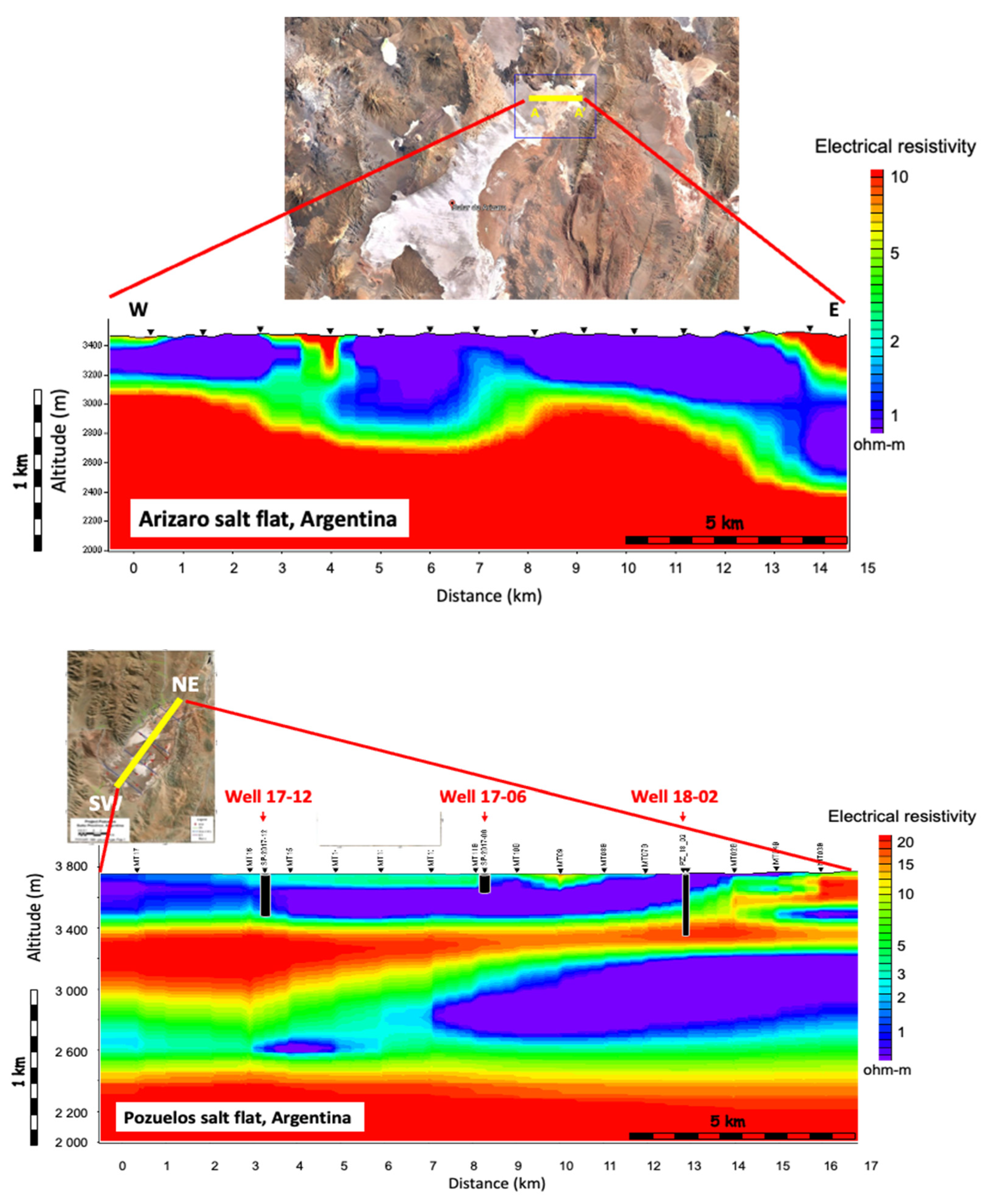
Figure 27 shows the MT response in salt flats. The complete study corresponds to a multi-measurement (full-tensor MT, Gravity, and ERT) survey where the geophysical model was obtained by integrating geophysical data with well data to build a 3D static model and a 3D dynamic model used in the resources and reserves estimation.
The MT frequency bandwidth is from 0.001 to 50 Hz. In both interpretations, the polar diagrams and skew indicate a 2D/3D dimensionality, and the MT section is divided into three geophysical units: the highest electrical resistivity (in red) is interpreted as the basement; the electrical resistivity in blue-violet (with the lowest resistivity of 0.1 ohm-m to 1 ohm-m) is interpreted as brine-saturated rock or wet clay (only possible—in principle); and green (mid resistivity) interpreted as rock saturated with fresh water with a lower content of salinity than the violet unit.
The first example is in the Arizaro salt flat. During 2019, approximately 65 km of full-tensor MT data with a depth of investigation of 2 km were acquired.
Figure 27 (top) shows the 2D section of one of the ten lines. The MT section shows that the signal successfully passed the conductive unit that in the west has 200 m thickness, whereas the center-east model reaches 400 m depth. The model shown also delineates the shallower basement in the east (3000 m depth) and deeper in the west (2400 m depth) and main faults.
In the second example, approximately 50 km of full-tensor MT data with a depth of investigation of 2 km were acquired in the Pozuelos salt flat (bottom in
Figure 27) in 2019.
Figure 27 (bottom) shows the 2D section of one out of seven lines. Two conductive units, the shallower one from the surface, can reach 400 m thickness except in the NE of the area, where a fault indicates the end of the unit. According to the production wells, this unit couples a clastic or evaporite multilayer system where most of them are saturated with brine. The shallower portion of the mid-zone of the model has mid-resistivity values that indicate a zone of recharging with low-salinity water. The deeper conductive unit can reach a thickness of 500 m in the middle–NE part of the model. This unit and an important reverse fault are also detected in the crosslines. Still, we cannot affirm if its low conductivity is due to a deeper multilayer system saturated with brine or if it is due to wet clay (unlikely) because the wells are shallower than 500 m.
2.4.2. Lithium Exploration in Saudi Arabia
Active and passive electromagnetic surveys (CSEM-LOTEM and MT) were conducted in the Half-Moon region of East Province in Saudi Arabia in January 2022 [
17]. A high-power CSEM transmitter using a 1 km dipole was installed for the energy transmission, and seven receivers for both active and passive EM measurements were deployed at various distances from the transmitter, ranging from 930 m to 20 km. A 250 kVA generator was connected to the transmitter’s switch box to inject current through the electrodes. The injected current varied between 40 and 200 Amperes. In addition, the duration of the injection current varied between 5 and 30 min. Four electric field electrodes (Ex1, Ex2, Ey1, Ey2) and three magnetic coils (Hx, Hy, Hz) were utilized for MT.
For the CSEM survey, two different acquisition geometries and protocols were used. The LOTEM standard CSEM layout with air loop, S20 coil, which measures the vertical time derivative of the magnetic field, and for the focused-source EM (FSEM), four electric fields with air loop. The objective of the FSEM method is to obtain deep vertical resistivity data with horizontal electric differential field measurements. FSEM enhances the conventional CSEM technique, which has significantly higher spatial resolution and provides resistivity data with greater depth [
66,
72]. The CSEM (active) measurements were recorded with a 1 kHz sampling frequency during the day and switched to MT (passive) measurements with a 40 Hz sampling rate at night. However, we also utilized MT data sampled at 1 kHz before and after the transmitter was turned on. Both measuring modes (MT and CSEM) displayed a clear signal for all E-field and H-field components installed.
During data acquisition, the recorded signal is the combination of the induced field for the passive source and injected transmitter current for CSEM with the effect of the signal generation process and the Earth’s response [
22,
73,
74,
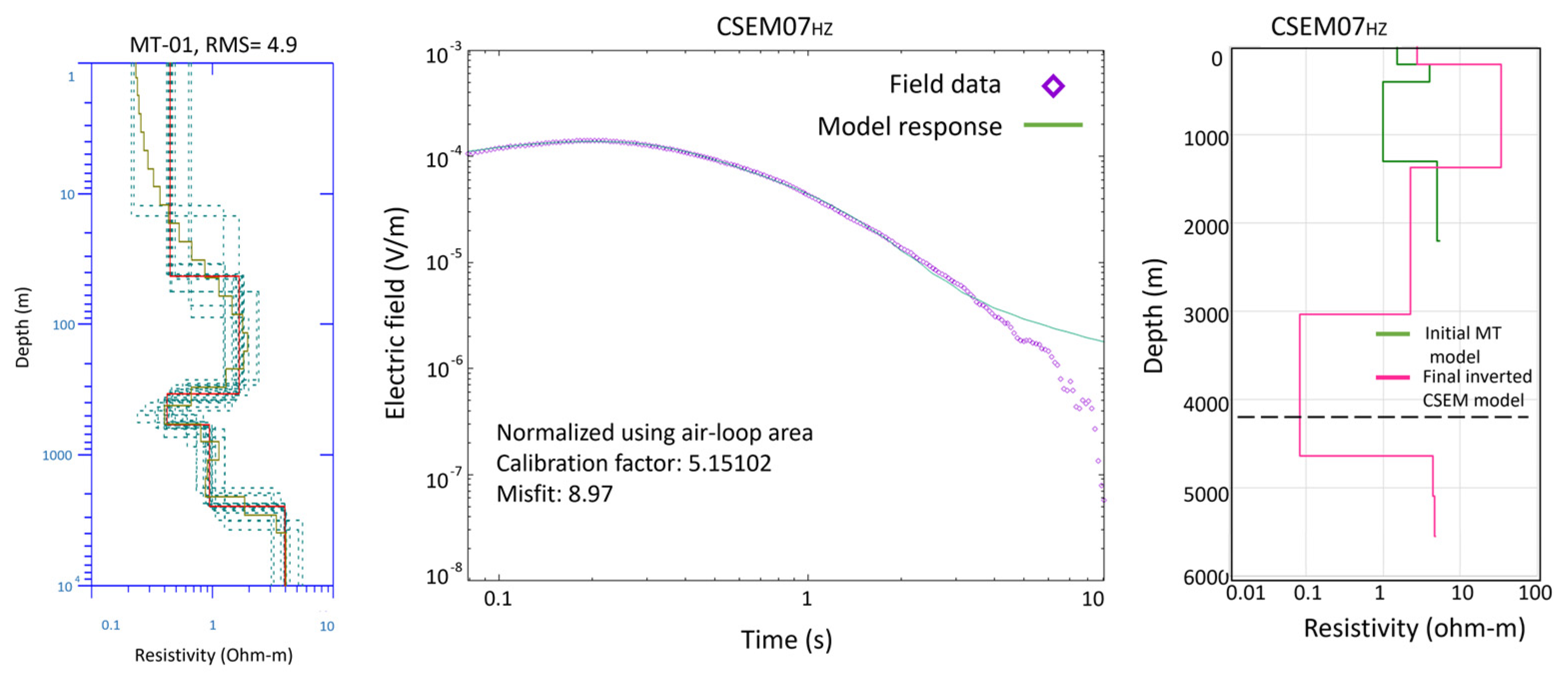
75]. Since two distinct EM measurements were collected, CSEM as an active method and MT as a passive method, the data must be separated and independently processed before they can be interpreted to create a unique subsurface model. The data were processed to perform data quality assurance and data quality control, including filtering. Since the records of the receivers contain both EM measurements with different frequency rates, these must be separated by cropping and merging before quality control processing. MT data generated the impedance, tipper, and spectral density matrices in EDI files conforming to the SEG standard. A one-dimensional (1D) analysis was performed on MT and CSEM (LOTEM) data for each sounding. The 1D inversion for MT data was performed for XY, YX, and the invariant of both data using Occam’s inversion technique. The 1D inversion results for MT data with RMS values between 1.3 and 5.3 for a 3-to-5-layer model were estimated. The 1D inversion for the LOTEM-CSEM data was also performed. Both electric and magnetic field data were inverted. Ultimately, both LOTEM and MT data inversion results were compared. The final inverted models indicate that the predicted model from LOTEM and the MT results agreed, as shown in
Figure 28. The fit of the CSEM data to the inversion models was generally satisfactory, falling within 1.5% root-mean-square deviation (RMS).
All MT data closest to the transmitter (Tx) were inverted using a five-layer model as a starting model, and the final inverted model exhibited similar behavior. In all four soundings below 300–350 m, a layer with a resistivity of less than one ohm-m was detected. The bedrock, identified as the more resistive formation, is two kilometers below the surface. The final inverted resistivity from the MT data at the same station was used as the initial model for the CSEM inversion. At a depth of 300–350 m below the surface of the Earth, a resistivity of approximately 0.3 ohm-m was observed, and a thickness of nearly 1 km was detected.
Similarly, the processed MT data collected 20 km from the transmitter (Tx) were used as the initial model for the final 1D inversion of the collected CSEM data in ST-07. Final inverted models for ST-07 are nearly identical, indicating that the data quality, 20 km away from Tx, was surprisingly high. At a depth of 1.65 km beneath the Earth’s surface, a layer with a resistivity of approximately 0.6 ohm-m and a thickness of nearly 1.9 km was detected.
The study area’s high-resolution MT/CSEM survey detected a very low resistivity anomaly with values around 0.3 ohm-m, similar to seawater resistivity. As no water layer is at depth, resistivities as low as 0.3 ohm-m can be linked to lithium deposits.
Both lithium applications showed unusually low resistivity. Future drilling will confirm the measurements.
3. Discussion
The concept of using CSEM for fluid imaging is based on a carefully designed workflow supported by a sensitive acquisition system. A critical aspect of the workflow is the flexibility to select numerous calibration points. The models and data are checked against a 3D anisotropic model derived from the logs at these points. This model—verified by 3D modeling—represents the ground truth. The feasibility analysis includes on-site noise measurements to determine the optimum survey parameters and acquisition time to obtain the best signal-to-noise ratios in the data.
We selected four energy transition applications (CO2 monitoring, geothermal, EOR, and lithium exploration) where this concept and the system architecture led to successfully reaching the objectives. At the CO2 monitoring site in North Dakota, we thoroughly applied the workflow and, under the inclusion of all logs, derived full 3D anisotropic modeling consistent with lithology, seismic data, and all other logs. The model serves as the ground truth for verifying data acquisition, quality assurance (near-real data quality check and acquisition operations control), and inversion.
For the geothermal example in Saudi Arabia, we used integrated geology and multi-measurement (EM [MT & CSEM], gravity, and passive seismic) information to overcome the lack of deep boreholes. The initial results already explain the known geothermal system around a hot spring area, and further data and interpretation are to follow.
Applying this workflow to EOR, where numerous boreholes exist in an oil field environment, brings challenges associated with the oil field noise and operation restrictions. The feasibility allowed us to design the field test so that we could overcome these difficulties and see the injection flood front after only a few days of recording.
The same EM system was applied to lithium exploration in Argentina (MT) and Saudi Arabia (MT and CSEM). In Argentina, the system could map existing lithium deposits. In Saudi Arabia, the MT and CSEM recorded at several locations showed unusually low resistivity conductors, strongly indicating that lithium deposits are possible.
In this CCUS application, both electric and magnetic fields gave comparable information. The magnetic field was more susceptible to noise. The information content down to a depth of 3 km was verified by analyzing the eigenvalues in the inversion. Due to the extensive calibration effect of the measurements, hardware, and methodology, the data were interpreted fully automatically, with the results matching the 3D model adjusted for the seismic horizons matching all CSEM components.
The EM application to EOR is more complex than for CCUS. In most cases, both electric and magnetic components are required. Also, the signal bandwidth is larger as the depth of hydrocarbon reservoirs can vary from a few hundred to a few kilometers. Resolution can be increased by adding borehole measurements. This is important as we get closer to the ground truth of a reservoir and decision making.


 ,
, 


