Abstract
The North Singhbhum Mobile Belt (NSMB) in the eastern Indian shield is an excellent example of a diverse lithological domain with multiphase shear/fracture zones. It is a well-acknowledged prospective region known for various mineralizations, e.g., Cu, Au, U, and Fe. The present study was conducted in the Babaikundi–Birgaon Axis (a shear and fracture zone within NSMB) within Babaikundi village. The study suggests that anomalous zones are possibly related to gold-associated sulfide mineralization using photomicrography and geophysical methods such as magnetic, self-potential (SP), and very low-frequency (VLF) electromagnetic (EM) methods. Photomicrography on quartz samples and Scanning Electron Microscope (SEM) Backscattered-Electron (BSE) images show that gold particles are present in the quartz reef vein in Babaikundi. Magnetic data are presented in the total magnetic intensity (TMI), upward continuation, and analytical signal maps. VLF-EM data were analyzed using different processing techniques to delineate anomalous auriferous zones. Furthermore, the SP data were inverted using the Particle Swarm Optimization (PSO), Very Fast Simulated Annealing (VFSA), and Genetic Algorithm (GA) approaches for comparative study of the resultant model parameters and their suitability considering a 2D inverted resistivity section derived using VLF-EM. The photomicrography study indicates the existence of gold/ pyrite/pyrrhotite within the Babaikundi–Birgaon axis, which corresponds to a low magnetic anomaly based on a magnetic study; a high current density, a high Fraser value, and a low resistivity based on the VLF-EM study; and a negative SP value was found based on the SP study. The combined study generally supports mapping auriferous zones and demarcates the Babaikundi–Birgaon axis within the Babaikundi–Birgaon area.
1. Introduction
Globally, most gold deposits are confined to Archean greenstone belts within basic and ultrabasic rocks (komatiitic and tholeiitic). Apart from the lithological association, the regional and local geological settings control gold mineralization and their affiliation with higher-order structural zones, i.e., the shear zone is one of the most important attributes that controls the transportation of auriferous hydrothermal fluid from the deeper horizon to the near-surface P-T environment [1,2]. Although first-order crustal-scale shear zones are rarely auriferous, they release auriferous fluid into second-order (5–10 km) and, subsequently, third-order (1 km) shear/fracture zones [3]. The Singhbhum crustal province is a well-known cratonic belt that hosts several mineral deposits in the Eastern Indian Shield [3]. The North Singhbhum Mobile Belt (NSMB) (1.0–2.4 Ga) is situated between two crustal-scale shear zones: one is the South Purulia shear zone (SPSZ), which is located north of the NSMB, and another is the Singhbhum Shear Zone (SSZ), situated in the south of NSMB. The NSMB comprises metasedimentary and metaigneous rocks (low- to medium-grade), with multiphase folded layers of each lying within the North Singhbhum crustal province.
A combined geophysical survey of magnetic, self-potential (SP), electrical resistivity tomography (ERT), induced polarization (IP), and very low-frequency (VLF) electromagnetic (EM) methods offers an advanced method for mineral mapping [4,5,6,7,8,9,10]. Various researchers have conducted geophysical surveys, such as gravity, magnetic, ERT, SP, and IP, to study mineralization in Babaikundi [3,9,11,12,13,14,15]. Occurrences of nano-size refractory gold (invisible gold) within pyrite and native gold within the quartz reef were reported by Jha [16]. Madhusudan [3] reported that the Geological Survey of India (GSI) drilled 14 boreholes in Babaikundi along the BBA, and a maximum value of 152 ppm of gold was reported. An auriferous sulfide-bearing quartz reef was quantified at 21.00 to 34.60 m (13.60 m thick) with 0.01–4.10 ppm of gold content. Its maximum 4.10 ppm gold value was found at a depth range of 33.85–34.60 m (0.75 m thick) in the borehole BKB-1 (Figure 1b) [14], in which GSI reported a 1.07 to 5.63 ppm anomalous gold concentration [16]. EPMA analysis of the rock samples showed the invisible gold of 200 to 1000 ppm in the sulfides. Jha et al. [16] reported a gold percentage of ~0.020–0.101 wt% in the pyrite. Scanning Electron Microscope (SEM)–Energy-Dispersive X-ray spectroscopy (EDS) analysis showed gold values (in situ spot analysis) within the multiphase pyrite varying between 1100 and 8100 ppm [16].
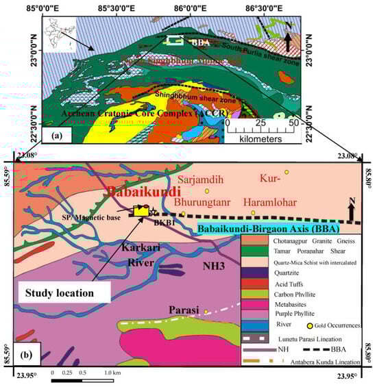
Figure 1.
Geological map of (a) Singhbhum Crustal Province and (b) the NSMB showing the Babaikundi–Birgaon Axis (BBA) and position of the study location with borehole location of BKB1.
The present work studies auriferous/sulfide zones within Babaikundi using the Scanning Electron Microscope (SEM), Backscattered-Electron (BSE), Magnetic, VLF-EM, and SP methods. Magnetic data were analyzed using upward continuation, Euler depth solution, radially averaged power spectrum, and analytical signal techniques. VLF-EM data were analyzed with a Fraser filter of the in-phase and out-phase components, a K–H plot of the in-phase component, and the inversion of VLF-EM data to obtain 2D resistivity sections. SP data were modeled using Particle Swarm Optimization (PSO), Very Fast Simulated Annealing (VFSA), and Genetic Algorithm (GA) inversion techniques. Geophysical inversion is a technique to recover the subsurface distribution of physical properties from field-collected data. The inversion problem is nonlinear and must be solved iteratively using an initial model. The starting model can be chosen freely, but it is usually selected as an initial model that is close to the assumed final model to avoid the inversion getting stuck in local minima. The initial model is progressively adapted in an iterative process until a proper fit is achieved between the observed and calculated data [6,9,10].
2. Geological Setting
The Singhbhum crustal province is divided into the northern younger province, consisting of a Singhbhum Group metasedimentary sequence [17,18], and the southern, older Iron Ore Series (Banded Iron formations, BIFs). The 200 km long, E-W trending, metasedimentary sequence, also known as NSMB [16,19], is an arcuate belt exhibiting a complex interplay of tectonism and sedimentation. According to Misra and Johnson [20], and Mahato et al. [21], the belt witnessed several reactivation episodes during the Archean Era. The study area is located in the northern part of NSMB, covering a part of the Babaikundi–Birgaon Axis (Figure 1). The bedrock geology with quartz reef is exposed in some areas, whereas most is assumed to be buried under a regolith soil layer [16]. Gold/sulfide (orogenic) mineralization is mainly distributed among the area’s sheared quartz veins and reefs. Hematite, pyrrhotite, magnetite, pyrite, and chalcopyrite are common minerals often associated with gold mineralization. The lithology of the study area comprises metasedimentary and metavolcanic rocks such as quartz–muscovite–sericite schist, quartzite, phyllite, limonitic quartzite, amphibolite, and ultramafic rocks [19]. Evidence of shearing is observed throughout the field and hand specimens such as s-c fabric, boudinages, and elongated quartz veins. Concentric rings of goethite, sericite, and martite indicate chemical alteration in the area [16]. Multiple generations of quartz veins occurring throughout the lithology emphasize the hydrothermal reworking of the area. The hydrothermal deposition of gold shows extensive variations in the geological environment, and its existence ranges from thin quartz veins to disseminated anomalies.
3. Methodology
Initially, the petrography studies (10 quartz samples) carried out using SEM-BSE images to understand the surficial occurrence of gold/sulfide minerals. Subsequently, a combined geophysical approach comprising magnetic, VLF-EM, and SP methods was used for the delineation of potential subsurface gold prospects/mineralization followed by an attempt to map the location of the Babaikundi–Birgaon Axis (BBA). The data were collected across the E-W trending luminiferous quartz reef exposure within the study area (Figure 2). The bedrock geology is outcropped in some areas, whereas most is buried under a regolith soil layer.
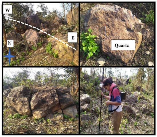
Figure 2.
Photographs of the ground surface and the east–west exposed outcrops in the study area.
Geophysical methods cannot directly detect the gold/sulfide minerals in the quartz vein; instead, they could map the probable locations and extension of the mineralized host rock—in this case, the subsurface quartz reef. A few mineral deposit types have elevated magnetizations due to the abundance of Fe-oxide and sulfide minerals (mainly magnetite). However, in most cases, magnetic responses provide (only) indirect information about deposits by indicating lineaments, intrusions, or defining different lithologies [22,23]. The SP method was primarily used to locate sulfide ore bodies by their electrochemical mechanisms [24] and oxidation potential [25]. Later, the SP method was used in geophysical applications, such as mineral exploration, geothermal exploration, hydrological investigation, environmental, and engineering applications [7,9,10,26,27,28]. The very low-frequency (VLF) electromagnetic (EM) method is the simplest EM method for delineating shallow subsurface conducting structures. It uses a single-user operating system to collect field data easily and rapidly. Detailed descriptions of the three methods can be found in Philips [29], Irvine and Smith [30], and Telford [31].
3.1. Magnetic Method
A total of 380 magnetic data readings were collected at 5 m intervals along six magnetic profiles, where each profile had a length of approximately 450 m. A Proton Precision Magnetometer (PPM) measured the total magnetic field with 0.01 nanoTesla (nT) sensitivity. Initially, magnetic data were corrected using diurnal correction. To remove the diurnal effects, a base station was selected some distance from the expected anomaly, and the base station reading was repeated with the same instrument after an interval of 30 min. The International Geomagnetic Reference Field (IGRF) was subtracted from field-observed data to find the final local magnetic anomaly. The data were gridded using the minimum curvature technique to produce a total magnetic intensity (TMI) anomaly map [32,33,34]. The TMI anomaly is the sum of low-frequency signals (generated mainly from deep-seated sources) and high-frequency signals (generated from shallow-seated sources) [30,31]. The 3D Euler deconvolution was carried out on IGRF-corrected magnetic data, and the corresponding depth solutions were plotted on the TMI map with different window sizes and depth tolerances. In general, 3D Euler deconvolution analysis is performed on magnetic data to estimate the depth and geometry, which is more an assumption made to obtain unambiguous depth estimates [35,36,37]. The method is based on Euler’s homogeneity equation, which is given as
where (xₒ, yₒ, zₒ) are the unknowns of the causative source, T is the magnetic-potential anomaly at a point (x, y, z), and N is the structural index. The structural index defines the assumed shape of the body causing an anomaly, where SI = 3 indicates a sphere, SI = 2 indicates a vertical or horizontal cylinder, and SI = 1 is associated with a thin sheet edge [36].
Upward continuation estimates the magnetic field at a higher elevation, highlighting the anomalies of longer spatial wavelengths [38]. The analytic signal or the total gradient method emphasizes the edges of the anomalous source body. Its great advantage is its independence of the magnetism direction of the original source. This removes any issues associated with remnant magnetism and avoids complications associated with small field inclinations at low-latitude magnetic responses [39]. Radial averaged power spectrum (RAPS) is a frequency domain technique to calculate the interface depth of the causative body [40,41,42].
RAPS can be expressed mathematically as
where p(k) is denoted as the power spectrum, k is the wavenumber, d is a mean depth estimate, and A is a constant.
By taking log on both sides of the equation:
Plotting ln(p) against the wavenumber k and fitting a straight line, the slope of that line denoted by can be used to estimate source depths. The slopes determined at the higher and lower wavelengths provide depth estimates at shallower and deeper points, respectively. Oasis Montaj, Geosoft software was used for magnetic data analysis.
3.2. Very Low-Frequency (VLF) Electromagnetic (EM) Method
The VLF data were acquired at a frequency of 18.6 kHz using the Portable GSM-19V instrument of GEM systems, Canada. The data were collected at a 5 m station interval along four profiles, A–A/, B–B/, C–C/, and D–D/, covering profile lengths of 470 m, 370 m, 450 m, and 300 m, respectively.
VLF surveying involves the measurement of the secondary magnetic field generated by the subsurface conducting bodies due to a primary electromagnetic signal generated by the transmitter at a great distance. Initially, the VLF was used in military navigation with a submarine radio transmitter designed for communication. The worldwide transmitters are located in coastal regions with a frequency band of 5–30 kHz, thus providing a freely available primary signal worldwide.
The VLF-EM method uses the electromagnetic (EM) induction phenomenon. According to Faraday’s law of EM induction, an electromotive force (EMF) is generated in a subsurface conductor, which sets up an eddy current in the subsurface conductor. This induced eddy current creates a secondary field, which propagates through the subsurface and is recorded at the receiver [42,43,44,45,46]. The VLF-EM method is a tilt angle method [42,43,44]. The generation of the elliptical shape of polarization around the subsurface conductor is due to the interaction between primary and secondary fields [46,47]. During acquisition, in-phase and out-phase components describing secondary magnetic fields are measured. For small secondary field strength, the real and imaginary components of Hz/Hx can be used to determine the tilt angle and presentation of the ellipticity, respectively [48]. Here, Hx (=Hp + Hxs) denotes the horizontal component of the primary field (Hp) and the horizontal component of the secondary field (Hxs), while Hz (=Hzs) is the vertical component of the secondary field. Tilt angle and ellipticity can be expressed as follows:
where Hx and Hz are the amplitude of magnetic fields representing horizontal and vertical components, respectively; is the phase difference denoted by , in which ϕz is the phase of Hz and ϕx is the phase of Hx; and . Fraser Filter (FF) is a linear filtering technique that converts the tilt angle by 90 degrees to indicate the conducting body, which leads to the crossover into peaks. Mathematically, FF can be written as [44]:
where F(0) are the filtered data, and , , etc., are measured data at successive stations. Karous and Hjelt’s (K–H) filtering technique is performed on real and imaginary components to obtain a 2D pseudo-current-density cross-section of the subsurface. The K–H filtering technique creates an equivalent current density against the subsurface conductor, producing a magnetic field identical to the measured field [49,50]. The coefficients of the K–H filter are multiplied with equispaced and consecutive observation points and summed up to give the corresponding current density value in the middle of those observation points. The real anomaly can only be considered enough to set up pseudo-current-density sections when the results of both real and imaginary components are almost the same [26]. However, the generated equivalent current density cross-section represents a pseudo section that is not the actual current distribution. The higher the current density value achieved from the K–H filtering, the greater the tendency to conduct within the subsurface.
3.3. Self-Potential (SP) Method
The SP technique broadly measures the naturally occurring potential differences due to electrochemical, electrokinetic, and thermoelectric fields in the Earth’s subsurface [7,25,51]. The SP data were acquired along four 520–550 m long profiles separated by ∼100 m distances. A high-input impedance digital multimeter (Fluke 287/289) with two non-polarizable Pb-Pb-Cl2 electrodes was used for SP data measurement. Data were collected with the total field method technique using a fixed base with a data point distance increment of 10 m [9]. The base station location was selected to be away from the expected anomaly but at a suitable point for the measurement. Repetitions of base station readings were carried out after each 30-min interval for drift correction. A small hole at each station was dug to remove the dry surface soil; hence, stable readings could be acquired during acquisition. The magnitude of the measured SP data varied within 4 to 6 mV. Further drift correction was applied to the acquired SP data, and the final drift-corrected SP anomaly data of profiles were used for SP inversion [6,9,10,52].
3.4. Inversion of SP Data
The SP anomaly V(x) expressed at any point R, for a sphere and cylinder [53,54], is given by
In Equation (7), k is the electric dipole moment or polarization magnitude, θ is the polarization angle, z is the depth, q is the shape factor, and x0 is the x coordinate of the center of the body. The shape factor q is sensitive to source geometry, which is 1.5 for spheres, 1.0 for horizontal cylinders, and 0.5 for vertical cylinders. In the present study, a shape factor of 1.0 was assumed because the sulfide-associated gold mineralization is considered to be of hydrothermal origin, which moves vertically upward and is deposited parallel to the Earth’s surface, which possibly acts as a cylindrical body.
3.4.1. Particle Swarm Optimization (PSO) Algorithm
PSO is a global optimization method initially introduced in 1995 by Kennedy and Eberhart [55]. It was used primarily to invert geophysical signals and self-potential datasets [56,57]. The processing steps involved in the PSO inversion are initializing the swarm, finding the local and global best values, local and global acceleration, choosing inertia weights, and repeating the cycle until the threshold number of iterations is reached. PSO is a population-based algorithm developed from the intelligence of swarms searching for food. The food source is based on the movement of individual birds or fish within the swarm. It may also be understood differently, considering the N individuals (particles) searching for the exit door in a room (search space). Initially, each individual is scattered and randomly positioned in the room, having an individual velocity, and this velocity controls the particle’s movement. An individual’s velocity depends on their current position and the best position achieved among the community in the room. The most reliable solution can be found in the PSO algorithm with the help of each individual. The primary purpose of the algorithm is to help each individual reach an exit door that is the required global minima. The global minima are accomplished by sharing the best fitness value by each individual and iteratively moving towards it. This can be formulated as follows:
Primarily, the initial position and velocities are assigned to the ith particle, denoted as Xi0 and Vi 0. At (k+1)th iteration, the velocities and positions are upgraded for the ith particle, as defined by Equations (9) and (10):
Here, Sk is defined as the global best fitness value until the kth iteration; Ri k is the best fitness value particle i; bl and bg are defined as cognitive and social scaling factors, respectively; and r1 and r2 are random numbers ranging between 0 and 1. Equation (9) is redefined by including the inertia weight term and given by Equation (11) as
The parameters (w, b1, bg) in Equation (8) have different values (0.8, 1.8, 2.0) [58], (0.6, 1.7, 1.7) [59], and (0.729, 1.494, 1.494) [60]. The selection of the parameters mainly depends on the nature of the inverse problem to be solved. We used (2.0, 2.0, 0.9) for the parameters (w, bl, bg) in the present study, respectively. The objective function (Q) is defined by Equation (9), which minimizes the difference between observed Vi0 and calculated Vic SP anomalies.
The equation computing the misfit error between the observed and calculated anomalies is expressed as follows:
3.4.2. Very Fast Simulated Annealing (VFSA) Algorithm
The Simulated Annealing (SA) algorithm is based on global minima [6,8,61,62] and was invented by Kirkpatric et al. [63]. The principle of SA is based on the slow cooling of melted metals after heating to crystallize their structures [61,62,64]. A newer and faster version of SA was named Very Fast Simulated Annealing (VFSA), which claimed fast convergence and resolved the problem of the slowness of SA. The important ability of VFSA is to escape the local minima and reach the global minima, which is achieved by selecting a neighbor randomly instead of choosing the best neighbor (best move) among possible neighbors in each stage of the algorithm. If the new state reduces the cost and makes it better, it is accepted as the next state, whereas if it increases the cost, it is accepted just with a probability of P (Metropolis probability) defined as
where the change in energy (generally caused by the difference in the state) that is the value of the cost function is denoted by , and T is the temperature that manages this probability. The initial parameter taken for VFSA is high temperature, called initial temperature. The number of attempts is accepted for each temperature until the system reaches a stable temperature state. Then, T’s value is decreased depending on an annealing process until it reaches zero or a very low temperature. The annealing process of VFSA depends on the Markov phenomenon carried out at constant temperature. Reducing the annealing temperature, i.e., the decreasing temperature being sufficiently slow, leads VFSA towards a global optimum with one probability. However, the fast decrease in temperature stops the algorithm’s movement and may stack on a local minimum.
3.4.3. Genetic Algorithm (GA)
The Genetic Algorithm (GA) is a random-based classical evolutionary algorithm that makes random changes to the current solution to generate a new solution. The theory of GA is established based on Darwin’s theory of evolution [65,66]. It shows biological evolution and random selection of the solution. It shows slight and slow changes to its solution until the best solution is achieved. Initially, GA works with the population; each consists of possible solutions to the given problem. Each solution is called an individual, represented by a set of genes (binary representation 0 and 1) equivalent to chromosomes. The fitness value is assigned to each individual to achieve the best individual in the solution. The fitness function represents the quality of the chromosome; the higher the fitness value, the higher the solution quality. In biology, a chromosome is known as a genotype, and the solution to the problem is represented as a phenotype. The selection of the best individual leads to the generation of a mating pool where the selected individuals are known as parents. Every two parents selected from the mating pool produce two offspring called children. Selecting and mating high-quality individuals will give the best optimal solution to the problem. A genetic algorithm involves three types of reproduction operators: selection, crossover, and mutation. The selection procedure is such that the probability of an individual being selected is proportional to that individual’s fitness. The selection of the number of individuals from the population is based on the individual fitness value. The model/target body and its parameters are updated biologically by coding the individual parameters as binary strings. The coding and decoding of the parameters are carried out using the following pair of equations:
where pib is a binary representation of the ith parameter and is the decimal representation of the ith parameter; represents the lower limit of the search space; denotes the search space of the corresponding parameter; and dec2bin and bin2dec are two operators used to convert decimal numbers to base-2 and vice versa, respectively. The misfit function is calculated using Equation (13): the fewer the misfit values, the greater the chance of obtaining global minima.
4. Results and Discussions
4.1. Petrography and Ore Mineralogy
The major rock units constituting this region are quartz-mica schist, phyllites, quartzites, carbonaceous phyllites, and high Mg-bearing basalts. The litho-unit of the area is intruded by quartz veins of three generations. The quartz veins are classified into three categories based on their morphology and mineral associations. Representative samples were collected from the study area to understand the host rocks’ texture, chemical, and mineralogical characteristics. Alteration patterns are common in the rocks of the region. The hydrothermal fluids are responsible for these alterations; hence, the alteration patterns are near the gold and sulfide mineralization. Figure 3 represents the photomicrograph of quartz samples: panels (a) and (b) indicate evidence of shearing with the presence of alternately arranged coarse- and fine-grained quartz (Qtz); (c) is a photomicrograph of quartz mica schist exhibiting S-C fabric; (d) shows the effect of sericitization and chloritization within metavolcanic rocks; (e) shows silicification within the metavolcanic rocks, which are associated with mineralization; (f) presents a photomicrograph of ultramafic rock; (g) shows a photomicrograph of pyrite grains in a quartz reef under cross-polarized light; and (h) denotes pyrite (Py) grains under reflected light. Mineralization in the area is associated with quartz veins intruding the meta–volcano–sedimentary and metavolcanic rocks. Pyrite, magnetite, chalcopyrite, pyrrhotite, arsenopyrite, hematite, and gold are common minerals associated with quartz veins in the area (Figure 4). Figure 4 presents the photomicrographs under reflected light and SEM-BSE images: (a) represents magnetite (Mag) getting altered to hematite (Hem), indicating an oxidizing environment; (b) shows alteration of hematite to goethite, showing the effect of leaching; (c) shows gold (Au) grains in reef quartz under reflected light—here, gold crystallizes at the crystal boundary; (d) indicates pyrrhotite (Po), sphalerite (Sp), and chalcopyrite (Ccp); (e) represents the alteration of magnetite to goethite (Gt); and (f) shows gold grains within quartz (Qtz). This study indicates that mineralization is hosted mainly by the quartz veins occurring at the contact margin of the quartz mica-schist and metavolcanic rocks. The sulfide- and oxide-bearing fluids show high prospects for gold. This Au-Cu sulfide ore mineralization is predominantly associated with magnetite and hematite. It is closely related to the complex structural deformation of the shear zone and lower-order brittle–ductile fracture zones.
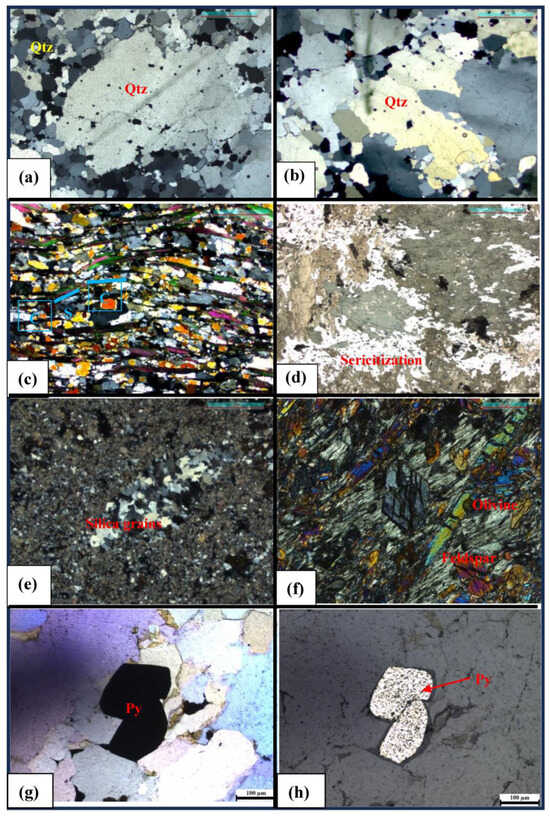
Figure 3.
(a,b) Photomicrographs of quartz samples showing evidence of shearing with the presence of alternately arranged coarse- and fine-grained quartz (Qtz). (c) Photomicrograph of quartz mica schist exhibiting S-C fabric. (d) Effect of sericitization and chloritization within metavolcanic rocks. (e) Silicification within the metavolcanic rocks, which is associated with mineralization. (f) Photomicrograph of ultramafic rock. (g) Photomicrograph of pyrite grains in quartz reef under cross-polarized light. (h) Pyrite (Py) grains under reflected light.
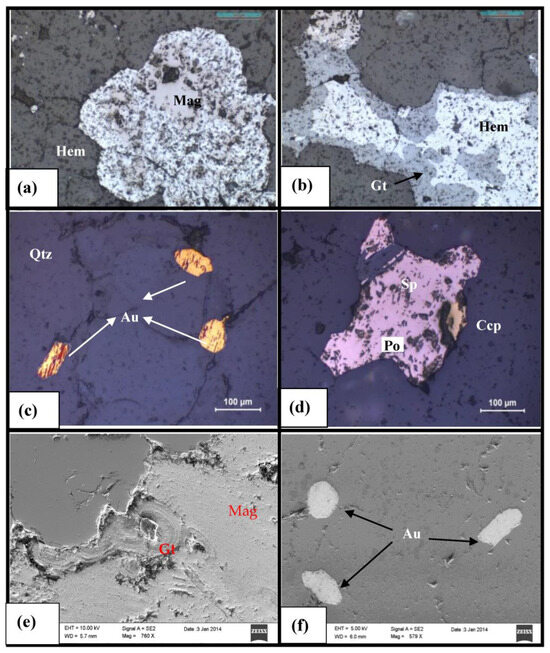
Figure 4.
Photomicrographs under reflected light and SEM-BSE images. (a) Magnetite (Mag) getting altered to hematite (Hem), indicating oxidizing environment. (b) Alteration of hematite to goethite, showing the effect of leaching. (c) Gold (Au) grains in reef quartz under reflected light—here, gold crystallizes at the crystal boundary. (d) Pyrrhotite (Po), sphalerite (Sp), and chalcopyrite (Ccp). (e) Alteration of magnetite to goethite (Gt). (f) Gold grains within quartz (Qtz).
4.2. Magnetic Method
The IGRF-corrected total magnetic intensity (TMI) anomaly map exhibits some high (~−503 to 352 nT) and low (~−1654 to −857 nT) anomalies (Figure 5). Low magnetic values (BML1, BML2, BML3, and BML4) are associated with demagnetization of magnetic properties due to hydrothermal alteration and are possibly considered as mineralized zones [30].
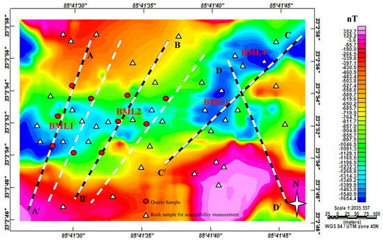
Figure 5.
Total magnetic intensity (TMI) map generated by six profile lines of magnetic data denoted by white dotted lines. SP and VLF-EM data were collected along four profiles: A–A/, B–B/, C–C/, and D–D/, marked by black–white lines.
Thirty-eight (38) rock samples were collected (locations shown in Figure 5; including locations of quartz sample for petrography) from outcrops in different parts of the study area for magnetic susceptibility measurement (Figure 6; Table 1). Susceptibilities were measured using a MPP-EM2S+ Multi-Parameter Probe. The magnetic susceptibility of the rock samples covering the shear zone indicates low susceptibility of about 0.49 × 10⁻⁶ to 60 × 10−6 SI, and the rock samples covering nearby parts of the shear zones demonstrate moderate susceptibility of about 60 × 10−6 to 100 × 10−6 SI. Similarly, the rock samples collected from other parts of the study area indicate relatively high susceptibility of about 100 × 10−6 to 180 × 10−6 SI.
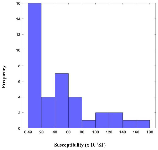
Figure 6.
Histogram plot of susceptibility of rock samples collected in Babaikundi.

Table 1.
Magnetic susceptibility range of rock samples collected in Babaikundi.
Three-dimensional Euler deconvolution was carried out for SI = 1, 2, 3 to estimate the solutions’ possible source geometry and clustering patterns. Figure 7 shows good clustering of the depth solutions with different colors on the map considering SI = 2, with a window size of 10 × 10 pixel square and depth tolerance of 10%, indicating a general geometry of a horizontal cylinder for the mineralized zone. The histogram of Euler depth solutions covering the study area shows that most solutions fall between 15 m and 35 m (Figure 8).
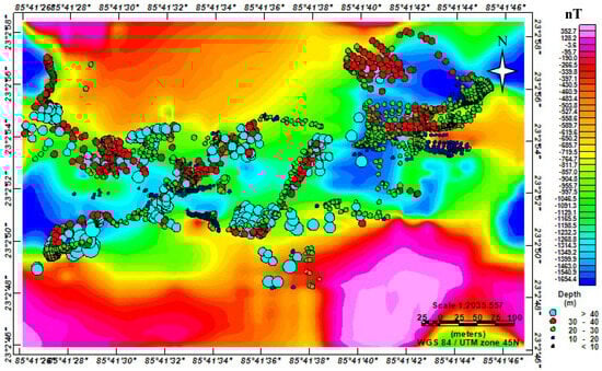
Figure 7.
Euler depth solution plot showing approximate depth to anomalies for SI = 2 using a squared window size of 10 × 10 pixels and depth tolerance of 10%. Euler depth solutions are superimposed over the TMI map.
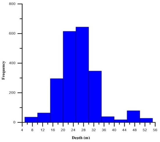
Figure 8.
Histogram of Euler depth solution for SI = 2 with window size of 10 × 10 pixel square and depth tolerance of 10%.
Upward continuations of the magnetic TMI data at 30 m and 60 m heights above the surface were carried out to remove possible high-frequency noises and understand deeper causative source trends (Figure 9 and Figure 10). Upward continuation of the magnetic TMI data at 30 m height (Figure 9) demarcates the shear zone with low magnetic anomalies from BMUL1, BMUL2, and BMUL3. As the continuation height increases, the effect of shallower features disappears [38]. Figure 10 reveals that the anomalies become smoother as the continuation height increases from 30 m to 60 m. The specified continuation height at 60 m signifies the region’s regional anomaly field (BMUL1 and BMUL2) from a depth below 30 m. Generally, upward-continued data exhibit responses from sources at depth > half the continuation height—this is a rule of thumb and applies only to layered sources [37]. The upward continuations of magnetic anomaly (Figure 9 and Figure 10) demonstrate the possible east–west shear zone extension with a prominent low magnetic anomaly value. The upward continuation map of 60 m (Figure 10) reveals the profoundly altered zone at a greater depth with a magnetic continued value of −1090.0 to −814.0 nT, signifying a prominent shear zone (BBA) in the area (Figure 10).
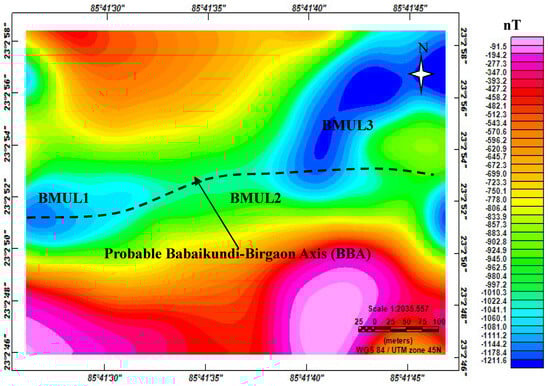
Figure 9.
Upward continuation (30 m) anomaly map shows the possible extension of the Babaikundi–Birgaon Axis (BBA) with the low magnetic anomaly (BMUL1, BMUL2, BMUL3).
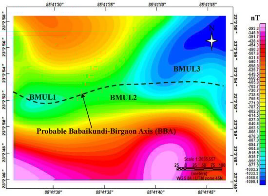
Figure 10.
Upward continuation (60 m) anomaly map shows the possible extension of the Babaikundi–Birgaon Axis (BBA) with a prominent and enhanced low magnetic anomaly boundary (BMUL1, BMUL2, BML3).
The maximum value of the analytical signal indicates the center with the highest depth of the possible mineralized body [67]. The analytical signal of the magnetic data is shown in Figure 11. The analytical signal of the magnetic data demonstrates two main anomalous zones, BAH1 and BAH2, ranging from ~21 to 59 nT, signifying a possible shear zone (BBA) in the area (Figure 11).
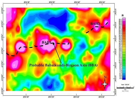
Figure 11.
Analytical signal map from the TMI anomaly in Babaikundi. Dashed lines BAH1 and BAH2 signify a possible shear zone (BBA).
The radially averaged power spectrum (RAPS) technique was used to calculate the depth of interfaces of different layers (Figure 12). Two prominent interfaces were identified with abrupt changes in magnetic value at about 40 m (deep-seated body) and about 25 m (shallow-seated body). The depth obtained from the RAPS analysis corroborates with the Euler depth solutions of magnetic data (Figure 8).
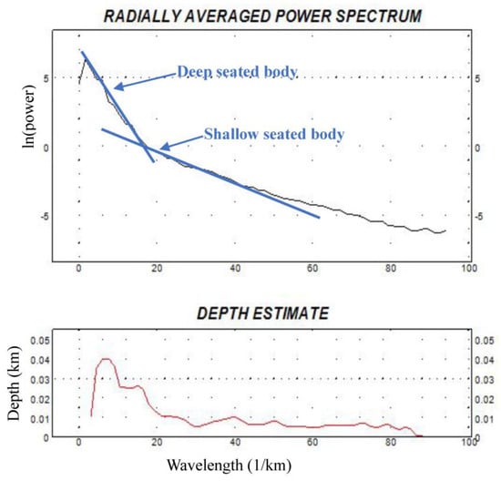
Figure 12.
Radially averaged power spectrum of the TMI map of the study area.
4.3. Very Low-Frequency (VLF) Electromagnetic (EM) Method
The VLF-EM data were filtered using the empirical mode decomposition (EMD) technique (EMTOMO, VLF2DMF-v1.6) to remove non-stationary noise and enhance the signal. The EMD filter decomposes the data into a finite number of intrinsic mode functions (IMFs) [68].
Figure 13a shows a plot of EMD-filtered data of A–A/, which shows a crossover of the real and imaginary VLF-EM data with zero axes at a reduced distance (RD) of ~230 m, indicating the possible location of an anomalous conducting feature/sulfide/gold body. The Fraser filter was applied on both in-phase and out-phase components, which shifts both components into a positive peak by 90 degrees at the same RD of ~230 m, indicating the subsurface conducting target (Figure 13b). The Karous–Hjelt (K–H) filter produces a 2D pseudo section of apparent current density, indicating a possible mineralized zone (AKZ1) with a high apparent current density value ranging from ~1.5 to 2.7% (Figure 13c). The VLF-EM data were inverted using the VLF2DMF program (EMTOMO) to generate an inverted 2D resistivity section [45,69,70,71]. The inverted 2D resistivity section demonstrates a low resistivity zone of ~ 50 Ωm, corresponding to the crossover of Figure 13a, with a root mean square (RMS) error of 0.4 (Figure 13d), indicating a possible mineralized zone (AKZ1) covering an RD of ~200 to 240 m at a depth of ~10 m to 45 m (Figure 13e).
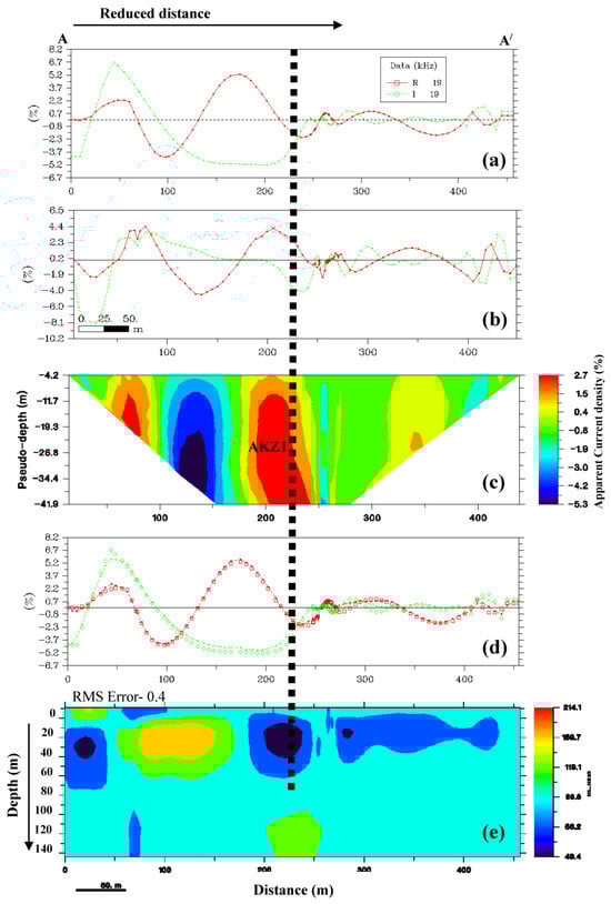
Figure 13.
VLF-EM data outputs along profile A–A/. (a) EMD-filtered plot with in-phase and out-phase components. (b) Fraser filter plot of in-phase and out-phase components. (c) K–H plot of in-phase components. (d) Data and model response curve. (e) 2D resistivity section after inversion of VLF-EM data. The black dotted line indicates the location of the anomalous conducting zone.
Profile B–B/ shows the EMD-filtered data (Figure 14a) with a crossover point at an RD of ~170 m, while the Fraser filter plot also shows the positive peak for the corresponding reducing distance (Figure 14b). The K–H pseudo section presents a high current density of ~10%–14.5% (Figure 14c) corresponding to the crossover point (Figure 14a,b), illustrating a conducting zone possibly associated with sulfide/gold mineralization. The inverted 2D resistivity section of profile B–B/ with RMS error 0.3 demonstrates a low resistivity value of ~1–40 Ωm covering an RD of ~130 to 180 m at a depth of ~10 to 40 m (Figure 14e), possibly indicating a zone of sulfide/gold mineralization (Figure 14d).
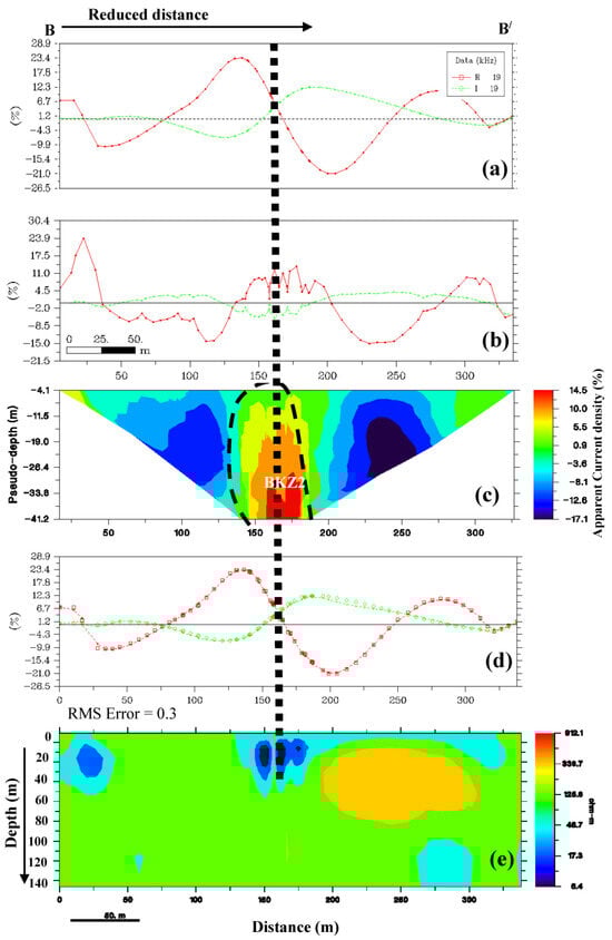
Figure 14.
VLF data outputs along profile B–B/. (a) EMD-filtered plot with in-phase and out-phase components. (b) Fraser filter plot of in-phase and out-phase components. (c) K–H plot of in-phase component. (d) Data and model response curve. (e) 2D resistivity section after inversion of VLF-EM data. Black dotted line indicates the location of the anomalous conducting zone.
For profile C–C/, the crossover point is located at an RD of ~225 m (Figure 15a); the Fraser filter plot also indicates a positive peak at the same RD (Figure 15b), while the K–H plot shows a current density of ~10%–12.8% (Figure 15c). The inverted 2D resistivity section (Figure 15e) with an RMS error of 0.1 (Figure 15d) gives the low resistivity (~10–30 Ωm) value covering RD ~150 to 280 m at a depth of ~1 to 40 m for the location corresponding to a crossover point and positive peak at the RD of ~225 m.
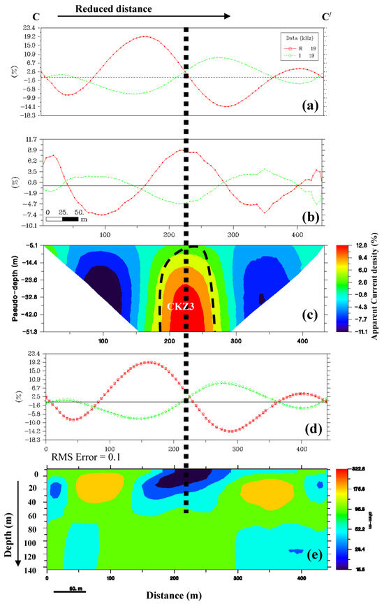
Figure 15.
VLF data outputs along profile C–C/. (a) EMD-filtered plot with in-phase and out-phase components. (b) Fraser filter plot of in-phase and out-phase components. (c) K–H plot of in-phase components. (d) Data and model response curve. (e) 2D resistivity section after inversion of VLF-EM data. Black dotted line indicates the location of the anomalous conducting zone.
The profile D–D/ reveals the crossover point at an RD of ~110 m (Figure 16a), corresponding to a positive peak after applying the Fraser filter (Figure 16b), indicating a pseudo current density of ~4.4 to 8.2% (Figure 16c). The inverted 2D section of profile D–D/ with the RMS value of 0.2 (Figure 16d) demonstrates a low resistivity value of ~4 to 20 Ωm covering an RD of ~100 to 135 m at a depth of ~10 to 40 m (Figure 16e), possibly indicating an anomaly related to the mineralized body. Additional low-resistivity zones observed in Figure 13, Figure 14, Figure 15 and Figure 16 possibly indicate incorrect results because they are neither correlated with the crossover between the real and imaginary component of VLF-EM data nor with the high current density value that is essential to be considered as an anomalous conducting feature.
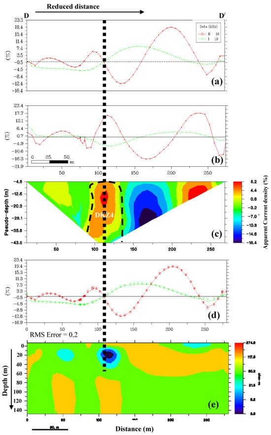
Figure 16.
VLF data outputs along profile D–D/. (a) EMD-filtered plot with in-phase and out-phase components. (b) Fraser filter plot of in-phase and out-phase components. (c) K–H plot of in-phase components. (d) Data and model response curve. (e) 2D resistivity section after inversion of VLF-EM data. Black dotted line indicates the location of the anomalous conducting zone.
Further, the Fraser-filtered in-phase data were generated separately from all the profiles A–A/, B–B/, C–C/, and D–D/ using VLF2DMF software. All generated data were compiled to prepare a grid map [72,73,74], which shows the four prominent anomalies, BF1, BF2, BF3, and BF4, with a high Fraser-filtered in-phase value of ~2.1%–4.1%. The locations of the four profiles, A–A/, B–B/, C–C/, and D–D/, of SP and VLF-EM are mentioned on the map (Figure 17).
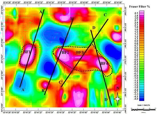
Figure 17.
Fraser-filtered map of the in-phase component of profiles A–A/, B–B/, C–C/, and D–D/ in the study area. BF1, BF2, BF3, and BF4 represent zones of high Fraser-filtered in-phase value. The locations of four profiles, A–A/, B–B/, C–C/, and D–D/, of SP and VLF-EM are shown on the map.
Similarly, the K–H in-phase data of the four profiles, A–A/, B–B/, C–C/, and D–D/, were also generated using VLF2DMF software to prepare a grid map to locate the high current density location [72,73,74,75]. The KH map shows the high current density value ranging from ~2.2 to 8%, delineated by BKH1, BKH2, BKH3, and BKH4 (Figure 18). The zones of high current density values were generated due to the presence of the secondary field, possibly indicating anomalous sulfide/gold-bearing mineralized zones in the subsurface.
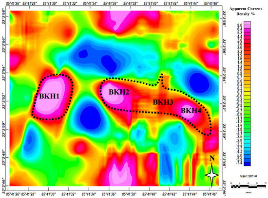
Figure 18.
K–H map of the in-phase component of profiles A–A/, B–B/, C–C/, and D–D/ in the study area. BKH1, BKH2, BKH3, and BKH4 represent zones of high current density.
4.4. Results of SP Inversion
SP inversion was performed in four profiles, A–A/, B–B/, C–C/, and D–D/, using PSO, VFSA, and GA inversion techniques.
4.4.1. Particle Swarm Optimization (PSO) Algorithm
The initial parameters used for the inversion of drift-corrected SP data using the PSO algorithm [76] are listed in Table 2a. The results after the inversion are tabulated in Table 2b. The inverted results suggest that the depth of the anomalous body is between 20 and 30 m. The low misfit in all four profiles implies that the origin of the body is acceptable.
Table 2.
(a): The input parameters used for PSO inversion of corrected SP data. (b): Interpreted SP model parameters using PSO for gold associated with sulfide ore deposits in Babaikundi.
4.4.2. Very Fast Simulated Annealing (VFSA) Algorithm
The drift-corrected SP data were inverted using the VFSA algorithm considering the initial model parameter given in Table 3a. The VFSA-based inversion results for each profile are summarized in Table 3b. In general, it is found that the depth range of the anomalous body varies from 18 m to 35 m.
Table 3.
(a): The input parameters used for VFSA inversion of corrected SP data. (b): Inverted SP model parameters estimated using VFSA.
4.4.3. Genetic Algorithm (GA)
The initial parameters—i.e., population size = 200, mutation rate = 0.6, and selection rate = 0.5 [66]—were used in the GA. The evolutionary process runs for several iterations until the minimum misfit is achieved. The initial and inverted output model parameters are tabulated in Table 4a and Table 4b, respectively.
Table 4.
(a): The input parameters used for GA inversion of corrected SP data. (b): Inverted SP model parameters estimated using GA.
4.4.4. Comparisons of Inverted SP Models Based on PSO, VFSA, and GA Algorithms
A detailed comparison of the inverted model parameters obtained using PSO, VFSA, and GA algorithms for profiles A–A/, B–B/, C–C/, and D–D/ is shown in Table 5 (Figure 19). The approximate depth of the anomaly is found to lie within ~ 20 to 30 m, with the RD ranging between ~160 and 212 m, having a misfit error percentage of 0.0010–0.0018 using the PSO algorithm. The VFSA-based inverted model, with a misfit of ~0.001%–0.0039%, indicates the depth of the target anomaly at ~18 to 35 m, with the RD ranging between ~172 and 205 m. The GA-based inverted model, with a misfit of ~3%–4.4%, shows that the depth of the anomalous body lies between ~23 and 37 m, with the RD ranging between ~173 and 208 m.
Table 5.
Comparison among PSO, VFSA, and GA based on quantitative data: depth (z), distance (x˳), and misfit of the inverted model.
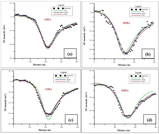
Figure 19.
SP plots of field data and modeled data estimated using PSO, VFSA, and GA algorithms for profiles (a) A–A/. (b) B–B/, (c) C–C/, and (d) D–D/.
The above results reveal that the PSO algorithm offers the best-fitted model parameters of the causative body that corroborate well with the approximate depth estimated using 3D Euler deconvolution and RAPS analysis of magnetic data.
5. Conclusions
A combined analysis of SEM-BSE images, magnetic data, VLF-EM data, and SP data was carried out for the possible existence of BBA and the occurrence of gold-bearing sulfide minerals in quartz reef (Figure 20). The combined study of photomicrography with low-magnetic anomaly at a depth of ~25 to 40 m, high current density/low resistivity at a depth of ~1 to 40 m according to VLF-EM, and negative SP anomaly at a depth of ~20 to 30 m indicate the existence of the BBA and the occurrences of gold-bearing auriferous sulfide minerals in the limonitic quartz reef.
Important findings from the present study are as follows:
- The study of photomicrographs under reflected/transmitted light and SEM-BSE images reveals the presence of gold in the quartz reef along with pyrrhotite, sphalerite, and chalcopyrite.
- The photomicrographs of quartz samples provide evidence of shear/fracture with alternate coarse and fine quartz grains.
- The magnetic survey reveals that mineralized areas fall within fracture zones with low magnetic anomaly values.
- The Euler depth solution of magnetic data indicates that the favorable depth of the causative bodies lies between 15 m and 35 m, which corroborates with the 25 to 40 m depth derived using RAPS of the magnetic data.

Figure 20.
(a) Map showing study area (Babaikundi) across the Babaikundi–Birgaon Axis (BBA). (b) Photomicrographs under reflected light and SEM-BSE images of the collected samples in Babaikundi. (c1) Upward continued (60 m) magnetic anomaly map showing possible extension of a part of BBA. (c2) RAPS of total magnetic intensity map showing magnetic value at about 40 m (deep-seated body) and about 25 m (shallow-seated body). (d) VLF-EM data outputs along profile C–C/ showing mineralized zone covering reduced distance (RD) of ~150 to 280 m at a depth of ~ 1 to 40 m. (e) SP plots of field data and inverted model data produced from GA, VFSA, and PSO algorithms for profile C–C/ at a depth of ~29 to 30 m and RD ~208–212 m.

- The VLF-EM analysis proposes the sulfide/gold mineralization in the depth range of ~1 to 40 m (Borehole BKB-1).
- The quantitative analysis of PSO, VFSA, and GA indicates that PSO provides a more suitable target depth and location with minimal misfit.
- A comprehensive study of magnetic, SP, and VLF-EM data delineates the possible extension of BBA with a depth of the auriferous sulfide minerals ranging between 3 and 40 m that corroborates with Borehole BKB-1.
Author Contributions
D.H.: Data curation, Formal analysis, Methodology and Writing draft; S.K.P. and S.S.: Conceptualization, Validation, Resources, Final writing, Supervision; A.B.: Methodology, Software, Formal analysis. All authors have read and agreed to the published version of the manuscript.
Funding
Department of Science and Technology, Government of India for funding project nos. SB/S4/ES-640/2012, FST/ES-I/2017/12, and DST/TDT/SHRI-16/2021(C&G); ISRO, Government of India: ISRO/RES/630/2016-17; Ministry of Coal, Government of India: No. CMPDI/B&PRO/MT-173.
Data Availability Statement
Datasets analyzed during the current study are available from the corresponding author upon reasonable request.
Acknowledgments
We are grateful to the editors and the reviewers for their constructive comments on this paper for further improvements. We would also like to thank, IIT (ISM), Dhanbad, for providing all basic facilities in this study.
Conflicts of Interest
The authors declare that they have no known competing financial interests or personal relationships that could have appeared to influence the work reported in this paper.
References
- Grooves, D.I.; Phillips, G.N. The Genesis and Tectonic Control on the Archaean Gold Deposits of the Western Austrian Shield: A Metamorphic replacement Model. Ore Geol. Rev. 1987, 2, 287–322. [Google Scholar] [CrossRef]
- Colvine, A.C. An Empirical Model for the Formation of Archaean Gold Deposits; Final Products of Cratonization of the Superior Province, Canada. Econ. Geol. Monogr. 1989, 6, 37–53. [Google Scholar]
- Madhusudan, I.C.; Maiti, S.K.; De, M.K.; Singh, A.; Das, P.C. Geophysical studies of Tamar Gold Prospect, Babaikundi-Birgaon Sector, District Ranchi, Bihar. Ind. Min. 1999, 53, 37–44. [Google Scholar]
- Macnae, J.C. Kimberlites and exploration geophysics. Geophysics 1979, 44, 1395–1416. [Google Scholar] [CrossRef]
- Smith, R.J. Geophysics of Iron Oxide Copper-Gold Deposits Hydrothermal Iron Oxide Copper–Gold and Related Deposits: A Global Perspective. PGC Publ. 2002, 2, 357–367. [Google Scholar]
- Biswas, A.; Sharma, S.P. Optimization of Self-Potential interpretation of 2-D inclined sheet-type structures based on Very Fast Simulated Annealing and analysis of ambiguity. J. Appl. Geophys. 2014, 105, 235–247. [Google Scholar] [CrossRef]
- Biswas, A.; Sharma, S.P. Interpretation of self-potential anomaly over idealized body and analysis of ambiguity using very fast simulated annealing global optimization. Near Surf. Geophys. 2015, 13, 179–195. [Google Scholar] [CrossRef]
- Biswas, A. A comparative performance of Least Square method and Very Fast Simulated Annealing Global Optimization method for interpretation of Self-Potential anomaly over 2-D inclined sheet type structure. J. Geol. Soc. India 2016, 88, 493–502. [Google Scholar] [CrossRef]
- Horo, D.; Pal, S.; Singh, S.; Srivastava, S. Combined self-potential, electrical resistivity tomography and induced polarisation for mapping of gold prospective zones over a part of Babaikundi-Birgaon Axis, North Singhbhum Mobile Belt, India. Explor. Geophys. 2020, 51, 507–522. [Google Scholar] [CrossRef]
- Horo, D.; Pal, S.; Singh, S. Mapping of Gold Mineralization in Ichadih, North Singhbhum Mobile Belt, India Using Electrical Resistivity Tomography and Self-Potential Methods. Min. Metall. Explor. 2021, 38, 397–411. [Google Scholar] [CrossRef]
- Vacquier, V.; Holmes, C.R.; Kintzinger, P.R.; Lavergne, M. Prospecting for Groundwater by Induced Electrical Polarisation. Geophysics 1957, 23, 660–687. [Google Scholar] [CrossRef]
- Klein, J.D.; Sill, W.R. Electrical properties of artificial clay bearing sandstone. Geophysics 1982, 47, 1593–1605. [Google Scholar] [CrossRef]
- Towel, J.N.; Anderson, R.G.; Pelton, W.H.; Olhoeft, G.R.; LaBrecque, D. Direct Detection of Hydrocarbon Contaminants using Induced Polarisation Method: SEG Meeting. In Proceedings of the 1985 SEG Annual Meeting, Washington, DC, USA, 6–10 October 1985; pp. 145–147. [Google Scholar]
- Sesha Sai, V.V. A Report on Exploration for Gold in Babaikundi-Birgaon Sector, District Ranchi; Unpublished Program Report of GSI F.S. 1995–1996; Geological Survey of India: Bihar, India, 1998.
- Maiti, S.K.; De, M.K.; Singh, A.; Das, P.C. A Report on Geophysical Studies of the Babaikundi-Birgaon Sector, Tamar Gold Prospect, District Ranchi, Bihar (F.S. 1997–1998); Geological Survey of India: Bihar, India, 1999.
- Jha, V.; Singh, S.; Venkatesh, A.S. Invisible gold occurrences within the quartz reef of Babaikundi area, North Singhbhum fold-and-thrust belt, Eastern Indian Shield: Evidence from petrographic, SEM and EPMA studies. Ore Geol. Rev. 2015, 65, 426–432. [Google Scholar] [CrossRef]
- Sarkar, S.N.; Saha, A.K. A revision of Precambrian stratigraphy and tectonics of Singhbhum and adjacent regions. Q. J. Geol. Min. Metall. Soc. India 1962, 34, 97–136. [Google Scholar]
- Saha, A.K. Crustal evolution of Singhbhum-North Orissa, Eastern India. Mem. Geol. Soc. Ind. 1994, 27, 341. [Google Scholar]
- Chandan, K.K.; Jha, V.; Roy, S.; Khatun, M.; Sahoo, P.R.; Singh, S. Ore microscopic study of the gold mineralisation within Chandil Formation, North Singhbhum Mobile Belt, Eastern India. Int. J. Earth Sci. Eng. 2014, 6, 213–222. [Google Scholar]
- Misra, S.; Johnson, P.T. Geochronological Constraints on Evolution of Singhbhum Mobile Belt and Associated Basic Volcanics of Eastern Indian Shield. Gondwana Res. 2005, 8, 129–142. [Google Scholar] [CrossRef]
- Mahato, S.; Goon, S.; Bhattacharya, A.; Mishra, B.; Bernhardt, H.-J. Thermo-tectonic evolution of the North Singhbhum Mobile Belt (eastern India): A view from the western part of the belt. Precambrian Res. 2008, 162, 102–127. [Google Scholar] [CrossRef]
- Park, J.O.; You, Y.J.; Kim, H.J. Electrical resistivity surveys for gold-bearing veins in the Yongjang mine, Korea. J. Geophys. Eng. 2009, 6, 73–81. [Google Scholar] [CrossRef]
- Fon, A.N.; Bih Che, V.; Emmanuel Suh, C. Application of Electrical Resistivity and Chargeability Data on a GIS Platform in Delineating Auriferous Structures in a Deeply Weathered Lateritic Terrain, Eastern Cameroon. Int. J. Geosci. 2012, 3, 960–971. [Google Scholar] [CrossRef]
- Sato, M.; Mooney, H.M. The electrochemical mechanism of sulfide self–potentials. Geophysics 1960, 25, 226–249. [Google Scholar] [CrossRef]
- Corry, C.E. Spontaneous polarisation associated with porphyry sulphide mineralisation. Geophysics 1985, 50, 1020–1034. [Google Scholar] [CrossRef]
- Sharma, S.P.; Baranwal, V.C. Delineation of groundwater bearing fracture zones in a hard rock area integrating very low frequency electromagnetic and resistivity data. J. Appl. Geophys. 2005, 57, 155–166. [Google Scholar] [CrossRef]
- Mehanee, A.S. Tracing of paleo-shear zones by self-potential data inversion: Case studies from the KTB, Rittsteig, and Grossensees graphite-bearing fault planes. Earth Planets Space 2015, 67, 14–47. [Google Scholar] [CrossRef]
- Kumar, S.; Pal, S.K. Underground coalfire mapping using analysis of self-potential (SP) data collected from Akashkinaree Colliery, Jharia coalfield, India. J. Geol. Soc. India 2020, 95, 350–358. [Google Scholar] [CrossRef]
- Phillips, W.J.; Richards, W.E. A study of the effectiveness of the VLF method for the location of narrow-mineralized fault zones. Geoexploration 1975, 13, 215–226. [Google Scholar] [CrossRef]
- Irvine, R.J.; Smith, M.J. Geophysical exploration for epithermal gold deposits. J. Geochem. Explor. 1990, 36, 375–412. [Google Scholar] [CrossRef]
- Telford, W.M.; Geldart, L.P.; Sheriff, R.E. Applied Geophysics; Cambridge University Press: Cambridge, UK, 1990. [Google Scholar]
- Guo, W.W.; Li, Z.X.; Dentith, M.C. Magnetic petrophysical results from the Hamersley Basin and their implications for interpretation of magnetic surveys. Aust. J. Earth Sci. 2011, 58, 317–333. [Google Scholar] [CrossRef]
- Holden, E.J.; Wong, J.C.; Kovesi, P.; Wedge, D.; Dentith, M.; Bagas, L. Identifying structural complexity in aeromagnetic data: An image analysis approach to greenfields gold exploration. Ore Geol. Rev. 2012, 46, 47–59. [Google Scholar] [CrossRef]
- Kumar, S.; Pal, S.; Guha, A.; Sahoo, S.D.; Mukherjee, A. New insights on Kimberlite emplacement around the Bundelkhand Craton using integrated satellite-based remote sensing, gravity and magnetic data. Geocarto Int. 2020, 37, 1–23. [Google Scholar] [CrossRef]
- Thompson, D.T. EULDPH—A new technique for making computer-assisted depth estimates from magnetic data. Geophysics 1982, 47, 31–37. [Google Scholar] [CrossRef]
- Reid, A.B.; Allsop, J.M.; Granser, H.; Millet, A.J.; Somerton, I.W. Magnetic interpretation in three dimensions using Euler deconvolution. Geophysics 1990, 55, 80–91. [Google Scholar] [CrossRef]
- Agarwal, B.N.P.; Srivastava, S. Analyses of self-potential anomalies by conventional and extended Euler deconvolution techniques. Comput. Geosci. 2009, 35, 2231–2238. [Google Scholar] [CrossRef]
- Jacobsen, B.H. Case for upward continuation as a standard separation filter for potential-field maps. Geophysics 1987, 52, 1138–1148. [Google Scholar] [CrossRef]
- Rajagopalan, S. Analytic Signal vs. Reduction to Pole: Solutions for Low Magnetic Latitudes. ASEG Ext. Abst. 2003, 2, 1–4. [Google Scholar] [CrossRef]
- Spector, A.; Grant, F.S. Statistical models for interpreting aeromagnetic data. Geophysics 1970, 35, 293–302. [Google Scholar] [CrossRef]
- Blakely, R.J. Potential Theory in Gravity and Magnetic Applications; Cambridge University Press: Cambridge, UK, 1995. [Google Scholar]
- Mishra, D.C. Gravity and Magnetic Methods for Geological Studies; BS Publications: Hyderabad, India, 2011. [Google Scholar]
- Alexopoulos, J.; Vassilakis, E.; Dilalos, S. Combined geophysical techniques for detailed groundwater flow investigation in tectonically deformed fractured rocks. Ann. Geophys. 2013, 56, S0669. [Google Scholar] [CrossRef]
- Sharma, S.P.; Biswas, A.; Baranwal, V.C. Very low frequency electromagnetic method: A shallow subsurface investigation technique for geophysical applications. In Recent Trends in Modelling of Environmental Contaminants; Springer: Berlin, Germany, 2014; pp. 119–141. [Google Scholar]
- Baranwal, V.C.; Franke, A.; Borner, R.U.; Spitzer, K. Unstructured grid based 2-D inversion of VLF data for models including topography. J. Appl. Geophys. 2011, 75, 363–372. [Google Scholar] [CrossRef]
- Baranwal, V.C.; Sharma, S.P. Integrated geophysical studies in the East-Indian geothermal province. Pure Appl. Geophys. 2006, 163, 209–227. [Google Scholar] [CrossRef]
- Parasnis, D. Mining Geophysics, Methods in Geochemistry and Geophysics; Elsevier: Amsterdam, The Netherlands, 1973. [Google Scholar]
- Paterson, N.R.; Ronka, V. Five Years of Surveying with the Very Low Frequency-Electromagnetic Method. Geoexploration 1971, 9, 7–26. [Google Scholar] [CrossRef]
- Karous, M. Effect of relief in EM methods with very distant source. Geoexploration 1979, 17, 33–42. [Google Scholar] [CrossRef]
- Karous, M.; Hjelt, S.E. Linear filtering of VLF dip-angle measurements. Geophys. Prospect. 1983, 31, 782–794. [Google Scholar] [CrossRef]
- Revil, A.; Jardani, A. The Self-Potential Method: Theory and Applications in Environmental Geosciences; Cambridge University Press: Cambridge, UK, 2013. [Google Scholar]
- Srivardhan, V.; Pal, S.K.; Vaish, J.; Kumar, S.; Bharti, A.K.; Priyam, P. Particle swarm optimisation inversion of self-potential data for depth estimation of coal fires over East Basuria colliery, Jharia coalfield, India. Environ. Earth Sci. 2016, 75, 688. [Google Scholar] [CrossRef]
- Yungul, S. Interpretation of spontaneous polarization anomalies caused by spheroidal ore bodies. Geophysics 1950, 15, 237–246. [Google Scholar] [CrossRef]
- Bhattacharya, B.B.; Roy, N. A note on the use of nomograms for self-potential anomalies. Geophys. Prospect. 1981, 29, 102–107. [Google Scholar] [CrossRef]
- Kennedy, J.; Eberhart, R. Particle swarm optimization. In Proceedings of the ICNN’95-International Conference on Neural Networks, Perth, Australia, 27 November 1995. [Google Scholar]
- Peksen, E.; Yas, T.; Kayman, A.Y.; Özkan, C. Application of particle swarm optimization on self-potential data. J. Appl. Geophys. 2011, 75, 305–318. [Google Scholar] [CrossRef]
- Santos, F.A.M. Inversion of self-potential of idealized bodies using particle swarm optimization. Comput. Geosci. 2010, 36, 1185–1190. [Google Scholar] [CrossRef]
- Martínez, F.J.L.; Gonzalo, E.G.; Fernandez, P.; Kuzma, H.; Omar, C. PSO: A powerful algorithm to solve geophysical inverse problems: Application to a 1D-DC resistivity case. J. Appl. Geophys. 2010, 71, 13–25. [Google Scholar] [CrossRef]
- Trelea, I.C. The particle swarm optimization algorithim: Convergence analysis and parameter selection. Inf. Process. Lett. 2003, 85, 317–325. [Google Scholar] [CrossRef]
- Clerc, M.; Kennedy, J. The Particle Swarm: Explosion, Stability, and Convergence in a Multi-Dimensional Complex Space. IEEE Trans. Evol. Comput. 2002, 6, 58–73. [Google Scholar] [CrossRef]
- Ingber, L. Very fast simulated re-annealing. Math. Comput. Model. 1989, 12, 967–973. [Google Scholar] [CrossRef]
- Ingber, L. Simulated annealing: Practice versus theory. Math. Comput. Model. 1993, 18, 29–57. [Google Scholar] [CrossRef]
- Kirkpatrick, S.; Gelatt, C.D., Jr.; Vecchi, M.P. Optimization by Simulated Annealing. Science 1983, 220, 671–680. [Google Scholar] [CrossRef] [PubMed]
- Baghmisheh, M.T.V.; Navarbaf, A. A Modified Very Fast Simulated Annealing Algorithm. In Proceedings of the 2008 International Symposium on Telecommunications, Tehran, Iran, 27–28 August 2008. [Google Scholar] [CrossRef]
- Davis, L. Handbook of Genetic Algorithms; Van Nostrand Reinhold: New York, NY, USA, 1991. [Google Scholar]
- Eiben, A.E.; Smith, J.E. Introduction to Evolutionary Computing; Springer: Heidelberg, Germany, 2015. [Google Scholar]
- Elkhodary, S.T.; Youssef, M.A.S. Integrated potential field study on the subsurface structural characterization of the area North Bahariya Oasis, Western Desert, Egypt. Arab. J. Geosci. 2013, 6, 3185–3200. [Google Scholar] [CrossRef]
- Huang, N.E.; Wu, Z. A review on Hilbert–Huang transform: The method and its applications on geophysical studies. Rev. Geophys. 2008, 46, RG2006. [Google Scholar] [CrossRef]
- Beamish, D. Two-dimensional regularised inversion of VLF data. J. Appl. Geophys. 1994, 32, 357–374. [Google Scholar] [CrossRef]
- Beamish, D. Quantitative 2D VLF data interpretation. J. Appl. Geophys. 2000, 45, 33–47. [Google Scholar] [CrossRef]
- Kaikkonen, P.; Sharma, S.P. 2-D nonlinear joint inversion of VLF and VLF-R data using simulated annealing. J. Appl. Geophys. 1998, 39, 155–176. [Google Scholar] [CrossRef]
- Fraser, D.C. Contouring of VLF-EM data. Geophysics 1969, 34, 958–967. [Google Scholar] [CrossRef]
- Alexopoulos, J.D.; Dilalos, S.; Tsatsaris, A.; Mavroulis, S. ERT and VLF measurements contributing to the extended revelation of the ancient town of Trapezous (Peloponnesus, Greece). In Proceedings of the Near Surface Geoscience 2014—20th European Meeting of Environmental and Engineering Geophysics, Athens, Greece, 14–18 September 2014; pp. 1–5. [Google Scholar]
- Khalil, M.A.; Santos, F.A.M.; Moustafa, S.M.; Saad, U.M. Mapping water seepage from Lake Nasser, Egypt, using the VLF-EM method: A case study. J. Geophys. Eng. 2009, 6, 101. [Google Scholar] [CrossRef]
- Kumar, S.; Pal, S.K.; Guha, A. Very low Frequency electromagnetic (VLF-EM) study over Wajrakarur kimberlite Pipe 6 in Eastern Dharwar Craton, India. J. Earth Syst. Sci. 2020, 129, 102. [Google Scholar] [CrossRef]
- Kumar, R.; Pal, S.K.; Gupta, P.K. Water Seepage Mapping in an Underground Coal-Mine Barrier Using Self-potential and Electrical Resistivity Tomography. J. Mine Water Environ. 2020, 40, 622–638. [Google Scholar] [CrossRef]


Disclaimer/Publisher’s Note: The statements, opinions and data contained in all publications are solely those of the individual author(s) and contributor(s) and not of MDPI and/or the editor(s). MDPI and/or the editor(s) disclaim responsibility for any injury to people or property resulting from any ideas, methods, instructions or products referred to in the content. |
© 2023 by the authors. Licensee MDPI, Basel, Switzerland. This article is an open access article distributed under the terms and conditions of the Creative Commons Attribution (CC BY) license (https://creativecommons.org/licenses/by/4.0/).