Abstract
For the mineral exploration in complex terrain areas, the semi-airborne transient electromagnetic (SATEM) technology is one of the most powerful methods due to its high efficiency and low cost. However, since the mainstream SATEM systems only observe the component dBz/dt and the data are usually processed by simple interpretation or one-dimensional (1D) inversion, their resolutions are too low to accurately decipher the fine underground structures. To overcome these problems, we proposed a novel 3D forward and inversion method for the multi-component SATEM system. We applied unstructured tetrahedron grids to finely discretize the model with complex terrain, subsequently we used the vector finite element method to calculate the SATEM responses and sensitivity information, and finally we used the quasi-Newton method to achieve high-resolution underground structures. Numerical experiments showed that the 3D inversion could accurately recover the location and resistivities of the underground anomalous bodies under the complex terrain. Compared to a single component data, the inversion of the multi-component data was more accurate in describing the vertical boundary of the electrical structures, and preferable for high-resolution imaging of underground minerals.
1. Introduction
Geophysical methods are important tools for mineral resources exploration [1]. The conventional ground geophysical methods require humans to access and operate equipment, which is quite difficult and almost impossible for the work in dangerous mountain areas. In contrast, the airborne electromagnetic (AEM) technology can overcome the inaccessibility of terrain and achieve efficient and high-precision data to detect the underground structures [2]. However, the AEM technology generally requires a manned helicopter as a carrier, and the cost is too high. The semi-airborne transient electromagnetic (SATEM) method, also known as the ground-air transient EM method, uses the grounded electrical source or the loop source as a transmitter, and it uses the unmanned aerial vehicle (UAV) to carry the EM sensors as the receivers. This method not only has the advantages of large exploration depth of ground transient EM systems, but it can also achieve rapid exploration at a lower cost [3,4,5]. The SATEM method is one of the preferred tools for mineral explorations in mountain areas and other complex environments [6,7].
The SATEM method was first proposed by Nabighian [8] in 1988 as a geophysical exploration method. In the 1990s, Elliot developed the FLAIRTEM (Fixed Loop Airborne Transient Electromagnetic) system [9,10]. Elliot used a large loop source as a transmitter and successfully detected a sulfide ore deposit in Papua New Guinea [11]. Smith et al. [12] and Yang and Oldenburg [13] conducted experiments on the ground, including the use of SATEM and AEM systems in a sulfide mining area. Mogi et al. [14] developed the first SATEM system called GREATEM using light helicopters for data acquisition, and they used this system to investigate the geothermal field in the Beppu area of southwestern Japan. Subsequently, Ito et al. [15,16] used this system to conduct deep exploration in the Aso volcanic area of Japan. Ji et al. [17] carried out significant work on the theoretical research, the system development, the data processing, and the interpretations of the SATEM system. Recently, a German consortium, comprising the Federal Institute for Geosciences and Natural Resources (BGR), three universities, two research institutes and two companies, established the Deep Electromagnetic Sounding for Mineral Exploration (DESMEX) project [5,6,7] to develop a SATEM system. Kotowski et al. [3] evaluated the results of the system developed in the DESMEX project.
Compared to the rapid development of the SATEM equipment, the data processing and interpretation are still underdeveloped and mostly use conductivity-depth imaging [18] and 1D inversion [19]. Although these imaging and 1D inversions can deliver a rough image to the underground structures, they cannot as yet achieve accurate results for the SATEM data acquired in areas with complex terrain, where the mineral exploration is often desirable; thus there is a need to develop a more accurate and practical data interpretation technology [5,6,7]. Furthermore, although the SATEM method provides a good solution to the rapid acquisition of data to detect the underground electrical structures in complex terrain areas, it usually only measures the dBz/dt component, which is useful for detecting the horizontal conductive anomalies, but has low resolution for dipping and vertical anomalies, representing typical ore bodies and fracture zones, etc. Taking these problems into account, we present our study about the 3D forward and the inversion method under complex terrain conditions for the multi-component SATEM in this research.
At present, there are many numerical simulation methods that can be applied to the SATEM forward modeling, such as the integral equation (IE) method [20], the finite-difference (FD) method [21], the finite-volume (FV) method [22], and the finite-element (FE) method [23], etc. The IE, FD, and FV methods generally use a structured grid to discretize the model, as they have poor adaptability to complex models. In contrast, the unstructured tetrahedral grids are suitable for modeling complex terrain [24,25,26]. In this paper, we use the FE method for the simulation of the SATEM field under complex terrain. The commonly used 3D inversion methods are nonlinear conjugate gradient (NLCG) method [27]. This method avoids the calculation of Hessian matrix but requires multiple linear searches in each iteration to find the optimal step for model updates. The Gauss-Newton (GN) method uses both the information of the first and second derivatives of the objective function, having approximate quadratic convergence and number of required model updates is often less than NLCG [28,29] but this method requires too much time to compute the Hessian matrix. The Limited Memory quasi-Newton method (L-BFGS) [30] uses the gradient and correction of limited iterations to simplify the approximation to the Hessian matrix, and thus requires less memory and converges quickly. Therefore, in this research, we use the L-BFGS method to minimize the objective function for our inversion.
This paper focuses on the detection capability analysis of the multi-component SATEM using 3D forward modeling and inversions by considering complex terrain. We present our work in the following order: firstly, we introduce the basic theory of forward modelling and the inversion algorithm; subsequently, we show the accuracy and the response analysis of the simple plate model; finally, we test on an inclined ore body model with complex terrain and the Ovoid massive sulfide deposit to show the advantages of our method.
2. Method
2.1. Governing Equations
The Maxwell’s equations in time-domain can be written as [31]
Neglecting the displacement current in Equation (2), we can derive the diffusion equation for the electric field as [28]
where e(r,t) and h(r,t) are the electric and magnetic field at position r and time t, js is the imposed source current, while μ, ε, and σ are respectively the magnetic permeability, dielectric permittivity and conductivity.
2.2. Spatial and Time Discretization
We adapt the unstructured finite-element method [32] for our modeling, and discretize the computational domain into tetrahedral elements. In each element, the electric field can be expressed as,
where, Nik(r) and eik(t) are, respectively, the vector basis functions [33] and the electric field along the ith edge of the kth element.
From Equation (3), we can define a residual vector, i.e.,
and by assuming that the weighted residual integral of each element is zero, we have
where, Re is the residual vector of element e, v is the volume of element e. Taking Equation (5) into (6), we obtain
The (i,j) element of matrix A,B and the ith element of matrix S can be written as
For time discretization, we adopt unconditionally the stable backward Euler method [29,34,35]. The second order form can be obtained approximately by a Taylor expansion, i.e.,
Taking Equation (11) into (7), we obtain
2.3. Boundary Conditions and Source Term
To ensure that there is a unique solution to the EM field, we assume that the outer boundary of the simulation area is far enough away from the transmitting source, so the electric field satisfies the Dirichlet boundary condition [35], i.e.,
where, n is the normal vector of the outside boundary Γ of the calculation domain.
We consider that the SATEM method is generally based on electrical transmitting sources. Therefore, when the transmitting waveform is a step-up or pulse wave, the initial electric field is zero and when the transmitting waveform is a step-off wave, the initial electric field is the solution of a DC problem. The potential generated by the point source satisfies Poisson’s equation. The potential at the boundary meets the Dirichlet boundary condition, so the boundary value problem can be expressed as
where φ(r) is the potential at position r. We adopt the unstructured node-based FE method to solve the problem [34].
2.4. Forward Modeling Equation
Assembling Equation (12) for all time channels [28], we obtain the following equation:
where Cn = 3A+2ΔtnB, sn = 2ΔtnSn. Equation (16) can be rewritten as
where K is the coefficient matrix, e is the electric field, and ss is the source term. We adopt the direct solver MUMPS [36] to factorize Equation (12) to obtain the electric field at the edges of each tetrahedron element and obtain dBx,y,z/dt at the receiver location via Faraday’s law.
2.5. Regularized Inversion
For the geophysical 3D inversion, the number of model parameters is usually much larger than that of survey data. Mathematically, such problems are underdetermined problems. To overcome the non-unique solutions brought by the underdetermined problems, Tikhonov [37] proposed a regularization method, which reduces the multiple solutions by reducing the size of the solution space. Based on this, we propose the following objective function for 3D time-domain EM inversions, i.e.,
where, m denotes the parameter vector of the conductivity model, d is the Nd dimensional data vector, Cd is a diagonal matrix whose elements are composed of the covariance of the data error, while f(m) is the forward response calculated by the vector FE method. m0 is the initial model, λ is trade-off parameter, and Cm is the model roughness operator. By differentiating both sides of Equation (18) with respect to the model parameter m, we obtain the gradient of the objective function [28] as
where r = d f(mn), J represents the sensitivity matrix. In this paper, the BFGS method is used to search the step length to obtain the model update Δm, subsequently the new model is obtained by mn+1 = mn + Δm.
2.6. Sensitivity Matrix
To obtain the gradient of the objective function, we need to calculate the sensitivity matrix first. We use the adjoint forward method [28] to compute the sensitivity matrix implicitly. This method avoids directly storing the sensitivity matrix and thus can largely reduce the memory consumption. The sensitivity matrix J can be expressed as
where, L = LtLd. Ld is the interpolation operator that maps the electric field to the data locations, whereas Lt is used to interpolate data from the computational time channels to observed ones.
Differentiating both sides of Equation (17) with respect to model parameters, we obtain
then JTrd can be expressed as
Assuming that
we have
since A and C in Equation (16) are symmetric, KT can be written as
From Equation (25), a reverse recursive process is needed to solve the adjoint forward modeling of u. After the adjoint forward modeling, we substitute u into Equation (22) and obtain
To obtain the product of the transposed sensitivity matrix and the vector, we still needed to calculate (∂K/∂m)e and ∂SS/∂m. By referring to Equation (21), (∂K/∂m)e can be obtained by a simple calculation. For ∂SS/∂m, since we use the total field method for forward modeling, si in the source term is independent of the conductivity, so we have
When the direct method is used to solve the forward problem, we can save the decomposition results of matrix K, which can largely reduce the calculations by directly calling in the accompanying forward process. It must be pointed out that when the step-off wave is used for calculation, the initial electric field contains underground conductivity information, so another item ∂Ae0/∂m in Equations (16) and (17) needs special treatment. For this purpose, we write ∂Ae0/∂m as
where the term (∂A/∂m)e0 can be obtained by simple calculation, but A(∂e0/∂m) needs to be calculated by adjoint forward modeling in DC field simulation [28].
2.7. Model Roughness Constraint
We use the following model roughness for our 3D time-domain inversion [28]
where,
while, Vi is the volume of the ith element, Ni is the number of elements that share the nodes with the ith element, Δrij is the distance between the centroids of the current element and the jth adjacent element.
2.8. Termination Condition for the Inversion
In the inversion process, the root mean square (RMS) is used to judge whether to terminate an inversion that is defined by
where ei is the noise standard deviation of ith data. When the RMS drops to 1, we believe that the data has been well fitted and the inversion is terminated. However, when the inversion falls into a local minimum, the RMS cannot drop to 1. At that time, we use the gradient value to judge whether to terminate the inversion. The judgment conditions are defined as
where, ε is a small real number.
3. Numerical Experiments
In this section, we performed numerical experiments of forward modeling and inversions to analyze the ability of our newly proposed method. All the tests were performed on a workstation equipped with an Inter (R) Xeon (R) 3.1GHz CPU and 128 GB of memory.
3.1. Accuracy Verification
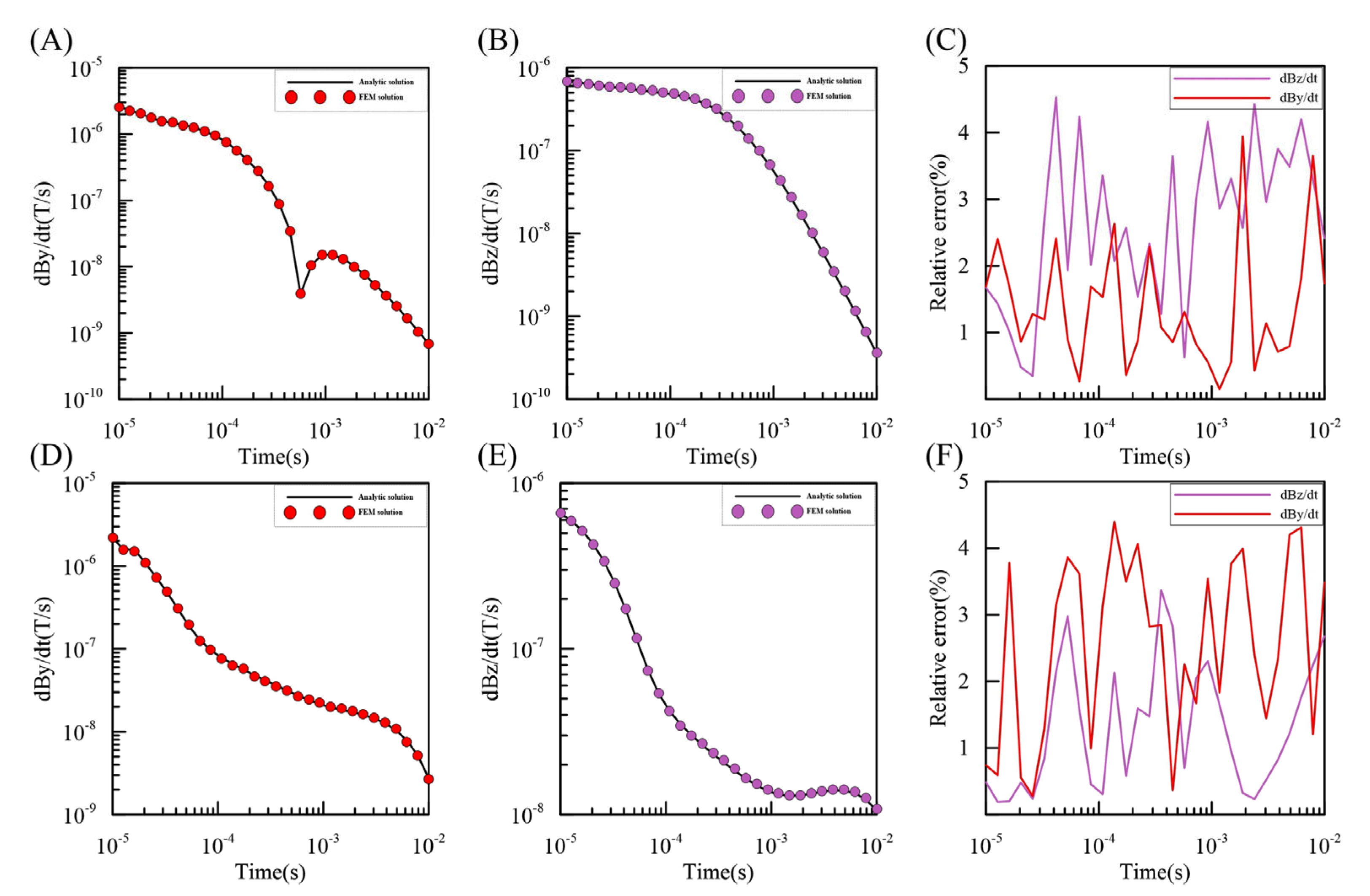
To verify the accuracy of our 3D time-domain FE method, we assumed a uniform half-space and a layered model to compare our 3D time-domain results with 1D semi-analytical solutions. We set up a Cartesian coordinate system with the horizontal surface at z = 0 m and z axis positive downwards. The uniform half-space had a resistivity of 100 Ω∙m and the H-type 1D model had three layers with the resistivity of 100 Ω∙m, 10 Ω∙m and 100 Ω∙m, respectively, and with the thickness of the first two layers being 50 m. An electrical transmitting source of 1000 m long was used as a source with the center located at (0 m, −500 m, 0 m). The transmitting current was 1 A and the waveform was a step-off wave. The receiver was in the air at (0 m, 0 m, −30 m). Figure 1 shows the comparison of the results. Since the transmitting source is parallel to the x-axis, the response in the x-direction of the receiving point is zero, consequently we only compared the EM field components in the other two directions. It can be seen that the 3D forward modeling results in this paper are in good agreement with 1D semi-analytical solutions, with the maximum relative error being less than 5%.
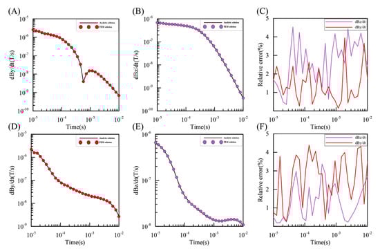
Figure 1.
Accuracy verification for the homogeneous and three-layer model. (A–C) are the dBy/dt, dBz/dt and relative error for the uniform half-space model; (D–F) are the dBy/dt, dBz/dt and relative error for the layered earth model.
3.2. Detectability Analysis of Multi-Component Responses for Plate Models
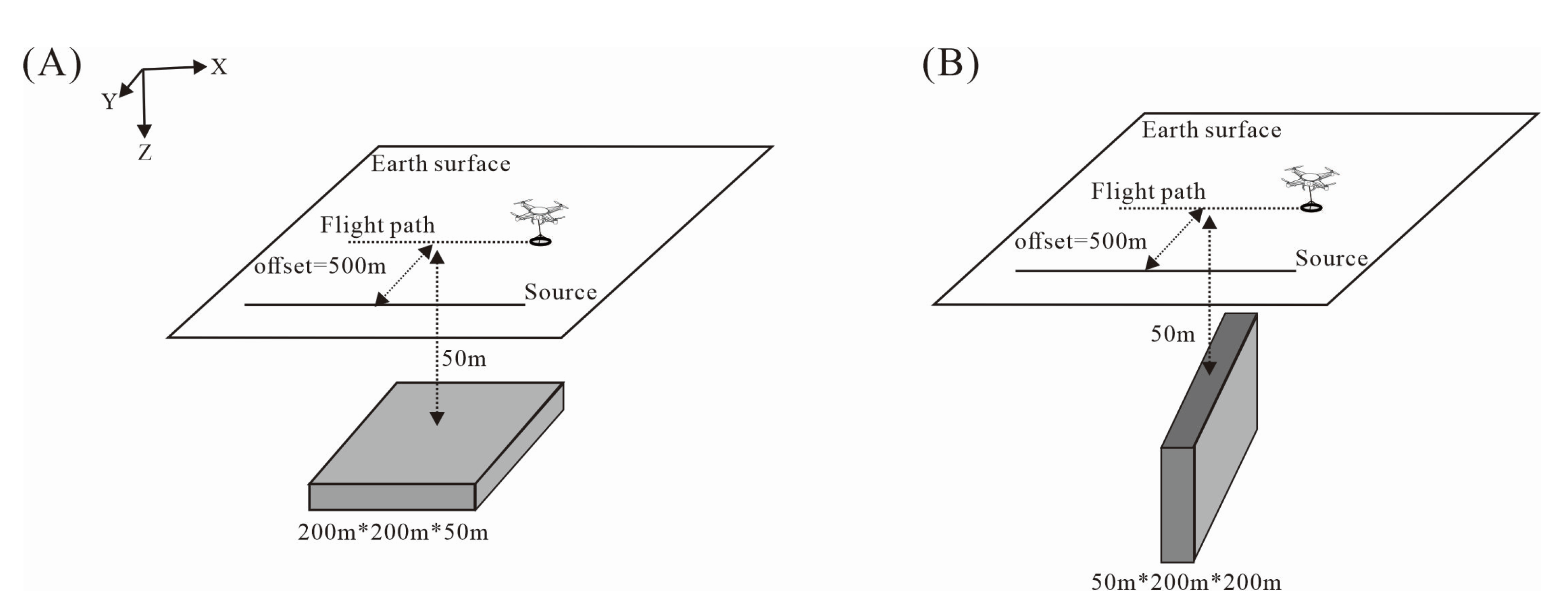
To analyze the detectability of each EM component for the anomalous body, we designed two models, one with a horizontal plate and the other with a vertical plate with resistivity of 1 Ω∙m, buried in a uniform half-space of 100 Ω∙m (Figure 2). The size of plates is 200 m × 200 m × 50 m and 50 m × 200 m × 200 m in horizontal and vertical plate models, respectively, and the depth of the top of the plate is 50 m in both the models. An electrical source parallel to the x-axis is used as the transmitter, with the center located at (0 m, −500 m, 0 m). The transmitting current is step-off wave of 50 A. The flight altitude is 30 m with offset between the transmitter and the receivers as 500 m. The survey line is 400 m long along the x-axis and the interval between surveying points is 25 m.
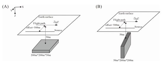
Figure 2.
Plate models (A) Horizontal plate; (B) Vertical plate.
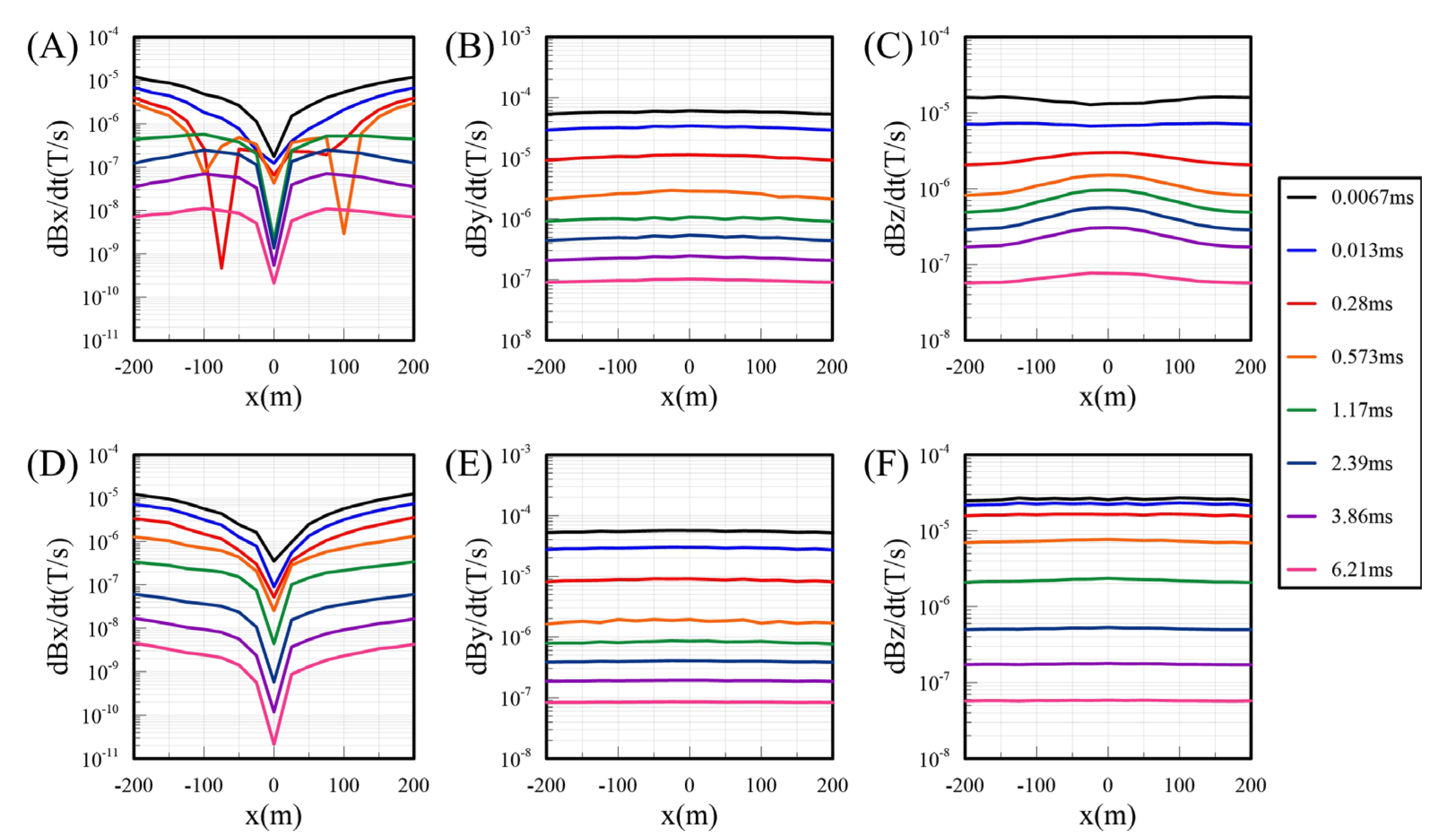
Figure 3 shows the multi-component responses for the two models in Figure 2. It can be seen that for the horizontal plate model, the EM responses in the x direction and z direction can both reflect the existence of the anomalous body, but dBx/dt can better reflect the locations of the vertical boundaries. For the vertical plate model, it is not possible to distinguish the anomalous body only by the response in the z direction, while dBx/dt can still clearly reflect its existence. Therefore, in practical applications, it is necessary to measure multi-component EM fields to better depict the anomalous bodies.
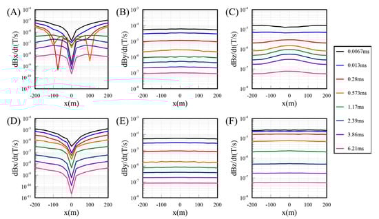
Figure 3.
EM responses for the plate models in Figure 2 at y = 0 m. (A–C) are the dBx/dt, dBy/dt and dBz/dt for the Horizontal plate model; (D–F) are the dBx/dt, dBy/dt and dBz/dt for the Vertical plate model.
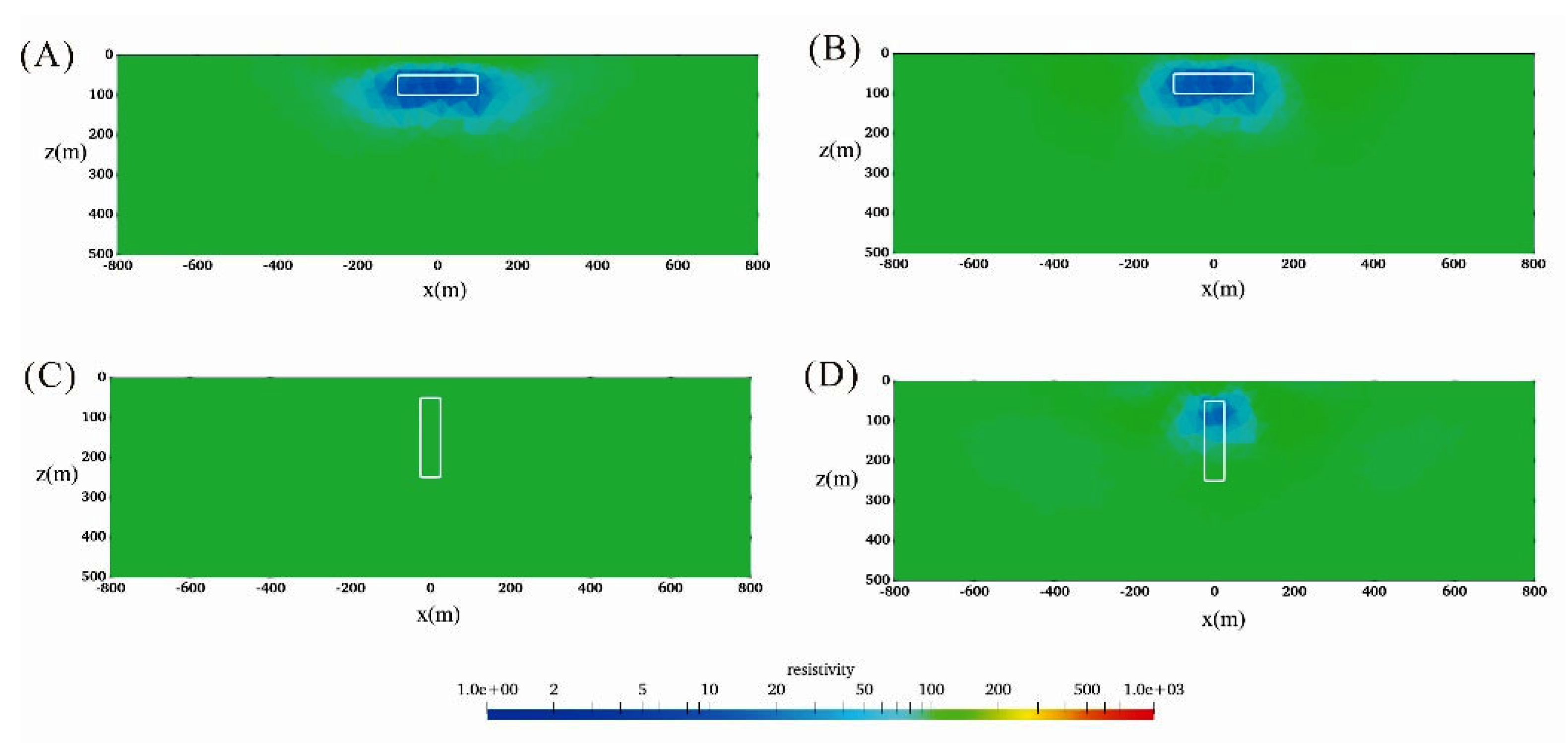
To verify the effectiveness of our inversion algorithm, we inverted forward modelled data from the plate models with 3% Gaussian noise to single component and multi-component data, respectively. Nine survey lines parallel to the x-axis were planned between −200 m and 200 m, with 50 m line spacing along the y-axis. There were 41 measurement points on each line, with 30 m flight altitude. The same transmitting source as shown in Figure 2 was used to generate the synthetic data. From Figure 4A,B, we can see that the single and the multi-component inversions can both recover the position and the resistivity of the anomalous body, but the multi-component inversion has more capability to depict the vertical boundaries of the plate (Figure 4B,D).
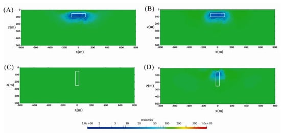
Figure 4.
3D Inversions of horizontal and vertical plate models sliced at y = 0 m. (A,C) are z component inversions of horizontal and vertical plate models, respectively, while (B,D) are multi-component inversions of horizontal and vertical plate models, respectively.
Figure 4C,D show the inversion results for the vertical plate model. It can be seen that for the vertical plate model, since the response of its vertical component can barely see the existence of the anomalous body (see Figure 3F), the inversion results from the vertical component alone cannot recover the anomalous body. In contrast, the multi-component inversion can better recover the location and resistivity of the anomalous vertical body though it fails to recover the correct depth of the bottom of the vertical body. This confirms that the horizontal components are very important in the detection of inclined structures.
3.3. Inclined Ore Body under Complex Terrain
Considering that the mineralization is often found in mountainous areas with complex terrain, the data interpretation and the inversion must consider the effect of the terrain. In this section, we designed an inclined ore body below an undulating terrain (Figure 5) to verify the practicability of our algorithm. The size of the ore body was 750 m × 300 m × 300 m and the depth of the center point of the ore body was 200 m below the horizontal surface. The resistivity of the ore body and background was 1 and 100 Ω∙m, respectively. For this inversion test, we designed 12 survey lines between 700 m and 1800 m in the x direction with a line spacing of 100 m. There were 61 survey points on each line at an interval of 25 m between 0 and 1500 m in the y direction with a flight altitude of 30 m. The transmitting source was 1 km long aligned in the y-axis direction with a 500 m offset to the nearest measurement point. Figure 5A,B show the locations of the source, survey points and the inclined ore body. Figure 5C,D show the grids used for forward modeling and inversions, respectively. The forward model was discretized into 642338 tetrahedral elements, and the inverse model was discretized into 608834 elements. All the synthetic data was contaminated by 3% Gaussian noise.
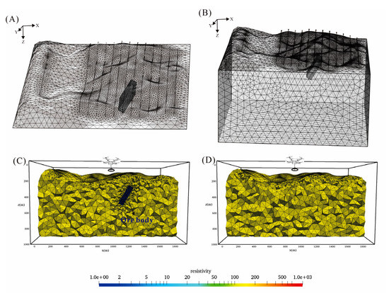
Figure 5.
Forward and inverse models for an inclined ore body model. (A,B) show the locations of the source, survey points and the inclined ore body, (C) is the discretization of the inclined model for forward modeling, (D) is the discretization of the model for inversion.
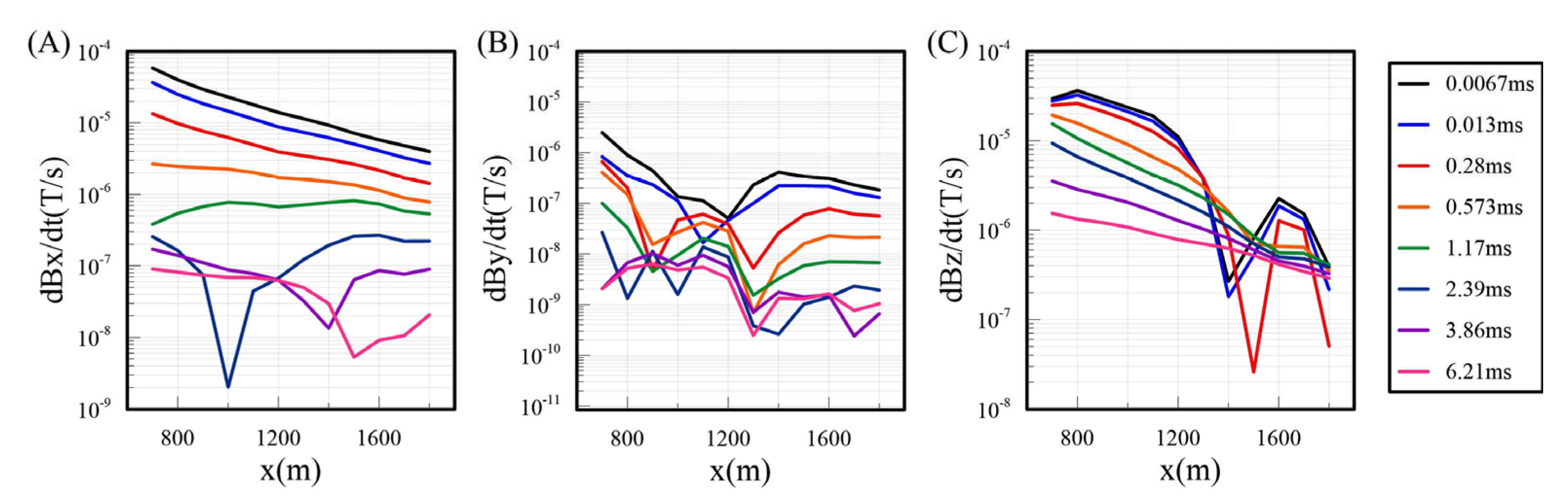
To analyze the characteristics of the response of the inclined ore body model, we displayed the response along the central surveying line passing over the ore body in Figure 6. Due to the existence of complex terrain, the response curves had obvious fluctuations in the early time channels. Since the transmitting source in this example was parallel to the y axis (different from that in Section 3.2), the component of dBy/dt was obviously affected by the anomaly body (see Figure 6B), so that it had the potential to improve the inversion result. We note that even under the influence of the terrain, the dBz/dt component was still sensitive to the steep anomaly body (Figure 6C), thus it could recover the inclined ore body to some extent.

Figure 6.
Multi-component responses of inclined ore body model at y = 700 m. (A–C) are the X component, Y component and Z component, respectively.
Figure 7 shows the inversion results for the inclined ore body model. It can be seen that the inversions of the vertical component alone could not well depict the horizontal location and extent of the anomalous body (Figure 7A), while the multi-component inversions could better recover the location, dipping nature and the resistivity of the target. This example shows the practicability of the multi-component inversions together with complex terrain.

Figure 7.
3D inversions of an inclined ore body model. (A,C) are vertical and horizontal clips at y = 750 m and z = 350 m of single-component inversion result for the inclined ore model respectively, while (B,D) are the corresponding clip of multi-component inversion results for the inclined ore model.
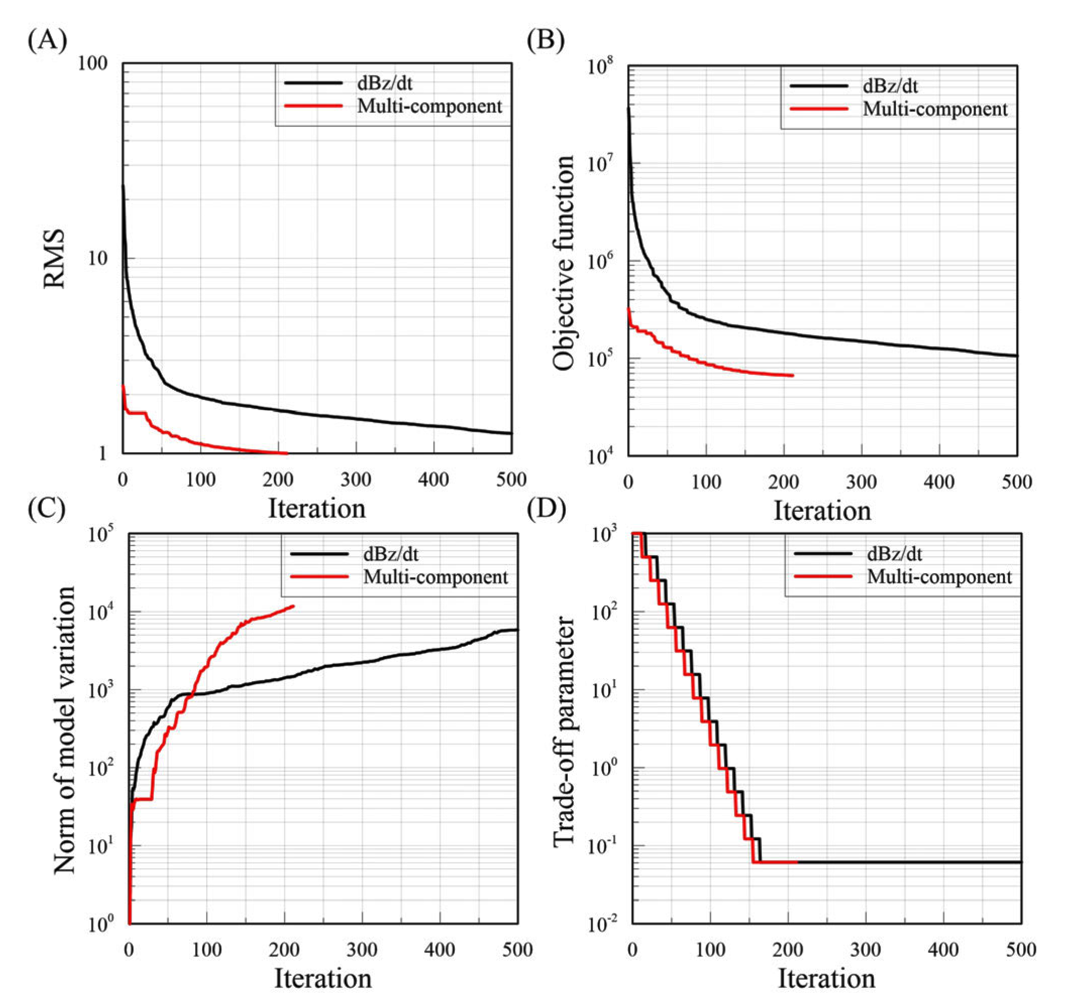
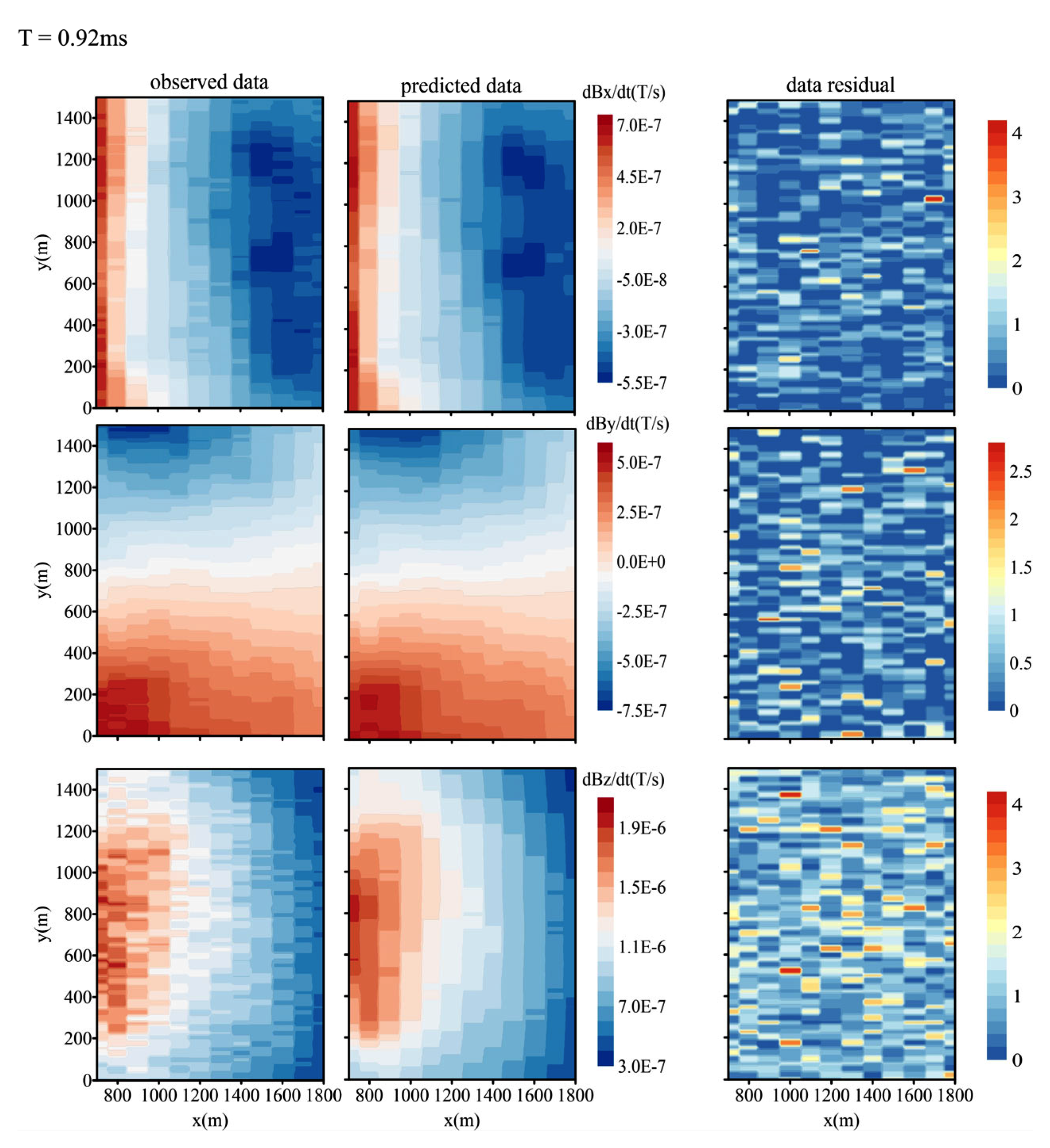
Figure 8 shows the parameters of the SATEM inversion for an inclined ore body through various iterations. It can be seen that the RMS and objective function values for the two inversions decreased rapidly at early stage. When the RMS approached 1, the model variations tended to be stable, which proved that the inversions worked well. Meanwhile, compared with the single component inversion, the multi-component inversions proposed in this paper needed fewer iterations to converge. Figure 9 shows the comparison between the noise-added synthetic data and the predicted data for the multi-component inversion at t = 0.92 ms for an inclined ore body. The distribution of each component of the predicted data was very similar to the observed ones, and the noise in the synthetic data was smoothed out. The RMS for most of the survey points was in the range between 0 and 2 (other than a few points which were greater than 2), which means that most of the data have been fitted well.
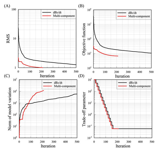
Figure 8.
Inversion parameter versus iterations for the inclined ore body model. (A) is the RMS (B) is the objective function (C) is the norm of model variation and (D) is the trade-off parameter.
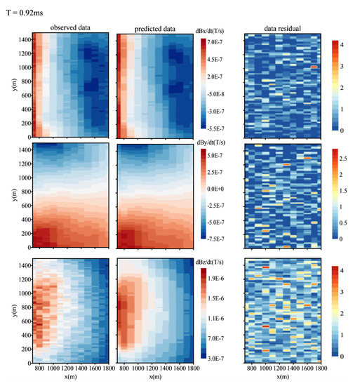
Figure 9.
Data fitting of multi-component inversion for the inclined ore body model.
3.4. Application to the Ovoid Massive Sulfide Deposit
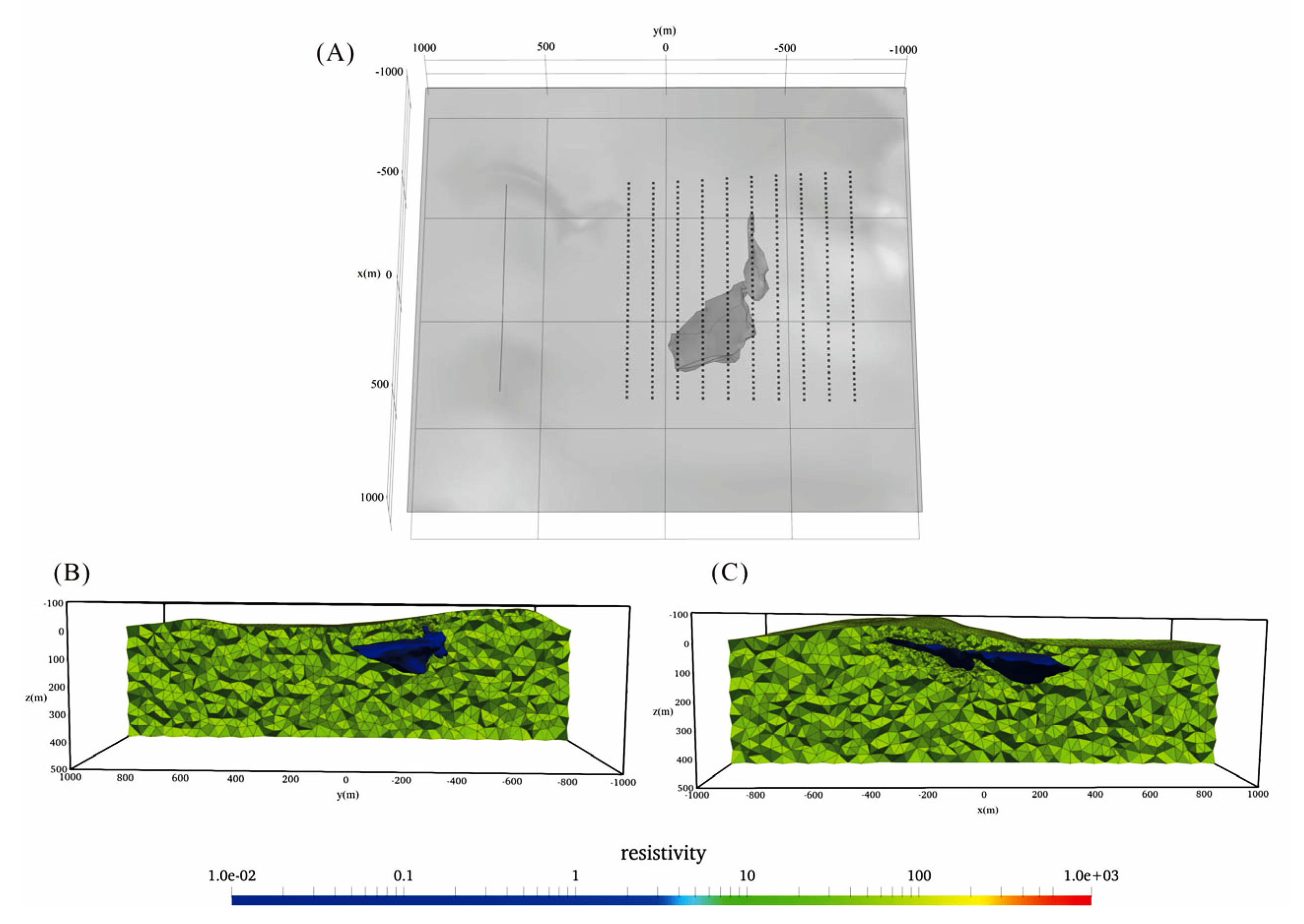
We presented a realistic model (Figure 10) as the second example. This model is an Ovoid massive sulfide deposit located at Voisey’s Bay, Labrador, Canada. The ore body is flat-lying and composed of 70 % massive sulfide. It is located under approximately 20 m of overburden [38,39,40,41] and the resistivity of the body and background is 0.01 and 100 Ω∙m, respectively. For this inversion test, we designed 10 survey lines between −750 to 150 m in the y direction with a line spacing of 100 m. There were 41 survey points on each line between −500 m and 500 m in the x direction with the interval of 25 m, and the flight altitude was 30 m. The transmitting source was 1 km long aligned in the x-axis direction, and the offset to the nearest survey point was 500 m. Figure 10A shows the source and the receivers locations with the ore body in the xy plane. Figure 10B,C show the ore body and the model discretization in the two clips from the forward model at x = −200 m and y = 0 m, respectively. The forward model was discretized into 814573 tetrahedral elements, and the inverse model was discretized into 537721 elements. All the synthetic data was contaminated by 3% Gaussian noise.

Figure 10.
The Ovoid massive sulfide ore body model. (A) shows the locations of source and survey points with the ore body (B,C) show the model discretization from two clips at x = −200 m and y = 0 m, respectively. Note that the background resistivity is also clipped to show the whole ore model.
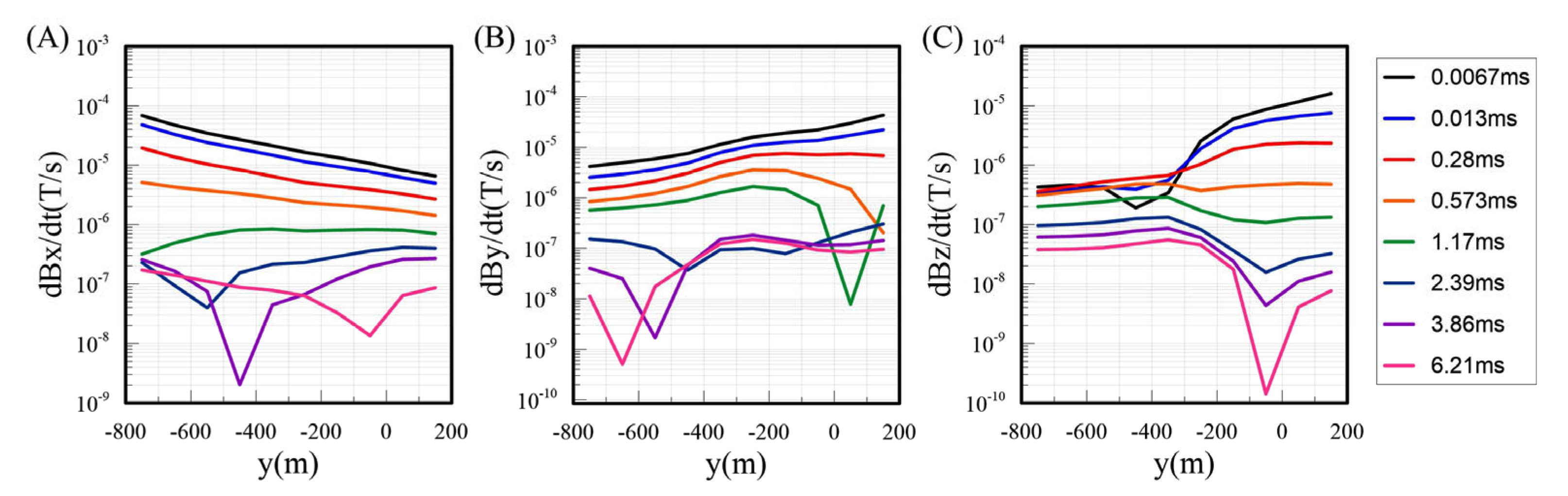
Figure 11 shows the EM responses of the sulfide deposit model at x = 50 m. Since the model was mainly horizontal, the dBz/dt component had the largest anomaly response in the early time channels (Figure 11C). However, we noticed that dBy/dt also had an obvious anomaly response that could provide information additional to the dBz/dt in the inversion.
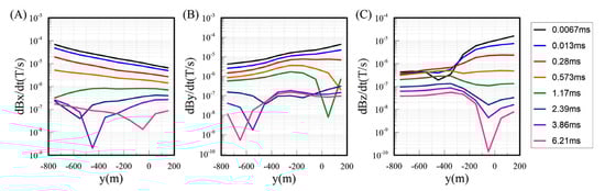
Figure 11.
Multi-component responses for the sulfide ore body model at x = 50 m. (A–C) are the X component, Y component and Z component, respectively.
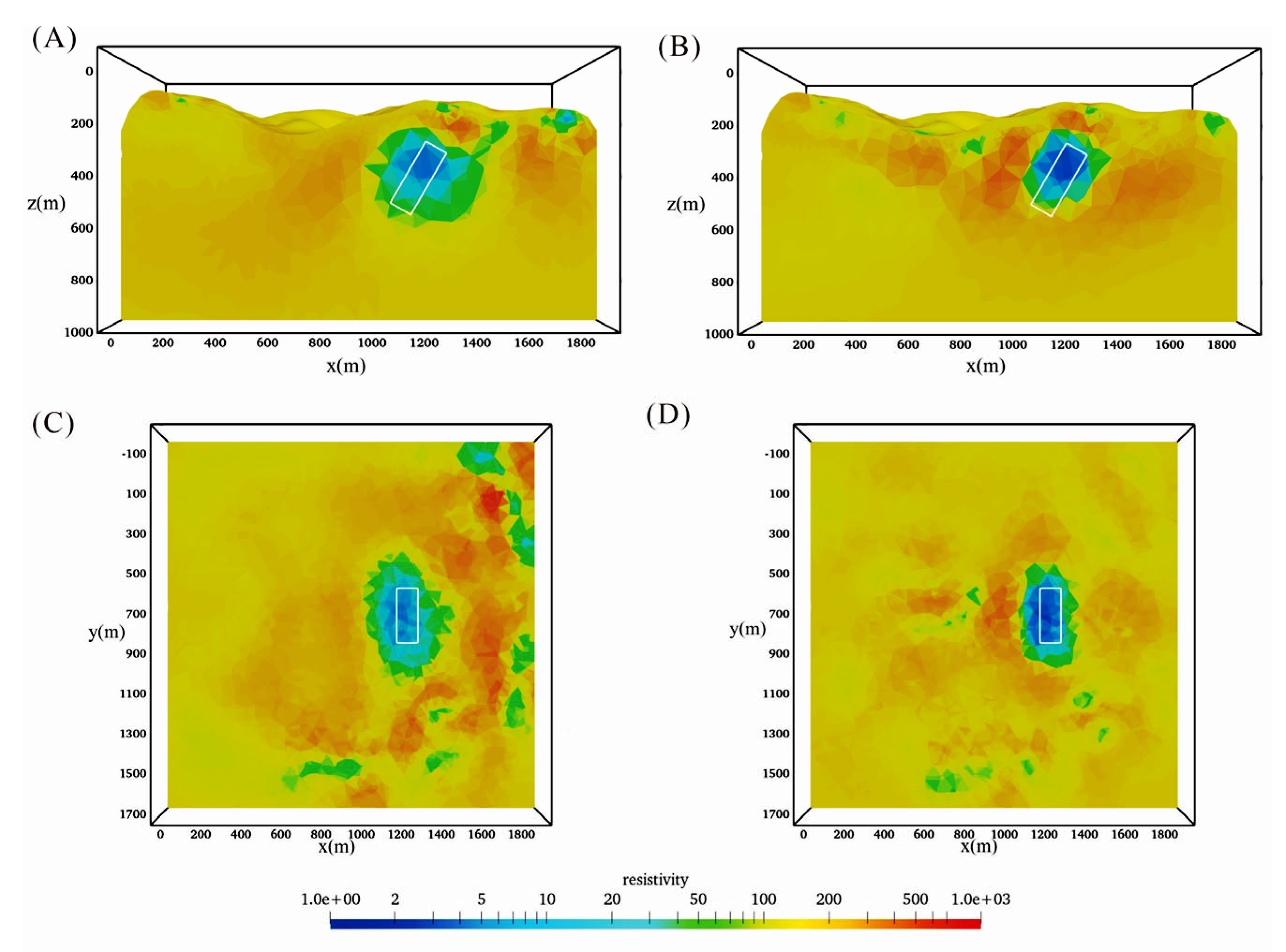
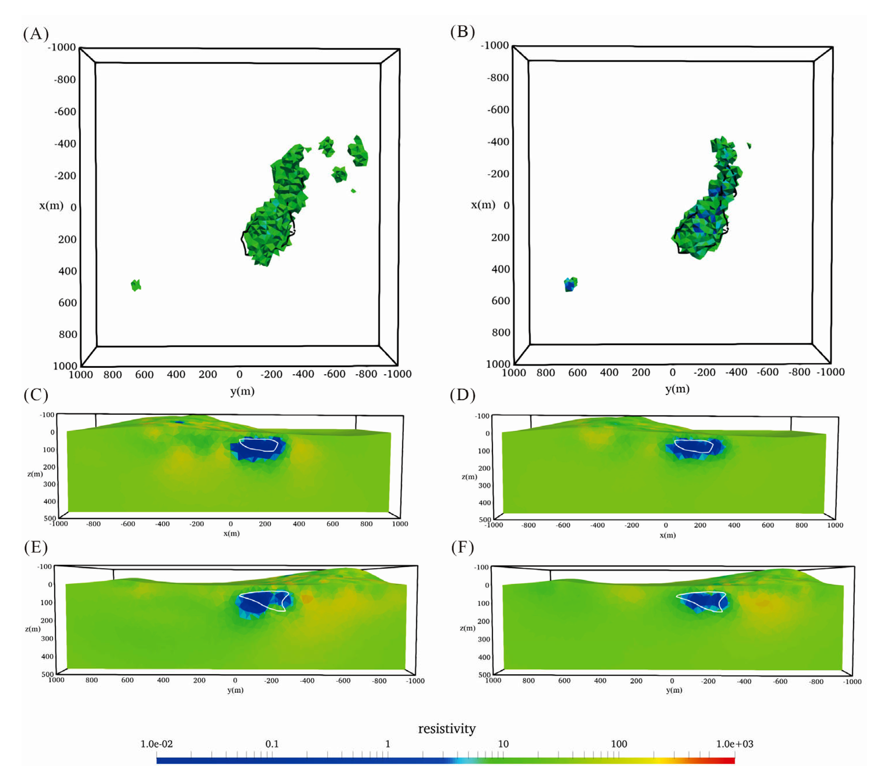
Figure 12 shows the results of the single- and multi-component inversion for the sulfide ore body model. We can see that the results of the multi-component inversion method effectively reduced the false anomalies in the inversion, and depicted the anomaly boundary more finely. This test demonstrates again that the multi-component data has obvious advantages on the improvement of resolution.
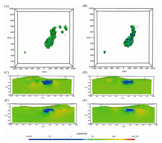
Figure 12.
Inversion results for the sulfide ore body model. (A,C,E) are the z component inversion result at z = 50 m, y = −150 m and x = 100 m (B,D,F) are the multi-component result at the same locations.
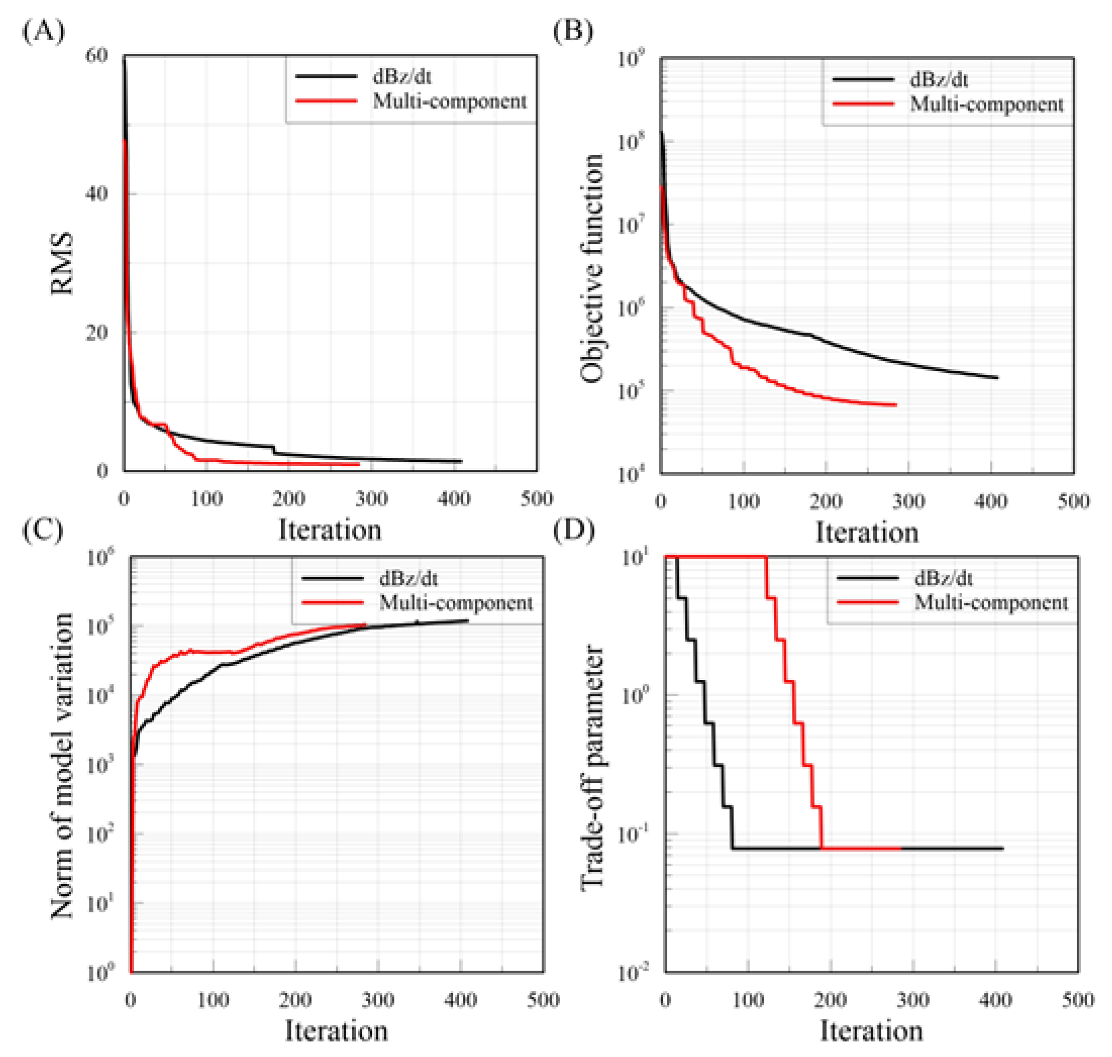
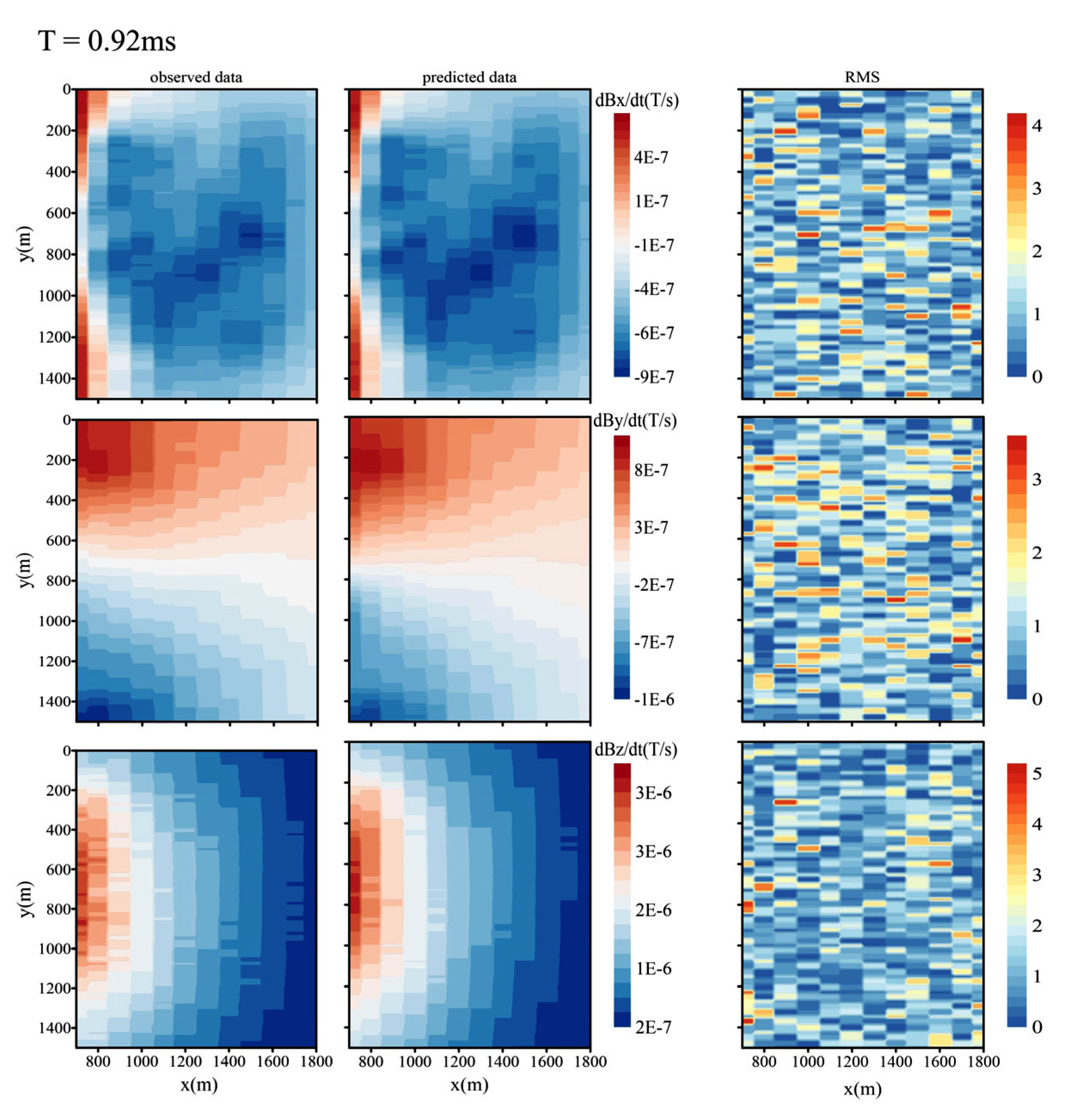
Figure 13 shows the parameters versus the iterations during the inversion progress. We can draw the same conclusion that for both inversions, the RMS, the objective function and the norm of model variation were all changing smoothly during the iteration and converged at the end of inversion, indicating the stability of the inversion algorithm. Meanwhile, compared with the single component algorithm, the multi-component inversions could converge faster because it contained more useful information from dBx/dt and dBy/dt components. Figure 14 shows the comparison between the noise-added synthetic data and the predicted data for the multi-component inversion at t = 0.92 ms. The distribution of each component of the predicted data agreed well with the observed ones, and the RMS at each survey point was distributed in the range of [0, 5] for this time channel, showing that most of the data have been fitted.
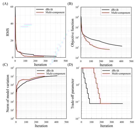
Figure 13.
Inversion parameter versus iterations for the sulfide ore body model. (A) is the RMS (B) is the objective function (C) is the norm of model variation and (D) is the trade-off parameter.
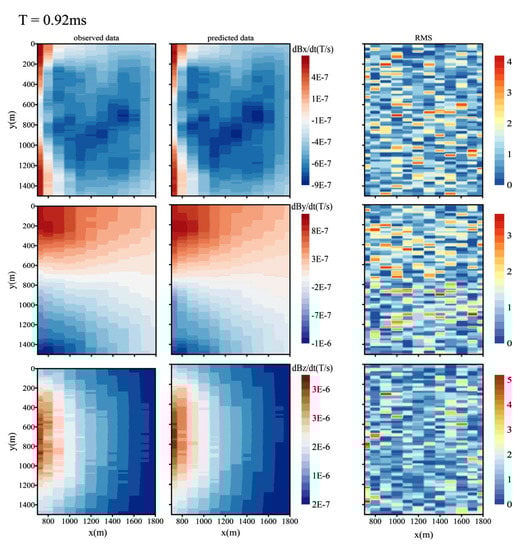
Figure 14.
Data fitting of multi-component inversion for the sulfide ore body model.
4. Conclusions
In this paper, we proposed a 3D forward and inverse algorithm for a multi-component SATEM and successfully tested it on synthetic mineral exploration models with complex terrain. The forward modeling based on the vector FE method for unstructured grids could accurately simulate arbitrary complex terrain and geological structures. After verifying the accuracy of the forward algorithm, we analyzed the detectability of the multi-component SATEM using plate models. We found that the horizontal components were more sensitive to the vertical boundaries of the anomalous body than the vertical component alone. Since there is no available SATEM field data at present, we carried out synthetic data inversion for several typical mineral models. The synthetic data for inversion was obtained by adding 3 % Gaussian noise to the forward modelled data. For all inversion examples, the initial starting model was a uniform half-space model with a resistivity of 100 Ω∙m which was chosen by trial-and-error for fast convergence. The trade-off parameter and its decay in each iteration needed to be selected appropriately by assessing various values. We observed that the inversion converges well and quickly when appropriate inversion parameters are used. The numerical experiments on two mineral exploration models showed that the inversion of the noise-added synthetic data from significant terrain recovers the anomalous bodies well. Therefore, our inversion algorithm can be used for field data interpretation. Comparing the results of multi-component inversions with those with a single component, we confirmed that the multi-component data inversion has obvious advantages to provide a more accurate and real model. The multi-component method proposed in this paper has the potential for detecting fine structures for mineral explorations in complex terrain areas. The measurement of all the components of the magnetic field decay instead of only the vertical component should be emphasized in the future development of SATEM receivers. The 3D inversion of multi-component SATEM field data will be our next target once such data are available.
Author Contributions
Z.K. implemented the algorithms, performed the analyses and wrote the manuscript. Y.L. and Y.S. came up with the idea of the method, supervised the study and review the manuscript. L.W., B.Z., X.R., Z.R. and X.M. helped in processing the data, discussing the results and drew the figures. All authors have read and agreed to the published version of the manuscript.
Funding
This paper is financially supported by the Key National Research Project of China (2021YFB3202104), the National Natural Science Foundation of China (42074120, 42274093, 42174167), Key Laboratory of Geophysical Exploration Equipment, Ministry of Education (Jilin University), China National Postdoctoral Program for Innovative Talents (BX20220130), and Guangxi Science and Technology Plan Project (2021AB30008).
Data Availability Statement
Data associated with this research are available and can be obtained by contacting the corresponding author.
Acknowledgments
Thanks to Farquharson for the Ovoid massive sulfide deposit model.
Conflicts of Interest
The authors declare no conflict of interest.
References
- Guo, W.; Dentith, M.; Xu, J.; Ren, F. Geophysical exploration for gold in Gansu Province, China. Explor. Geophys. 1999, 30, 76–82. [Google Scholar] [CrossRef]
- Cox, L.H.; Wilson, G.A.; Zhdanov, M.S. 3D inversion of airborne electromagnetic data using a moving footprint. Explor. Geophys. 2010, 41, 250–259. [Google Scholar] [CrossRef]
- Kotowski, P.O.; Becken, M.; Thiede, A.; Schmidt, V.; Schmalzl, J.; Ueding, S.; Klingen, S. Evaluation of a Semi-Airborne Electromagnetic Survey Based on a Multicopter Aircraft System. Geosciences 2022, 12, 26. [Google Scholar] [CrossRef]
- Steuer, A.; Smirnova, M.; Becken, M.; Schiffler, M.; Günther, T.; Rochlitz, R.; Yogeshwar, P.; Mörbe, W.; Siemon, B.; Costabel, S.; et al. Comparison of novel semi-airborne electromagnetic data with multi-scale geophysical, petrophysical and geological data from Schleiz, Germany. J. Appl. Geophys. 2020, 182, 104172. [Google Scholar] [CrossRef]
- Becken, M.; Nittinger, C.G.; Smirnova, M.; Steuer, A.; Martin, T.; Petersen, H.; Meyer, U.; Mörbe, W.; Yogeshwar, P.; Tezkan, B.; et al. DESMEX: A novel system development for semi-airborne electromagnetic exploration. Geophysics 2020, 85, E253–E267. [Google Scholar] [CrossRef]
- Smirnova, M.; Becken, M.; Nittinger, C.; Yogeshwar, P.; Mörbe, W.; Rochlitz, R.; Steuer, A.; Costabel, S.; Smirnov, M.; on behalf of the DESMEX Working Group. A novel semi-airborne frequency-domain CSEM system: Three-dimensional inversion of semi-airborne data from the flight experiment over an ancient mining area near Schleiz, Germany. Geophysics 2019, 84, E281–E292. [Google Scholar] [CrossRef]
- Smirnova, M.; Juhojuntti, N.; Becken, M.; Smirnov, M.; Yogeshwar, P.; Steuer, A.; Rochlitz, R.; Schiffler, M.; on behalf of the DESMEX Working Group. Combined 3D Inversion of Ground and Airborne Electromagnetic Data over Iron Ore in Kiruna. Ext. Abstr. In Proceedings of the 25th European Meeting of Environmental and Engineering Geophysics, The Hague, The Netherlands, 8–12 September 2019; p. 5. [Google Scholar] [CrossRef]
- Nabighian, M.N. Electromagnetic Methods in Applied Geophysics: Voume 1, Theory; Society of Exploration Geophysicists: Tulsa, OK, USA, 1988. [Google Scholar] [CrossRef]
- Elliott, P. New airborne electromagnetic method provides fast deep-target data turnaround. Lead. Edge 1996, 15, 309–310. [Google Scholar] [CrossRef]
- Elliott, P. Method and Apparatus of Interrogating a Volume of Material Beneath the Ground Including a Vehicle with a Detector Being Synchronized with a Generator in a Ground Loop. U. S. Patent 5610523, 3 November 1997. [Google Scholar]
- Elliott, P. The principles and practice of FLAIRTEM. Explor. Geophys. 1998, 29, 58–60. [Google Scholar] [CrossRef]
- Smith, R.S.; Annan, A.P.; McGowan, P.D. A comparison of data from airborne, semi- airborne, and ground electromagnetic systems. Geophysics 2001, 66, 1379–1385. [Google Scholar] [CrossRef]
- Yang, D.; Oldenburg, D.W. 3D inversion of total magnetic intensity data for time-domain EM at the Lalor massive sulphide deposit. Explor. Geophys. 2016, 48, 110–123. [Google Scholar] [CrossRef]
- Mogi, T.; Tanaka, Y.; Kusunoki, K.; Morikawa, T.; Jomori, N. Development of grounded electrical source airborne transient EM (GREATEM). Explor. Geophys. 1998, 29, 61–64. [Google Scholar] [CrossRef]
- Ito, H.; Mogi, T.; Jomori, A.; Yuuki, Y.; Kiho, K.; Kaieda, H.; Suzuki, K.; Tsukuda, K.; Abdallah, S. Further investigations of underground resistivity structures in coastal areas using grounded-source airborne electromagnetics. Earth Planets Space 2011, 63, e9–e12. [Google Scholar] [CrossRef]
- Ito, H.; Kaieda, H.; Mogi, T.; Jomori, A.; Yuuki, Y. Grounded electrical-source airborne transient electromagnetics (GREATEM) survey of Aso Volcano, Japan. Explor. Geophys. 2014, 45, 43–48. [Google Scholar] [CrossRef]
- Ji, Y.J.; Wu, Q.; Wang, Y.; Lin, J.; Li, D.S.; Du, S.Y.; Yu, S.B.; Guan, S.S. Noise reduction of grounded electrical source airborne transient electromagnetic data using an exponential fitting-adaptive Kalman filter. Explor. Geophys. 2018, 49, 243–252. [Google Scholar] [CrossRef]
- Huang, H.; Rudd, J. Conductivity-depth imaging of helicopter-borne TEM data based on a pseudolayer half-space model. Geophysics 2008, 73, F115–F120. [Google Scholar] [CrossRef]
- Minsley, B. A trans-dimensional Bayesian Markov chain Monte Carlo algorithm for model assessment using frequency-domain electromagnetic data. Geophys. J. Int. 2011, 187, 252–272. [Google Scholar] [CrossRef]
- Dilz, R.J.; van Kraaij, M.G.M.M.; van Beurden, M.C. A 3D spatial spectral integral equation method for electromagnetic scattering from finite objects in a layered medium. Opt. Quantum Electron. 2018, 50, 206. [Google Scholar] [CrossRef]
- Takekawa, J.; Mikada, H. A mesh-free finite-difference method for elastic wave propagation in the frequency-domain. Comput. Geosci. 2018, 118, 65–78. [Google Scholar] [CrossRef]
- Mensah, V.; Hidalgo, A.; Ferro, R.M. Numerical modelling of the propagation of diffusive-viscous waves in a fluid-saturated reservoir using finite volume method. Geophys. J. Int. 2019, 218, 33–44. [Google Scholar] [CrossRef]
- Mulligan, R.P.; Franci, A.; Celigueta, M.A.; Take, W.A. Simulations of Landslide Wave Generation and Propagation Using the Particle Finite Element Method. J. Geophys. Res. Ocean. 2020, 125, e2019JC015873. [Google Scholar] [CrossRef]
- Schwarzbach, C.; Börner, R.U.; Spitzer, K. Three-dimensional adaptive higher order finite element simulation for geo-electromagnetics—A marine CSEM example. Geophys. J. Int. 2011, 187, 63–74. [Google Scholar] [CrossRef]
- Commer, M.; Newman, G.A. New advances in three-dimensional controlled-source electromagnetic inversion. Geophys. J. Int. 2008, 172, 513–535. [Google Scholar] [CrossRef]
- Zhang, B.; Engebretsen, K.W.; Fiandaca, G.; Cai, H.; Auken, E. 3D inversion of time-domain electromagnetic data using finite elements and a triple mesh formulation. Geophysics 2021, 86, E257–E267. [Google Scholar] [CrossRef]
- Ma, H.; Tan, H.; Guo, Y. Three-Dimensional Induced Polarization Parallel Inversion Using Nonlinear Conjugate Gradients Method. Math. Probl. Eng. 2015, 2015 Pt 8, 464793.1–464793.12. [Google Scholar] [CrossRef]
- Liu, Y.H.; Yin, C.C.; Qiu, C.K.; Hui, Z.J.; Zhang, B.; Ren, X.Y.; Weng, A.H. 3-D inversion of transient EM data with topography using unstructured tetrahedral grids. Geophys. J. Int. 2019, 217, 301–318. [Google Scholar] [CrossRef]
- Oldenburg, D.W.; Haber, E.; Shekhtman, R. Three-dimensional inversion of multisource time domain electromagnetic data. Geophysics 2013, 78, E47–E57. [Google Scholar] [CrossRef]
- Rong, Z.; Liu, Y.; Yin, C.; Wang, L.; Ma, X.; Qiu, C.; Zhang, B.; Ren, X.; Su, Y.; Weng, A. Three-dimensional magnetotelluric inversion for arbitrarily anisotropic earth using unstructured tetrahedral discretization. J. Geophys. Res. Solid Earth 2022, 127, e2021JB023778. [Google Scholar] [CrossRef]
- Yin, C.C.; Hodges, G. Influence of displacement currents on the response of helicopter electromagnetic systems. Geophysics 2005, 70, G95–G100. [Google Scholar] [CrossRef]
- Nédélec, J.C. Mixed finite elements in R3. Numer. Math. 1980, 35, 315–341. [Google Scholar] [CrossRef]
- Jin, J.M. The Finite Element Method in Electromagnetics; John Wiley & Sons: Hoboken, NJ, USA, 2014. [Google Scholar]
- Haber, E. Computational Methods in Geophysical Electromagnetics. SIAM: Philadelphia, PA, USA, 2014. [Google Scholar]
- Um, E.S.; Harris, J.M.; Alumbaugh, D.L. 3D time-domain simulation of electromagnetic diffusion phenomena: A finite-element electric-field approach. Geophysics 2010, 75, F115–F126. [Google Scholar] [CrossRef]
- Amestoy, P.R.; Guermouche, A.; L’Excellent, J.Y.; Parlet, S. Hybrid scheduling for the parallel solution of linear systems. Parallel Comput. 2006, 32, 136–156. [Google Scholar] [CrossRef]
- Tikhonov, A.N.; Arsenin, V.Y. Soulutions of Ill-Posed Problems. SIAM Rev. 1977, 21, 266. [Google Scholar] [CrossRef]
- Balch, S.J. Ni-Cu Sulphide Deposits with Examples from Voisey’s Bay. In Geophysics in Mineral Exploration: Fundamentals and Case Histories; Lowe, C., Thomas, M.D., Morris, W.A., Eds.; Geological Association of Canada: St. John’s, NL, Canada, 1999. [Google Scholar]
- Jahandari, H.; Farquharson, C.G. A finite-volume solution to the geophysical electromagnetic forward problem using unstructured grids. Geophysics 2014, 79, E287–E302. [Google Scholar] [CrossRef]
- Jahandari, H.; Farquharson, C.G. Finite-volume modelling of geophysical electromagnetic data on unstructured grids using potentials. Geophys. J. Int. 2015, 202, 1859–1876. [Google Scholar] [CrossRef]
- Ansari, S.M.; Farquharson, C.G.; MacLachlan, S.P. A gauged finite-element potential formulation for accurate inductive and galvanic modelling of 3-D electromagnetic problems. Geophys. J. Int. 2017, 210, 105–129. [Google Scholar] [CrossRef]

Disclaimer/Publisher’s Note: The statements, opinions and data contained in all publications are solely those of the individual author(s) and contributor(s) and not of MDPI and/or the editor(s). MDPI and/or the editor(s) disclaim responsibility for any injury to people or property resulting from any ideas, methods, instructions or products referred to in the content. |
© 2023 by the authors. Licensee MDPI, Basel, Switzerland. This article is an open access article distributed under the terms and conditions of the Creative Commons Attribution (CC BY) license (https://creativecommons.org/licenses/by/4.0/).