Effect of Particle Shape on Parameter Calibration for a Discrete Element Model for Mining Applications

Abstract

The discrete element method (DEM) has been widely employed to model processes in different industries, such as mining, agriculture, pharmaceuticals, and food. One of the main lines of research, and in which different authors propose several approaches, is the calibration of parameters. Bulk calibration (BCA) is a common approach used that does not necessarily represent the individual behavior of each particle. On the other hand, direct measurement (DMA) is another approach employed in some cases. This work presents a comparison between calibration of DEM model parameters with non-cohesive spherical and polyhedral particles using a combination of direct measurement and bulk calibration. BCA is employed to calibrate friction parameters and DMA to characterize shape of the particles and coefficient of restitution of the contact between particles. Experimental data from Draw Down Tests are used to calibrate the friction parameters. Numerical optimization of the parameters is conducted by altering the coefficients of friction regarding the objective variables of mass flow, final mass, shear angle, and angle of repose. Quartz, granite, and coal are calibrated, obtaining good agreement with the experimental results. The influence of particle shape is tested, proving that more complex particles obtain better results for the analyzed case.

1. Introduction

The discrete element method (DEM) has progressed as an analytical tool for various bulk materials in diverse industries, such as mining, pharmaceutical, and food. In the mining industry, DEM has been widely used to model all types of machines [1], such as SAG mills [2], vibrating screens [3], cone crushers [4], gyratory crushers [5], and jaw crushers [6], in order to provide information about the design, optimization, and operation of these types of equipment. The ore, from run-of-mine, has an irregular shape and a broad particle size distribution prior to the comminution process. Because of this, it is almost impossible to model the exact shape and size of each particle. Furthermore, the calibration of contact parameters of these irregular-shaped particles cannot be accurately measured through experimental methods [7]. Therefore, a better calibration of parameters is required to improve the prediction of these numerical models [8].

In total, two general approaches are used in the calibration: direct measurement (DMA) and bulk calibration (BCA) [9]. Density calibration will be used as an example to differentiate both approaches. With direct measurement, the material density of a sample of particles would be measured individually, and a representative value (mean) would be used in the model without considering the modeled particle shape that will affect the porosity of the simulated particles. Instead, in bulk calibration, a sample is chosen, and the bulk density of the entire sample is measured. With these data and with a defined particle shape and size distribution, the material density is adjusted in the DEM model to achieve the same bulk density.

In DEM models, the parameters usually calibrated are particle shape, particle size distribution, coefficient of restitution, contact stiffness, particle density, friction coefficients (between particles and particle-boundary), and rolling resistance, among others [10], as is presented in

Table 1. List of parameters to be calibrated in a DEM simulation of non-cohesive particles.

Parameter
Particle shape	Particle size distribution
Coefficient of restitution, e	Contact stiffness
Particle density, $\rho$	Young’s Modulus, E
Coefficient of friction, $\mu$	Coefficient of rolling friction ${\mu }_r$

. For different calibration parameters, researchers have established several methods to optimize this process, such as the design of experiment, neural network method based on Latin hypercube sampling, and artificial neural network method [7]. Rackl and Hanley [11] presented a methodical calibration approach based on Latin hypercube sampling and Kriging implemented in LIGGGHTS and GNU Octave. Particle density, friction coefficients, and Young modulus were calibrated in function of repose and bulk density tests. Zhou et al. [12] established a radial basis function neural network to calibrate particle density, sliding frictions, coefficients of restitution, and Poisson’s ratio regarding the angle of repose and bulk density using the EDEM commercial software. Westbrink et al. [13] proposed a novel approach for DEM calibration with a parameter optimization based on multi-objective reinforcement learning. Richter et al. [14] showed a new modular algorithm called generalized surrogate modeling-based calibration. Using surrogate models and the Draw Down Test, the friction coefficients of a DEM model with spherical particles are calibrated. Boikov et al. [15] presented a universal calibration approach by conducting full-scale symmetrical experiments in a DEM simulation in Rocky DEM. The friction coefficient and restitution coefficients were calibrated using computer vision and an iterative calculation.

Degrassi et al. [16] performed a parameter calibration using Rocky DEM and a proprietary algorithm to optimize. The DEM model of the same test was compared with experimental data of angles of repose. The simulations were conducted using spherical particles, and the Hysteretic Linear Spring contact model. Nasato et al. [17] used artificial neural networks to calibrate static and rolling friction in function of the dynamic angle of repose and void fraction. Richter and Will [18] described a new method called metamodel-based Global Calibration. The metamodel was trained with data from several hundred simulation runs and can predict simulation responses based on a given parameter set with very high accuracy. In addition, commercial codes such as EDEM and Rocky DEM perform their calibration procedure with preconfigured simulations and post-processing scripts.

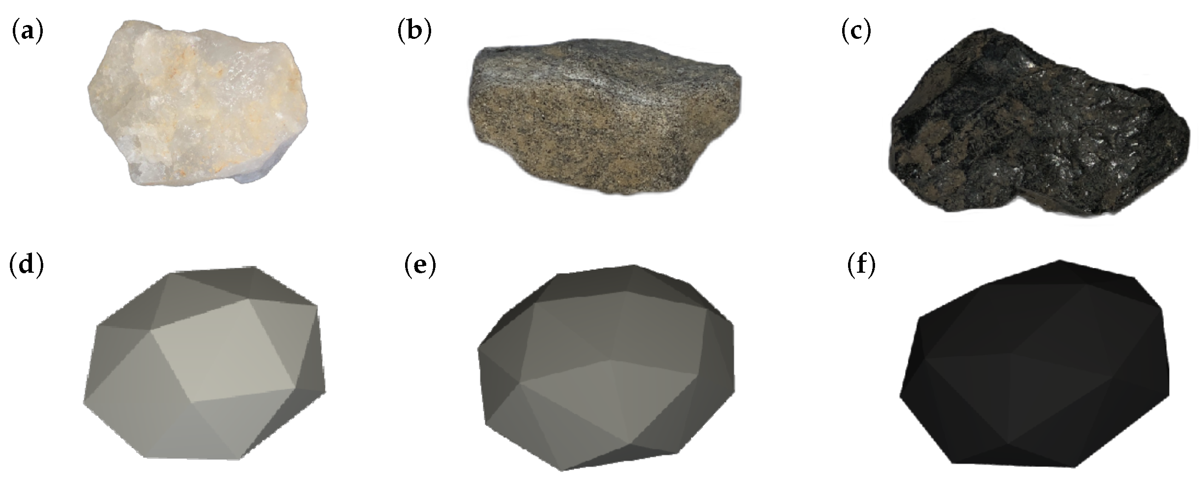
The selection of particle shape is between two main options: spherical and non-spherical particles. Spheres are used from the beginning of the formulation of DEM, and the main advantage is the simplicity and low computational cost [19]. In this approach, rolling resistance is used to numerically provide non-sphericity to the particles [20]. Moreover, despite the significant simplification in their geometric representation, spherical particles can achieve results close to the experimental ones [20,21]. An alternative to spheres is to use multi-spherical particles, which are clustered-spherical-particle that represent more complex shapes. Although the multi-sphere method represents advancement compared to the use of simple spherical bodies for approximating complex three-dimensional shapes, it is a method based on estimations that may introduce new errors itself at least on the single grain level [22]. Nevertheless, researchers state that it is necessary to simulate with non-spherical particles and can represent various particle types in granular matters [23,24,25,26]. In mining applications, bucket–-soil interaction [24], grinding mills [27], bucket filling for a mining rope shovel [26], hopper [28], cyclone [29], cone crusher [4], and gyratory crusher [5] were modeled with polyhedral particles. Mathematically, spherical particles are characterized only by their size (one parameter), and polyhedral particles can be represented by their size and four geometrical parameters. Polyhedral particles, therefore, add more parameters to the calibration.

There are several alternatives available to calibrate the coefficient of friction between particles (sliding and rolling) [30]. The most common and straightforward is measurement of the angle of repose. The disadvantage of this test is that it relates a single parameter (angle of repose) with at least two variables (friction coefficients). This means that there will then be more than one solution to the mathematical problem. Roessler et al. 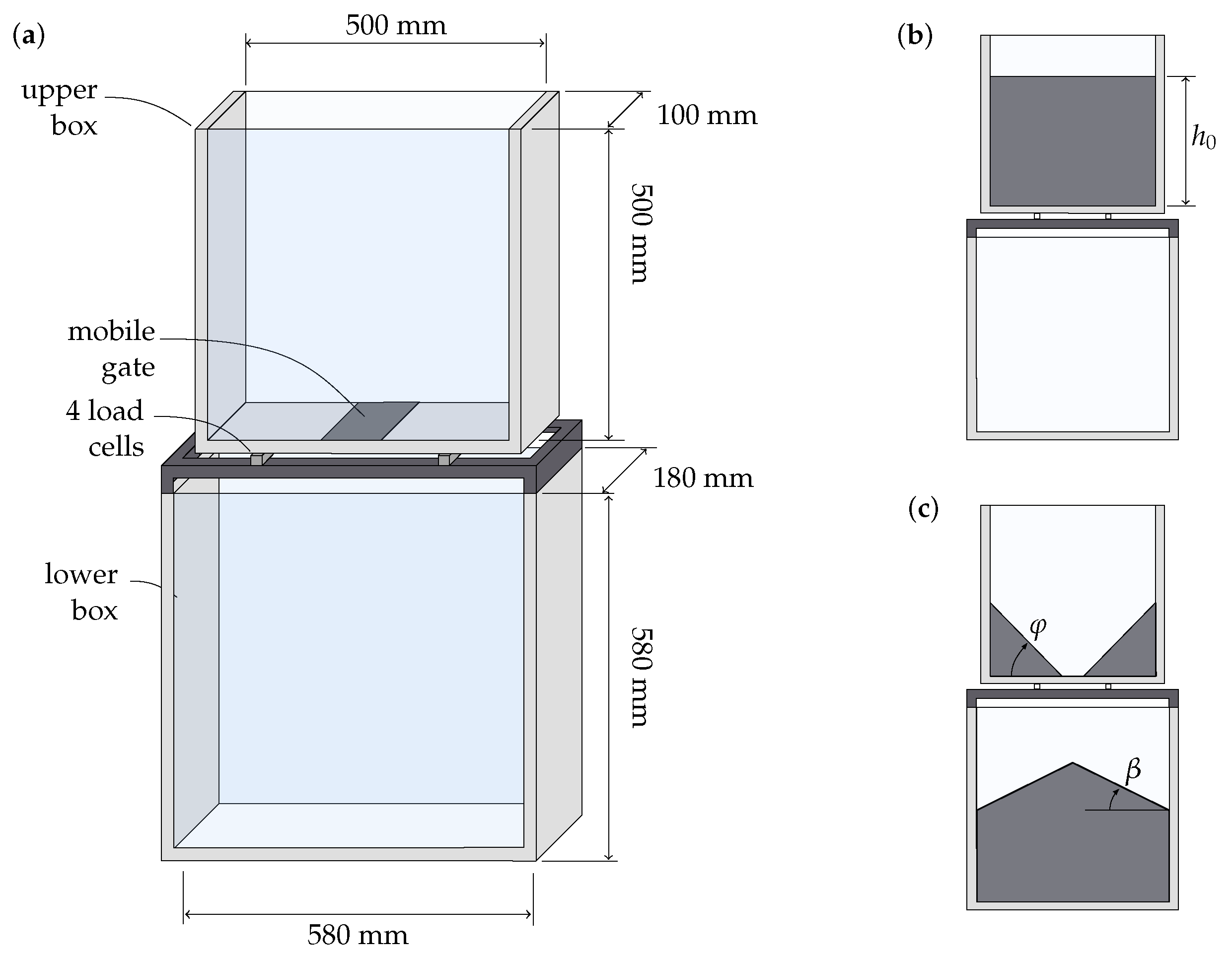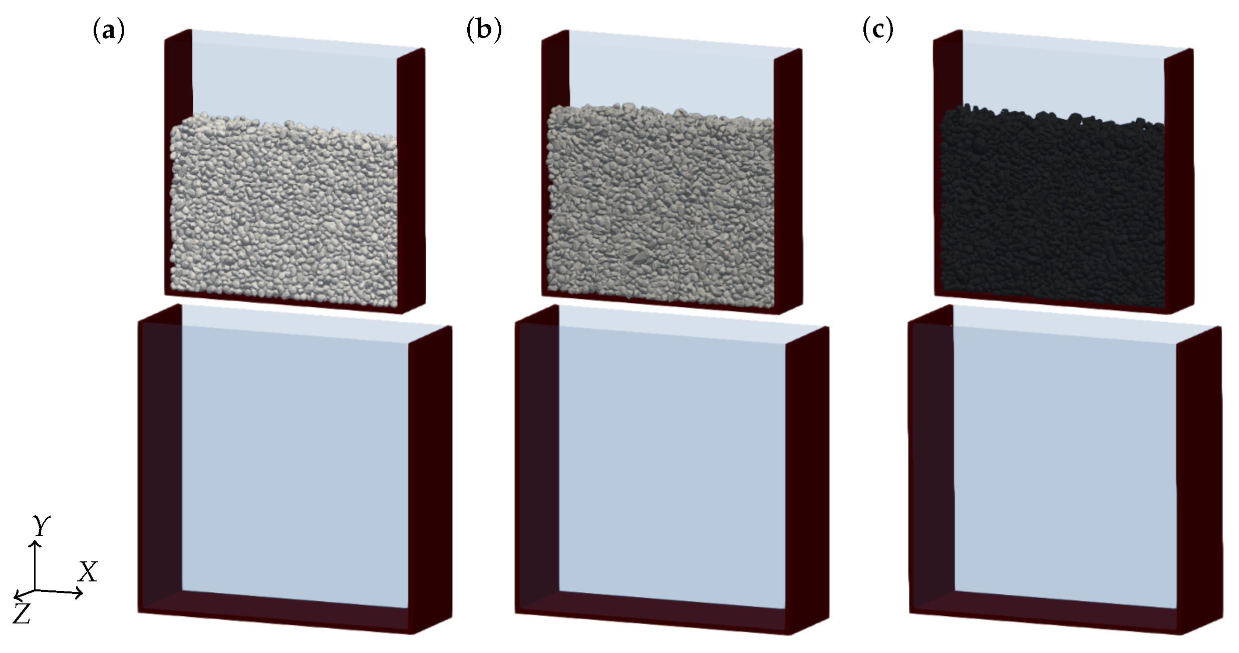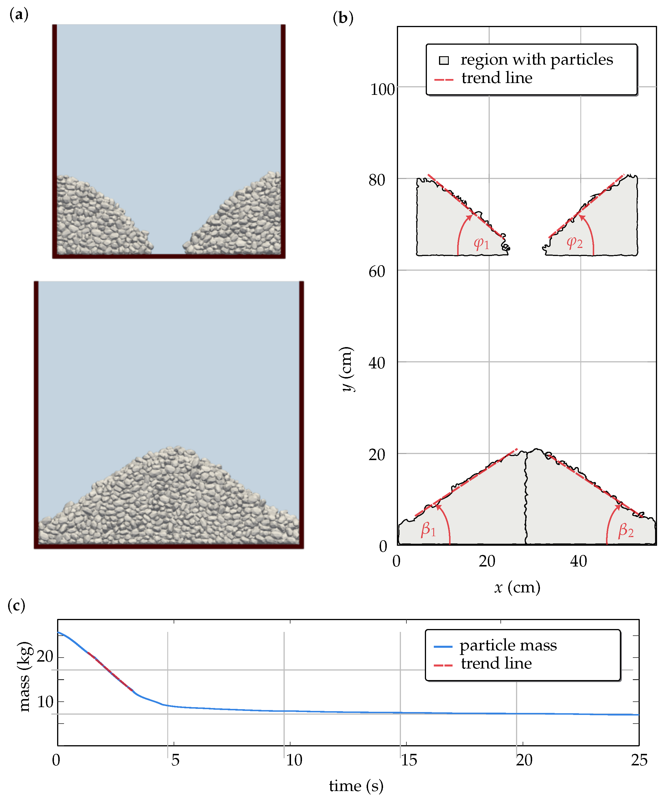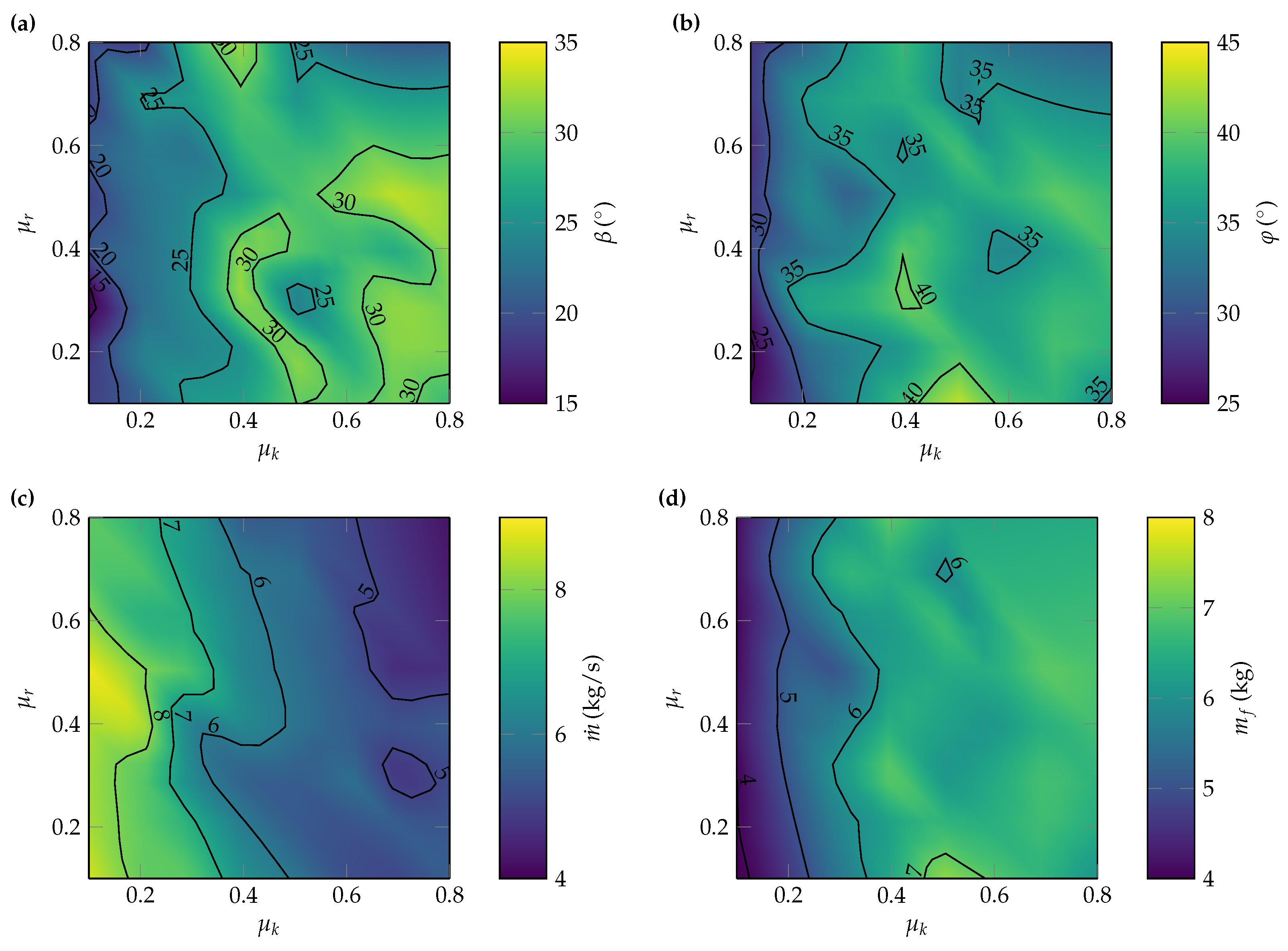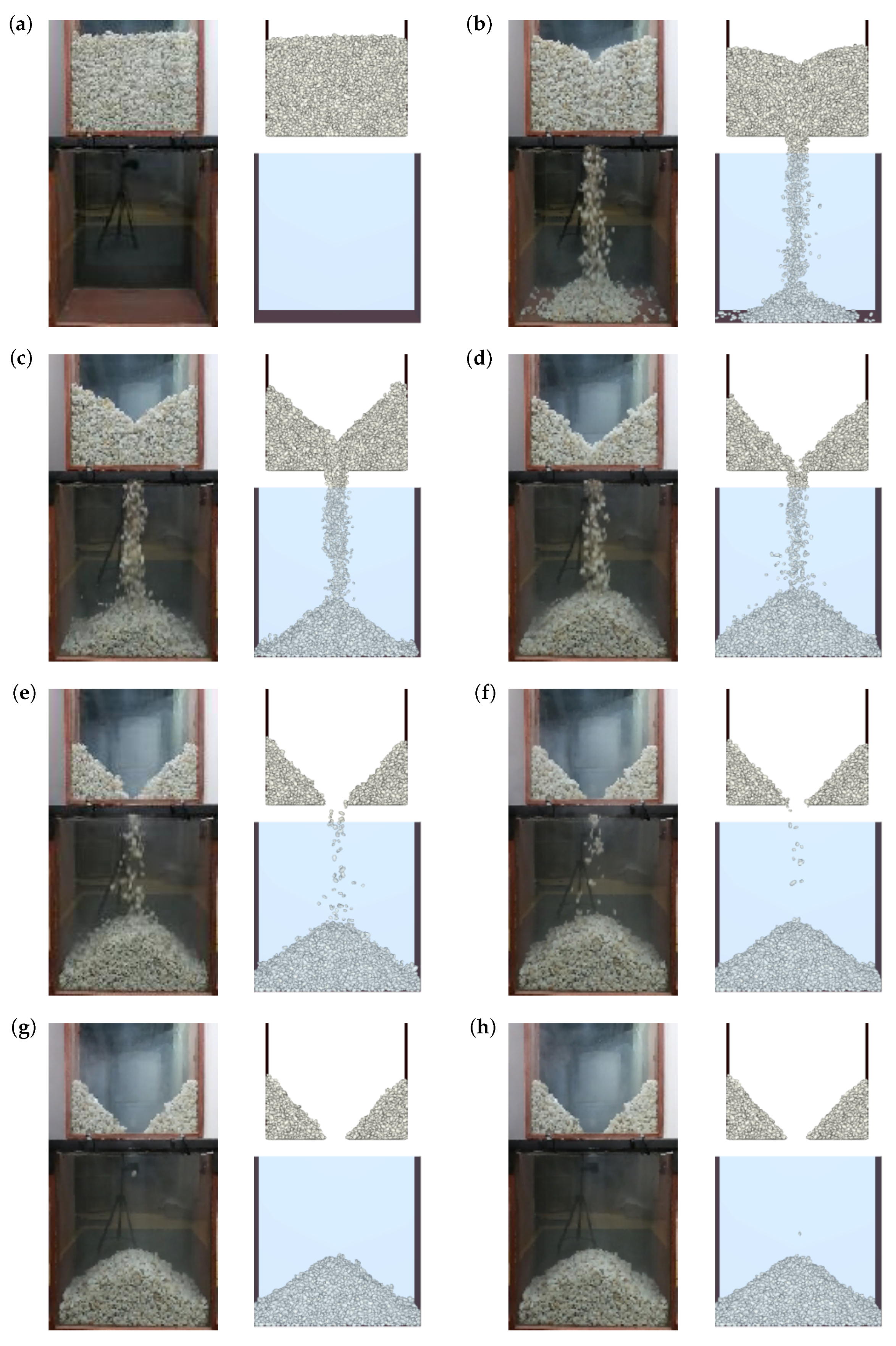[31] proposed an experimental test called Draw Down Test (DDT), which through a single experiment, allows four experimental results to be obtained: angle of repose, shear angle, mass flow rate, and final mass, which are directly contrasted with results of the DEM model. Adjusting the coefficients of friction between particles makes it possible to find a set of parameters that predicts the experimental results and avoids calibration ambiguity.

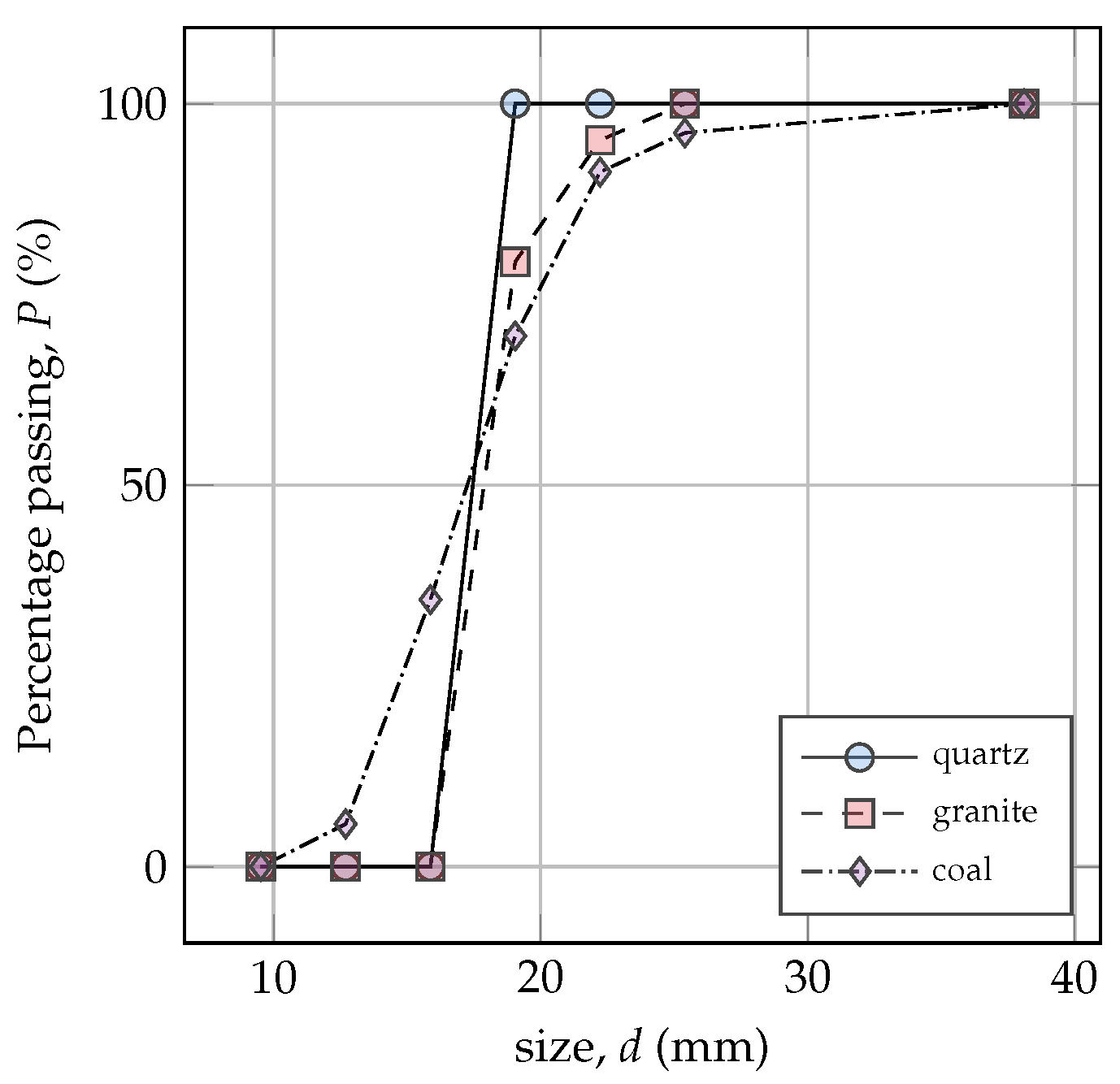
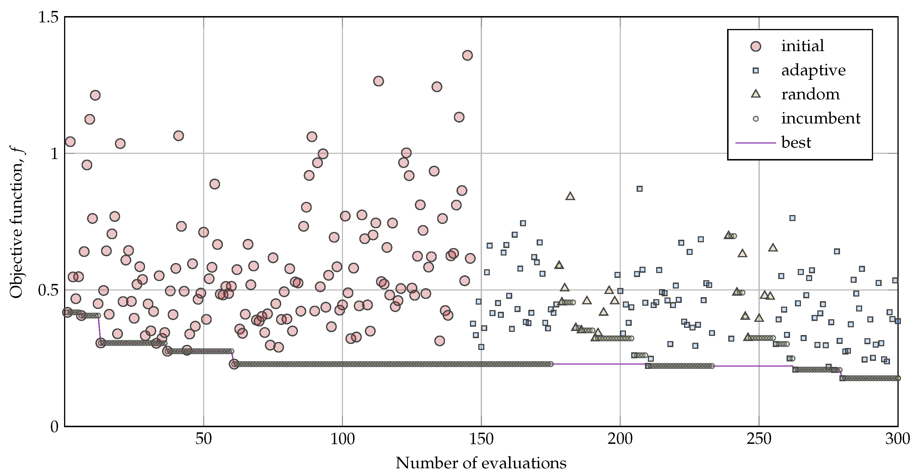
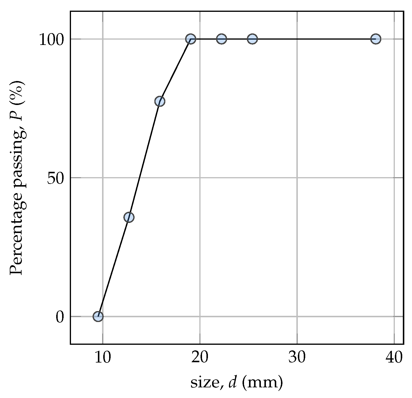
In this work, the contact parameters of three materials are calibrated for use in DEM models with non-cohesive spherical and polyhedral particles using a combination of BCA and DMA, with the aim of comparing the influence of shape on the calibration of the coefficient of friction. The DEM simulations are performed using Rocky DEM software to calibrate the friction coefficients as a function of the angle of repose, shear angle, mass flow rate, and final mass for each material with experimental data of Draw Down Tests. Experimental tests are performed to measure the particle shape directly, coefficients of restitution, and friction coefficient between particles and boundaries. The search for the combination of parameters is an optimization problem where the objective function is computationally expensive. Consequently, the number of iterations must be kept under control. In order to deal with the task, a surrogate model with radial basis functions is utilized. The influence of particle shape is studied, comparing the calibrated parameters: static coefficient of friction, dynamic coefficient of friction, and rolling friction, with spherical and polyhedral particles.

2. Materials and Methods

2.1. Materials

The ore samples used in the experiments correspond to quartz (milky quartz), gravel (granite), and coal obtained from local mines and quarries in Chile. These are cleaned, dried, and high aspect ratio particles are removed. The size ranges from 0.5 to 1 in, and all samples are properly sieved according to ASTM E-11 standard [32].

Table 2. Mass, material density, and moisture of the samples of quartz, granite and coal.

Material	Mass (kg)	Material Density (kg/m3)	Moisture (%)
Quartz	25.75	2604.1	0.5
Granite	27.75	2456.9	1.2
Coal	14.52	1324.2	1.6

presents the mass, material density [33] and moisture [34] of the samples. The particle size distribution of each sample is presented in Figure 1.

2.2. Discrete Element Method

In the discrete element method, particles and boundaries are simulated such as rigid bodies. Contact forces are typically modeled as damping-spring systems, considering their overlap distance. In this work, the normal contact force is modeled with the hysteretic linear spring model proposed by Walton and Braun [35] and the linear spring Coulomb limit for the tangential component of the force. According to the following set of equations, for the time step i, the normal contact model is:

$$F_{n,i}=\left\{\begin{array}{cc}min\left(K_{nl}·s_{n,i},F_{n,i-1}+K_{nu}·\Delta s_n\right)\hfill & ,\mathrm{if}\Delta s_n⩾0\hfill \\ max\left(F_{n,i-1}+K_{nu}·\Delta s_n,\lambda ·K_{nl}·s_{n,i}\right)\hfill & ,\mathrm{if}\Delta s_n<0\hfill \end{array}\right.$$

(1)

$$\Delta s_n=s_{n,i}-s_{n,i-1}$$

(2)

where, $F_{n,i}$ and $F_{n,i-1}$ are the normal elastic–plastic contact forces at the current time, $t_i$, at the previous time, $t_{i-1}$, respectively. $\Delta s_n$ is the change in the normal contact overlap during the current time. $s_{n,i}$ and $s_{n,i-1}$ are the normal overlap values at the current and at the previous time, respectively. $K_{nl}$ and $K_{nu}$ are the values of loading and unloading contact stiffnesses, respectively.

The tangential forces, $F_t$, are represented by the linear spring Coulomb limit model:

$$F_{t,i}=min(\left|F_t^{\prime }\right|,\mu F_{n,i})\frac{F_t^{\prime }}{\left|F_t^{\prime }\right|}$$

(3)

where $F_t^{\prime }$ is the tangential force given by (4) and $\mu$ is the coefficient of friction.

$$F_t^{\prime }=F_{t,i-1}-K_t\Delta s_t$$

(4)

with $F_{t,i-1}$ the value of the tangential force at the previous time, $\Delta s_t$ the tangential relative displacement of the particles during the time step, and $K_t$ the tangential stiffness. The stiffnesses calculation is described in detail in the software technical manual [35]. The particles are modeled as both polyhedral and spherical. Polyhedral particles are characterized by four parameters: vertical aspect ratio, horizontal aspect ratio, superquadric degree, and the number of corners.

2.3. Experimental Methodology

An experimental procedure for parameter calibration is introduced, where a direct approach is used to estimate particle shape and coefficient of restitution; meanwhile, a bulk calibration approach is used for friction coefficients.

2.3.1. Particle Shape

In total, three orthogonal dimensions of at least 100 particles per ore, between 3/4 and 1 inch in size, were measured. With these values, the vertical and horizontal aspect ratios of the samples were calculated.

In addition to the aspect ratio, polyhedral particles are defined by the number of corners and the superquadric degree. These parameters are adjusted manually, giving them the appearance of actual particles. This manual adjustment is made by comparing 3D-scanned models of an actual particle with the polyhedral particles modeled in Rocky DEM using 3D modeling software.

2.3.2. Coefficient of Restitution

Tests were performed to determine the normal coefficient of restitution between particles. The experimental setup used for the collision between particles consists of a beam, a monochrome background, a length scale, test particles, and a video camera, following the experimental setup of previous investigations [36]. The particles of irregular geometry are suspended on the beam using a thin thread and collide between them. The particle tracking is conducted by video and then programmed in MATLAB. The centroid of the particle is obtained for each video frame, and then the trajectory is obtained. With the projection of the velocities in the impact line, the coefficient of restitution e is calculated with the following expression:

$$e=-\frac{v_{B,f}-v_{A,f}}{v_{B,0}-v_{A,0}}$$

(5)

2.3.3. Draw Down Test

The test bench shown in Figure 2 was manufactured, consisting of an upper and lower box, with a mobile gate at the base of the upper box. The upper box is supported by a steel frame with four load cells of 20 kg to measure the mass of ore in the upper box as a function of time. Load cells are connected to an NI 9237 module, a bridge module that contains all signal conditioning required for power and simultaneously measures up to four bridge-based sensors. Data acquisition is performed with an NI cDAQ-9172 device connected to a laptop computer. The test is also recorded on video and photographs to complement the measurements. The experiment consists of the following steps [31]:

• Feed the upper box with 20 to 30 kg of ore bearing a defined particle size distribution.
• Level the ore bed and measure the height.
• Open the top box gate to drop the ore.
• Once the ore stops falling and is at rest, the angles of repose and shear are recorded with a digital inclinometer.
• Photographs of the final state are captured.
• The ore is removed from the top box to measure its mass.

2.4. DEM Model

The Draw Down Test is modeled in DEM using Rocky DEM 4.2.0. It has been shown that choosing only one particle shape can lead to the appearance of voids that affect the flow of the ore [4]; therefore, it is studied the influence of the particle shape in the parameter calibration. The particle shape is modeled with spheres or polyhedra, according to the three simulation cases analyzed:

• Spheres (sp): spherical particles.
• 2-polyhedra (2p): polyhedral particles with two particle shapes.
• 4-polyhedra (4p): polyhedral particles with four particle shapes.

In the first case, the particles are defined only geometrically by their size, and in the other cases, the particles are defined by their size, vertical aspect ratio, horizontal aspect ratio, number of corners, and superquadric degree. A screenshot of the simulations made for the three materials with polyhedral particles is shown in Figure 3.

The setup of the DEM simulation corresponds to two processes: feeding and emptying. The initial feeding simulation consists of filling the upper box with ore, as shown in Figure 3, and achieving the height of the ore bed obtained experimentally by adjusting the bulk density [31]. Each sub-figure presents the setup of the simulation of (a) quartz, (b) granite and (c) coal having their own particle shape, particle size distribution and material properties. Adjusted bulk and material densities are shown in

Table 3. Calibrated bulk density and friction coefficients between particles and walls. ${\mu }_{pw,1}$ corresponds to the coefficient of friction between the wall of wood and the particle, and ${\mu }_{pw,2}$ corresponds to the coefficient of friction between the wall of glass and the particle.

Material	Bulk Density (kg/m${}^3$)	${\mathit{\mu }}_{\mathit{pw},1}$	${\mathit{\mu }}_{\mathit{pw},2}$
Quartz (sp)	1527	0.709	0.424
Quartz (2p)	1450	0.709	0.424
Quartz (4p)	1462	0.709	0.424
Granite	1400	0.803	0.356
Coal	703	0.792	0.326

.

Using the first part of the simulation as a basis, the emptying simulation is commenced, where the geometry of the mobile gate is removed, and the particles descend to the lower box. The end criterion of the simulation is when the magnitude of the maximum velocity of the particles is less than 0.2 m/s, and the mass of the particles in the upper box is less than 75% of the initial mass. The simulations run until that condition is met automatically, and when finished, a post-processing script is run to obtain data files.

It is noted that for these simulations, the Young’s modulus was not calibrated, and the value $E_p=10$ MPa is adopted, which does not significantly affect the results of these simulations [37]. Concerning the shape of the particles and the coefficient of restitution between particles, the parameters directly measured are used. The e between particles and wall (the glass and wooden walls of the boxes) were not calibrated, and a reference value of 0.3 was used. The experimentally obtained friction coefficients between particles and walls are shown in Table 3, and the static friction coefficient is assumed to be equal to the dynamic friction coefficient. The geometry of the walls corresponds to the boxes and the mobile gate, with the geometry shown in Figure 2. The input particle size distribution corresponds to the same used in the test to be replicated. The time step is equal to $\Delta t={10}^{-5}$ s.

Once the DEM simulation is completed, the following data must be extracted: angle of repose $\beta$, shear angle $\phi$, mass flow rate $\dot{m}$, and final mass $m_f$ for each material. For the angles of repose and shear, the geometry of the particles is imported into MATLAB, and a line is approximated with the edge that generates the front view of the particles. The mass flow is calculated with the mass versus time curve of the upper box, as well as the remaining mass of that box. These four values correspond directly to what was measured experimentally.

2.5. Optimization

The friction coefficients (static, dynamic, and rolling) are calibrated against the angle of repose, shear angle, mass flow rate, and final mass. Therefore, there are three parameters and four objective variables. To calibrate the parameters, it is approached as an optimization problem, with $\mathit{f}$ being the vector function that evaluates the DEM model regarding the vector $\mathit{x}$ containing the friction coefficients. So, it must be resolved:

$$\underset{\mathit{x}}{min}\mathit{f}\left(\mathit{x}\right)$$

(6)

subject to

$$\left\{\begin{array}{c}{\mathit{x}}_{lb}<\mathit{x}<{\mathit{x}}_{ub}\hfill \\ c\left(\mathit{x}\right)⩽0\hfill \end{array}\right.$$

(7)

with $\mathit{x}$ vector of variables or unknowns equal to $({\mu }_{s,pp},{\mu }_{k,pp},{\mu }_r)$, $\mathit{f}$ objective vector function, ${\mathit{x}}_{lb}$ lower boundary condition vector, ${\mathit{x}}_{ub}$ upper boundary condition vector, and $c\left(\mathit{x}\right)$ is the scalar function of the inequality constraint.

Multi-objective optimization reduces to a one-objective optimization by a linear scalarization of the form:

$$\underset{\mathit{x}}{min}f\left(\mathit{x}\right)=\frac{1}{4}\underset{\mathit{x}}{min}\sum _{i=1}^4{w}_i{\left({\widehat{y}}_i\left(\mathit{x}\right)-y_i\right)}^2,\mathrm{with}\sum _{i=1}^4{w}_i=1$$

(8)

subject to the same conditions (7), and with f objective scalar function, $\mathit{w}$ is the calibration weight vector, $\widehat{\mathit{y}}\left(\mathit{x}\right)$ is the predicted value or solution vector, and $\mathit{y}$ is the vector of actual or target value. The components of these vectors are represented with the subscript i. The function $f\left(\mathit{x}\right)$ is equivalent to the weighted mean square error (WMSE). The lower and upper limits were adjusted according to previous results presented in the literature [31]. The inequality constraint ensures that the dynamic friction coefficient is greater than the static one. Calibration weights are chosen to equal 2-degree changes in angles, 0.3 kg/s in mass flow, and 0.5 kg in final mass.

These DEM simulations are known for their high computational burden, so an evaluation of the function f can take between 10 min and 1 h with spherical particles and 4 and 12 h with polyhedral particles, depending on the computational resources used (GPU or CPU) and the simulation case analyzed. For these cases, the use and optimization of a surrogate function is recommended.

It was optimized using MATLAB’s surrogateopt. This algorithm, through the evaluation of random points, the interpolation of a radial basis function, and the evaluation of a merit function that considers the substitute function and the distance between the points, allows the optimization of a function with high computational costs [38].

3. Results

The experimental and DEM simulated results of the Draw Down Test are presented. Then, the optimization and validation results of this approach are delivered.

3.1. Experimental Section

In total, six representative shapes per material are selected with the geometric measurements, and the results are displayed in the

Table 4. Shape parameters of polyhedral particles. Aspect ratios, number of corners and superquadric degree of each modeled particle. For each material sample, 6 different shapes are selected.

Particle	Horizontal Aspect Ratio	Vertical Aspect Ratio	Number of Corners	Superquadric Degree
Quartz 0	1.16	0.70	20	2.00
Quartz 1	1.26	0.77	15	2.00
Quartz 2	1.40	0.71	25	2.00
Quartz 3	1.42	0.80	20	4.00
Quartz 4	1.46	0.83	10	4.50
Quartz 5	1.61	0.77	25	2.50
Granite 0	1.15	0.62	30	2.00
Granite 1	1.22	0.61	25	2.50
Granite 2	1.27	0.70	15	5.00
Granite 3	1.39	0.73	18	3.55
Granite 4	1.42	0.61	25	2.50
Granite 5	1.56	0.72	15	2.5
Coal 0	1.19	0.67	25	2.35
Coal 1	1.26	0.70	23	3.5
Coal 2	1.31	0.66	20	5.00
Coal 3	1.49	0.76	28	3.00
Coal 4	1.59	0.76	15	2.75
Coal 5	1.68	0.69	16	5.5

. The distribution of aspect ratios is statistically analyzed to select the particles, choosing six representative percentiles: 20%, 33.3%, 40%, 60%, 66.6%, and 80%. Figure 4 shows some pictures of quartz, granite, and coal, along with a modeled particle with the adjusted parameters. The 2-polyhedra case uses particles 1 and 4, and the 4-polyhedra case uses particles 0, 2, 3, and 5.

The results of the coefficients of restitution test are presented. By analyzing each test of each material and using Equation (5), the results of the

Table 5. Experimental results of the coefficient of restitution for the three sample materials.

Material	Mean	Standard Deviation
Quartz	0.3719	0.1633
Granite	0.2996	0.1212
Coal	0.2758	0.0781

are obtained. As each test is performed at different impact velocities, different geometry, and orientation of the particles, the results can present a considerable dispersion. Considering that the contact model considers a single value of the coefficient of restitution, without depending on the relative speed between the particles or orientation on impact, the average value is acceptable [39]. In Rocky DEM, it is possible to use a velocity-dependent coefficient of restitution, but the influence of contact geometry and orientation is still strong.

Regarding the experimental results of Draw Down Test, for each material, the four results are presented in the

Table 6. Experimental results of the Draw Down Test. Angle of repose, shear angle, mass flow rate and final mass of each sample.

Material	$\mathit{\beta }\left({}^{\circ }\right)$	$\mathit{\phi }\left({}^{\circ }\right)$	$\dot{\mathit{m}}$ (kg/s)	${\mathit{m}}_{\mathit{f}}$ (kg)
Quartz	26.25	42.03	4.83	7.09
Granite	32.59	45.39	3.88	7.28
Coal	22.91	47.20	2.23	3.84

. These results are the averages of three tests, so six values of each angle and three of each mass parameter are averaged. Figure 5 presents the binaries images of the photographs of the final state of a test done with coal. From these images, two angles of repose are calculated with (c) and (d), and two shear angles with (a) and (b), which is performed by detecting the edge and then calculating its slope numerically. The mass parameters are calculated from the measured mass signal over time, the mass flow rate through the slope, and the final mass with the last values of the graph. The final mass is also verified by measuring the mass remaining in the top box on a scale.

3.2. DEM

As an example, a DEM simulation of DDT with quartz is detailed. There are feed 25.75 kg of quartz simulated with four polyhedral particles, in size range of 1/2 and 3/4 in, and the average results of this experimental test are presented in Table 6. In these simulations, the height of the ore was 330 mm, achieving an bulk density of 1462 kg/m³.

Figure 6 shows an example of a simulation and analysis done with ${\mu }_s$ = 0.7, ${\mu }_k$ = 0.7 and ${\mu }_r$ = 0.5. Figure 6a shows a screenshot of the end of the DEM simulation, showing the distribution of the particles in both boxes. By exporting particle information such as shape, size, position, and orientation, it is possible to fully reproduce the geometry of each polyhedral particle in MATLAB and obtain the edge of the projected surface in the front view, as shown in Figure 6b. With the edge, a linear trend line can calculate the angles of interest. Two angles of shear (${\phi }_1$ and ${\phi }_2$) and of repose (${\beta }_1$ and ${\beta }_2$) are obtained; the value to use is the average of both results. The mass of the particles in the top box, shown in Figure 6c, is analyzed. The mean mass flow rate is calculated with the slope and the final mass taking the last value on the graph.

When calculating the simulated results, it is obtained: $\beta ={33.36}^{\circ }$, $\phi ={40.26}^{\circ }$, $\dot{m}=4.59$ kg/s and $m_f=7.02$ kg, and the error is $\mathrm{WSME}=0.4967$. These results differ significantly from the experimental ones. Hence, it is necessary to search for the optimal values of the friction coefficients.

3.3. Optimization

To begin the calibration of parameters and obtain initial values, the condition is analyzed in which the coefficient of sliding friction is equal to the static one, ${\mu }_s={\mu }_k$, as presented in the literature [31]. ${\mu }_k$ and ${\mu }_r$ are varied between 0.1 and 0.8, and the results of Figure 7 are presented. Each graph represents the behavior of the variable regarding the sliding coefficient and the rolling coefficient, describing a surface. These response surfaces are different from those presented in the literature [30,31] because they are calibrated for polyhedral particles instead of spherical particles. These graphs help find the ranges of values that yield better results. Consequently, the best results are the pair 0.8 and 0.1, with $\beta ={28.31}^{\circ }$, $\phi ={43.45}^{\circ }$, $\dot{m}=5.21$ kg/s and $m_f=7.57$ kg, with an error of $\mathrm{WSME}=0.2323$. These results are closer to the experimental ones than the initial ones, but they can be improved by adding the calibration of the static coefficient of friction.

With the calibration of ${\mu }_k$ and ${\mu }_r$ as initial values, the static friction coefficient is calibrated. The upper and lower limits of the optimization are extended according to the optimal value found previously. The literature does not calibrate this parameter since the contact model used only considers the coefficient of sliding friction [18,31]. Boikov et al. [15] performed the calibration of this parameter without optimization.

Optimization is restricted between 400 and 600 iterations, with three significant digits in the friction coefficients and a function tolerance of 0.03. Figure 8 presents a graph of the objective function f regarding the number of evaluations of the optimization performed for quartz with 4-polyhedral particles, showing how the optimization progresses. It is observed that the algorithm can find a minimum regarding the initial samples. Only the calibration of quartz with 4-polyhedral particles is conducted with 150 initial values, in the other cases, just 50 initial values are used. The

Table 7. Results of optimization of friction parameters through Draw Draw Test DEM simulations. The calibrated parameters of each material and particle shape are presented.

Material	${\mathit{\mu }}_{\mathit{s},\mathit{pp}}$	${\mathit{\mu }}_{\mathit{k},\mathit{pp}}$	${\mathit{\mu }}_{\mathit{r}}$	$\mathit{\beta }\left({}^{\circ }\right)$	$\mathit{\phi }\left({}^{\circ }\right)$	$\dot{\mathit{m}}$ (kg/s)	${\mathit{m}}_{\mathit{f}}$ (kg)	Iterations	WMSE
Quartz (sp)	0.938	0.919	0.231	27.98	44.66	5.30	7.50	600	0.0911
Quartz (2p)	1.125	0.925	0.100	30.04	40.18	4.97	7.13	400	0.0749
Quartz (4p)	1.000	0.880	0.100	28.39	43.01	4.97	7.11	400	0.0258
Granite (sp)	0.950	0.950	0.400	33.10	47.63	4.15	8.61	600	0.1486
Granite (4p)	0.950	0.895	0.304	33.51	45.5	4.05	7.92	400	0.0365
Coal (sp)	1.128	1.017	0.273	25.84	45.37	2.66	4.25	600	0.0916
Coal (4p)	1.000	0.800	0.200	26.49	44.23	2.26	3.88	400	0.0866

shows the results of the optimizations for the three materials, the number of evaluations performed, and the WMSE.

Comparing the results obtained for quartz with different particle shapes (sp, 2p, and 4p), it is noted that due to presenting the lowest WMSE value, the case with four polyhedral particles performs best. In fact, when the particle shape is more complex, the improvement in the calibration is significant, with errors occuring less frequently. For granite and coal, when comparing the solutions of spherical and 4-polyhedral particles, a better solution is also obtained in the 4p case. In all these optimizations, a better solution is obtained with the same or less number of evaluations. The calibrated friction coefficients between the cases for each material are close, with differences of 10% at most, and for rolling friction, the maximum difference is 0.131. This means that when the particle shape is changed in a DEM simulation, using parameters calibrated with another shape could deliver good results and be improved by optimization with few iterations around the initial value. Since there is less computation time with spherical particles, these values can be used as initial values of the calibration parameters of polyhedral particles. Regarding differences in the calibrated coefficient of friction, a clear trend concerning different shapes cannot be seen, and a complete analysis is needed to relate particle shape parameters and friction coefficients. The principal difference is that spherical particles need more rolling friction to achieve the expected results. However, the mathematical relation between rolling friction parameter and non-sphericity of the particles remains unclear [40].

3.4. Validation

Another Draw Down Test was utilized to validate the proposed approach, where a quartz sample weighing 26.95 kg with the particle size distribution presented in Figure 9 is used. A DEM simulation of this test with the calibrated parameters of quartz is performed, and the results of interest are compared.

Figure 10 shows a corresponding graphical comparison of this test and its simulation in DEM. On the left is a photograph of the experimental test, and on the right is an image of the DEM simulation, for different times, from $t=0$ s to $t=7$ s. There is a good agreement between the simulated and the experimental by simply comparing the images.

The

Table 8. Validation of the calibration of friction coefficients.

Variable	$\mathit{\beta }\left({}^{\circ }\right)$	$\mathit{\phi }\left({}^{\circ }\right)$	$\dot{\mathit{m}}$ (kg/s)	${\mathit{m}}_{\mathit{f}}$ (kg)
Experimental	29.43	43.41	5.08	6.60
Simulated	28.75	34.54	6.35	6.72

presents the experimental and simulated results this test. The relative errors of the angle of repose and final mass are less than 5%, while the errors of the shear angle and mass flow are between 20 and 25%, respectively. The error of the fit is quantified by and weighted mean square error of $\mathrm{WMSE}=0.6621$.

4. Conclusions

A better fit in friction coefficients, regarding the results of a Draw Down Test, can be obtained using more complex particle shapes, as tested with quartz, granite, and coal ore modeled with 4-polyhedral particles, 2-polyhedral particles, and spherical particles. The difference in WMSE in the calibration between spherical and polyhedral particles is considerable, and the calibrated coefficients of friction change between different particle shapes. As a result, all ore samples selected are completely characterized for use in a DEM model.

The combination of bulk calibration and direct measurement of material parameters in sample models presents a viable alternative to perform, and allows for improvements in the prediction of DEM models. Optimization using a surrogate function is helpful for optimization problems where the objective function is expensive, such as in the simulations presented.

Regardless of the best fit of polyhedral particles, computation time must be considered when choosing the particle shape. For instance, in the DEM simulations analyzed, calculations with spheres occurred 24-times faster than polyhedra. Considering particle shape, calibration, and computation time, recommendations include:

• Spherical particles present the best alternative in scenarios where modeling the particle shape is not required, and it is necessary to reduce simulation times while ensuring calibration is still performed thoroughly.
• Polyhedral particles are suggested when the particle shape is essential, and precision is required in calculations. Furthermore, some DEM breakage models only work with polyhedral particles, as in the case of breakage models of the software Rocky DEM. A particle replacement model with polyhedral particles can conserve mass and volume, whereas, this is not possible with spherical particles.

Overall, a method is proposed to study less expensive optimization methods for polyhedral particles. The simulations performed with polyhedral particles incurred high computational cost, so the use of polyhedral particles might be excluded in several applications due to the expenses associated with calibration. However, its good behavior demonstrated by the model makes it pertinent to examine less expensive calibration procedures. A viable approach is through a previous calibration of spherical particles that delivers initial values of the parameters. In addition, as each application case presents a different distribution of size and shape, it is a complex process to unify a calibration method for all possible applications.

References

1. Qiu, X. DEM Simulations in Mining and Mineral Processing. In Proceedings of the 7th International Conference on Discrete Element Methods; Li, X., Feng, Y., Mustoe, G., Eds.; Springer: Singapore, 2016; pp. 37–43. [Google Scholar]
2. Venegas, J.; Valenzuela, M.A.; Molina, C. Correlation Between Power and Lifters Forces in Grinding Mills. IEEE Trans. Ind. Appl. 2019, 55, 4417–4427. [Google Scholar]
3. Peng, L.; Jiang, H.; Chen, X.; Liu, D.; Feng, H.; Zhang, L.; Zhao, Y.; Liu, C. A review on the advanced design techniques and methods of vibrating screen for coal preparation. Powder Technol. 2019, 347, 136–147. [Google Scholar] [CrossRef]
4. André, F.P.; Tavares, L.M. Simulating a laboratory-scale cone crusher in DEM using polyhedral particles. Powder Technol. 2020, 372, 362–371. [Google Scholar] [CrossRef]
5. Moncada, M.; Toledo, P.; Betancourt, F.; Rodríguez, C.G. Torque Analysis of a Gyratory Crusher with the Discrete Element Method. Minerals 2021, 11, 878. [Google Scholar] [CrossRef]
6. Barrios, G.K.; Jiménez-Herrera, N.; Fuentes-Torres, S.N.; Tavares, L.M. DEM Simulation of Laboratory-Scale Jaw Crushing of a Gold-Bearing Ore Using a Particle Replacement Model. Minerals 2020, 10, 717. [Google Scholar] [CrossRef]
7. Wang, X.; Ma, H.; Li, B.; Li, T.; Xia, R.; Bao, Q. Review on the research of contact parameters calibration of particle system. J. Mech. Sci. Technol. 2022, 36, 1363–1378. [Google Scholar] [CrossRef]
8. Windows-Yule, C.; Neveu, A. Calibration of DEM simulations for dynamic particulate systems. Pap. Phys. 2022, 14, 140010. [Google Scholar] [CrossRef]
9. Coetzee, C.J. Review: Calibration of the discrete element method. Powder Technol. 2017, 310, 104–142. [Google Scholar] [CrossRef]
10. Katterfeld, A.; Coetzee, C.; Donohue, T.; Fottner, J.; Grima, A.; Ramirez Gomez, A.; Ilic, D.; Kačianauskas, R.; Necas, J.; Schott, D.; et al. Calibration of DEM Parameters for Cohesionless Bulk Materials under Rapid Flow Conditions and Low Consolidation. White Paper 2019. [Google Scholar] [CrossRef]
11. Rackl, M.; Hanley, K.J. A methodical calibration procedure for discrete element models. Powder Technol. 2017, 307, 73–83. [Google Scholar] [CrossRef] [Green Version]
12. Zhou, H.; Hu, Z.; Chen, J.; Lv, X.; Xie, N. Calibration of DEM models for irregular particles based on experimental design method and bulk experiments. Powder Technol. 2018, 332, 210–223. [Google Scholar] [CrossRef]
13. Westbrink, F.; Elbel, A.; Schwung, A.; Ding, S.X. Optimization of DEM parameters using multi-objective reinforcement learning. Powder Technol. 2020, 379, 602–616. [Google Scholar] [CrossRef]
14. Richter, C.; Rößler, T.; Kunze, G.; Katterfeld, A.; Will, F. Development of a standard calibration procedure for the DEM parameters of cohesionless bulk materials—Part II: Efficient optimization-based calibration. Powder Technol. 2020, 360, 967–976. [Google Scholar] [CrossRef]
15. Boikov, A.; Savelev, R.; Payor, V.; Potapov, A. Universal Approach for DEM Parameters Calibration of Bulk Materials. Symmetry 2021, 13, 1088. [Google Scholar] [CrossRef]
16. Degrassi, G.; Parussini, L.; Boscolo, M.; Petronelli, N.; Dimastromatteo, V. Discrete element simulation of the charge in the hopper of a blast furnace, calibrating the parameters through an optimization algorithm. SN Appl. Sci. 2021, 3, 242. [Google Scholar] [CrossRef]
17. Nasato, D.S.; Albuquerque, R.Q.; Briesen, H. Predicting the behavior of granules of complex shapes using coarse-grained particles and artificial neural networks. Powder Technol. 2021. [Google Scholar] [CrossRef]
18. Richter, C.; Will, F. Introducing Metamodel-Based Global Calibration of Material-Specific Simulation Parameters for Discrete Element Method. Minerals 2021, 11, 848. [Google Scholar] [CrossRef]
19. Soltanbeigi, B.; Podlozhnyuk, A.; Kloss, C.; Pirker, S.; Ooi, J.Y.; Papanicolopulos, S.A. Influence of various DEM shape representation methods on packing and shearing of granular assemblies. Granul. Matter 2021, 23. [Google Scholar] [CrossRef]
20. Xie, C.; Ma, H.; Zhao, Y. Investigation of modeling non-spherical particles by using spherical discrete element model with rolling friction. Eng. Anal. Bound. Elem. 2019, 105, 207–220. [Google Scholar] [CrossRef]
21. Zhang, S.; Zsáki, A.M. Effect Geometric Detail on the Outcome of DEM Simulations with Polyhedral Particles. Geomech. Geoengin. 2022. [Google Scholar] [CrossRef]
22. Kruggel-Emden, H.; Rickelt, S.; Wirtz, S.; Scherer, V. A study on the validity of the multi-sphere Discrete Element Method. Powder Technol. 2008, 188, 153–165. [Google Scholar] [CrossRef]
23. Nassauer, B.; Liedke, T.; Kuna, M. Polyhedral particles for the discrete element method. Granul. Matter 2012, 15, 85–93. [Google Scholar] [CrossRef]
24. Nezami, E.G.; Hashash, Y.M.A.; Zhao, D.; Ghaboussi, J. Simulation of front end loader bucket–soil interaction using discrete element method. Int. J. Numer. Anal. Methods Geomech. 2007, 31, 1147–1162. [Google Scholar] [CrossRef]
25. Landauer, J.; Kuhn, M.; Nasato, D.S.; Foerst, P.; Briesen, H. Particle shape matters—Using 3D printed particles to investigate fundamental particle and packing properties. Powder Technol. 2019, 361, 711–718. [Google Scholar] [CrossRef]
26. Svanberg, A.; Larsson, S.; Mäki, R.; Jonsén, P. Full-scale simulation and validation of bucket filling for a mining rope shovel by using a combined rigid FE-DEM granular material model. Comput. Part. Mech. 2020, 8, 825–843. [Google Scholar] [CrossRef]
27. Govender, N.; Rajamani, R.; Wilke, D.N.; Wu, C.Y.; Khinast, J.; Glasser, B.J. Effect of particle shape in grinding mills using a GPU based DEM code. Miner. Eng. 2018, 129, 71–84. [Google Scholar] [CrossRef] [Green Version]
28. Govender, N.; Wilke, D.N.; Wu, C.Y.; Khinast, J.; Pizette, P.; Xu, W. Hopper flow of irregularly shaped particles (non-convex polyhedra): GPU-based DEM simulation and experimental validation. Chem. Eng. Sci. 2018, 188, 34–51. [Google Scholar] [CrossRef] [Green Version]
29. El-Emam, M.A.; Zhou, L.; Shi, W.; Han, C. Performance evaluation of standard cyclone separators by using CFD–DEM simulation with realistic bio-particulate matter. Powder Technol. 2021, 385, 357–374. [Google Scholar] [CrossRef]
30. Coetzee, C. Calibration of the discrete element method: Strategies for spherical and non-spherical particles. Powder Technol. 2020, 364, 851–878. [Google Scholar] [CrossRef]
31. Roessler, T.; Richter, C.; Katterfeld, A.; Will, F. Development of a standard calibration procedure for the DEM parameters of cohesionless bulk materials—Part I: Solving the problem of ambiguous parameter combinations. Powder Technol. 2019, 343, 803–812. [Google Scholar] [CrossRef]
32. ASTM E11-20; Specification for Woven Wire Test Sieve Cloth and Test Sieves. Standard, ASTM International: West Conshohocken, PA, USA, 2020.
33. ASTM D7263-21; Test Methods for Laboratory Determination of Density (Unit Weight) of Soil Specimens. Standard, ASTM International: West Conshohocken, PA, USA, 2021.
34. ASTM D2216-19; Test Methods for Laboratory Determination of Water (Moisture) Content of Soil and Rock by Mass. Standard, ASTM International: West Conshohocken, PA, USA, 2019.
35. ESSS. DEM Technical Manual 4.2; ESSS Rocky DEM, S.R.L.: Florianópolis, Brazil, 2018. [Google Scholar]
36. Hlosta, J.; Žurovec, D.; Rozbroj, J.; Ramírez-Gómez, Á.; Nečas, J.; Zegzulka, J. Experimental determination of particle–particle restitution coefficient via double pendulum method. Chem. Eng. Res. Des. 2018, 135, 222–233. [Google Scholar] [CrossRef]
37. Lommen, S.; Schott, D.; Lodewijks, G. DEM speedup: Stiffness effects on behavior of bulk material. Particuology 2014, 12, 107–112. [Google Scholar] [CrossRef]
38. Regis, R.G.; Shoemaker, C.A. A Stochastic Radial Basis Function Method for the Global Optimization of Expensive Functions. INFORMS J. Comput. 2007, 19, 497–509. [Google Scholar] [CrossRef]
39. Hastie, D.B. Experimental measurement of the coefficient of restitution of irregular shaped particles impacting on horizontal surfaces. Chem. Eng. Sci. 2013, 101, 828–836. [Google Scholar] [CrossRef]
40. Benvenuti, L.; Kloss, C.; Pirker, S. Identification of DEM simulation parameters by Artificial Neural Networks and bulk experiments. Powder Technol. 2016, 291, 456–465. [Google Scholar] [CrossRef]
Figure 1. Particle size distribution of quartz, granite, and coal samples used in the experiments.
Minerals 13 00040 g001
Figure 2. Draw Down Test: (a) Test bench schematic, presenting all the dimensions of the upper and lower box and the position of the load cells, (b) filling of the upper box up to height h 0 , (c) end of the test with the angle of repose β and shear angle φ .
Minerals 13 00040 g002
Figure 3. Geometries of the DDT DEM models with 4 polyhedral particles: (a) quartz, (b) granite and (c) coal. Each model has their own particle shape, particle size distribution and material properties.
Minerals 13 00040 g003
Figure 4. Particle shape: photographs of (a) quartz, (b) granite and (c) coal samples; and images of the modeled geometries (d) Quartz 0 particle, (e) Granite 0 particle and (f) Carbon 0 particle.
Minerals 13 00040 g004
Figure 5. Binaries images of the DDT of coal: (a) upper left image, (b) upper right image, (c) lower left image and (d) lower right image. These images are processed from the photographs obtained in the experimental test.
Minerals 13 00040 g005
Figure 6. DDT DEM simulation post-processing of quartz with 4 polyhedral particles: (a) front view of DEM simulation, (b) border of particles and calculated angles, (c) evolution of the total particle mass in top box.
Minerals 13 00040 g006
Figure 7. Surface response of friction calibration regarding sliding friction and rolling friction: (a) angle of repose, (b) shear angle, (c) mass flow rate, (d) final mass.
Minerals 13 00040 g007
Figure 8. Plot of objective function versus number of optimization evaluations using surrogateopt for quartz with 4 polyhedral particles.
Minerals 13 00040 g008
Figure 9. Particle size distribution of the quartz sample used in validation.
Minerals 13 00040 g009
Figure 10. Graphical comparison of the Draw Down Test used in validation, on the left is a photograph of the test and on the right an image of the DEM simulation: (a) t = 0 s, (b) t = 1 s, (c) t = 2 s, (d) t = 3 s, (e) t = 4 s, (f) t = 5 s, (g) t = 6 s, (h) t = 7 s.
Minerals 13 00040 g010