Abstract
Seismic impedance inversion is an important method to identify the spatial characteristics of underground rock physical properties. Seismic inversion results and uncertainty evaluation are the important scientific basis for risk decision-making in oil and gas development. Under the assumption that the impedance and the error of the observed seismic data meet the Gaussian distribution or log–Gaussian distribution, the Bayesian linear seismic inversion can analytically obtain the posterior probability distribution of impedance. However, errors from observation, calculation, model and other factors can lead to an inaccurate and incomplete uncertainty evaluation. In this paper, the noise variance is used to represent the noise level of seismic data and the uncertainties from seismic wavelet extraction and noise level estimation are considered in inversion. Assuming that the probability distribution of the noise variance meets the inverse gamma distribution and the seismic wavelet meets the Gaussian distribution, we could obtain the conditional distribution for one variable given another analytically using well-log data and seismic data. In order to integrate the uncertainty from noise level estimation and wavelet extraction into the seismic impedance inversion, the Gibbs sampler algorithm was applied to draw a set of realizations of noise variance and wavelet. For each realization, the corresponding posterior probability model of impedance was achieved by Bayesian linear inversion and the final posterior probability of the impedance model was obtained by integrating all the single posterior probabilities for each pair of wavelet and noise variance. Synthetic and real data experiments showed that the uncertainties of seismic wavelet extraction and noise level estimation have an important influence on inversion results and their uncertainties. The proposed method could effectively integrate the uncertainty of wavelet and noise estimation to obtain a more accurate and comprehensive uncertainty evaluation. Under the assumption that the model meets the linear relationship and the parameters meet some specified distribution, the proposed method has high calculation efficiency. However, it also loses some accuracy when the assumptions are not completely consistent with the actual situation.
1. Introduction
The purpose of seismic inversion is to estimate the reservoir’s elastic properties or petrophysical properties. Due to observation errors, the limited bandwidth of seismic data, seismic and petrophysical modeling errors, and other factors, the solution of seismic inversion is non-unique. The inversion problem should include uncertainty evaluation strategies to better understand the risks.
Seismic inversion can be divided into deterministic inversion and stochastic inversion. Deterministic seismic inversion methods usually give the best impedance estimation, which minimizes the difference between synthetic and actual traces but could not obtain an evaluation of uncertainty [1,2,3]. Stochastic inversion could obtain high-resolution inversion results through stochastic optimization methods, such as simulated annealing [4] and genetic algorithms [5], and could estimate the uncertainty of the inversion results based on multiple realizations. The Bayesian method constructs a bridge between stochastic inversion and deterministic inversion, which also provides a theoretical basis for the uncertainty evaluation of inversion results [6]. Bosch et al. [7] reviewed Bayesian seismic inversion methods in detail, which could be divided into two categories. One is to analytically obtain the a posteriori distribution under some assumptions, such as the Bayesian linear Amplitude Versus Offset (AVO) inversion proposed by Buland et al. [8] under the assumption that the elastic parameters meet the log–Gaussian distribution. The method was later extended to the case of Gaussian mixture models [9]. The advantage of this kind of method is the high computational efficiency of inversion. The other is the numerical solution of completely nonlinear inversion problems, such as Monte Carlo sampling or stochastic optimization methods, which could obtain multiple realizations through inversion, and use numerical approximation to calculate the posterior distribution. For example, Yang and Zhu [10] used an improved gradual deformation method to stochastic invert seismic impedance and evaluate the uncertainty of the results. de Figueiredo et al. [11] combined the Gaussian mixture model and Monte Carlo Markov chain (MCMC) method to achieve lithofacies and elastic parameter inversions and provide uncertainty evaluation.
Conventional Bayesian inversion generally evaluates the uncertainty of inversion results under the assumption that the prior information is known and accurate. In practical applications, most of the prior information comes from sparse well data or geological knowledge having strong uncertainty. The assumption that the prior information is accurate may introduce bias, which underestimates the uncertainty of inversion. A better approach is to consider the uncertainty of prior information in the final results and provide a multi-level uncertainty evaluation. At present, some studies began to look at these different uncertain factors. Scales and Tenorio [12] discussed the influence of prior models on the uncertainty of geophysical inversion. Park et al. [13] and Scheidt et al. [14] evaluated the uncertainty from different multipoint geostatistical prior training images. Hadiloo [15] considered the uncertain nature of seismic data when classifying seismic facies and determined the appropriate seismic attributes and the number of seismic facies types through the interactive use of supervised and unsupervised methods. Azevedo and Demyanov [16] proposed a practical framework for quantifying the uncertainty of Variogram in geostatistical seismic inversion. Grana [17] proposed a Bayesian inversion method based on multiple prior models to evaluate the uncertainty of prior information such as the number of lithofacies types and the thickness of lithofacies. Talarico et al. [18] considered the uncertainty from the vertical transfer probability of lithofacies in the evaluation of the uncertainty of lithofacies inversion. Yang et al. [19] proposed a stochastic inversion study on the uncertainty of global geostatistical parameters (correlation length and probability distribution) and proposed an inversion process including two-level uncertainty evaluation. Liu et al. [20] discussed the influence of the data dimension reduction method on inversion uncertainty. Only by integrating the uncertainty of multi-source information, such as prior information and hyper-parameters, can a more comprehensive and accurate evaluation result be given.
Based on the Bayesian framework and some conditional assumptions and approximations, the uncertainty of lithofacies is successfully integrated into the inversion process to consider the geological laws [21,22]. Wavelet extraction and noise level estimation are other important factors in seismic inversion and their uncertainties are rarely considered. In Bayesian inversion, noise level and wavelet directly influence the inversion result and the uncertainty evaluation [23]. Traditional methods assume that wavelet and noise levels are known, but in practice, accurate estimation of wavelet and noise levels is difficult and uncertainty exists. In addition, the estimation of wavelet and noise levels influence each other. While the estimation of the wavelet is inaccurate, the seismic data are considered to have a high noise level because of the great difference between the real seismic data and the synthetic seismic data. The noise level also affects the accuracy of wavelet extraction. Therefore, wavelet extraction, noise estimation and seismic inversion interact with each other. Only by integrating the uncertainty of wavelet extraction and noise estimation can we give a more accurate uncertainty evaluation of inversion results.
In this paper, based on post-stack seismic data and well data, a seismic impedance inversion method combined with a linear Bayesian framework and Gibbs sampler is proposed, which integrates the uncertainties of seismic noise level estimation and wavelet extraction. Figure 1 shows our inversion process. A set of realizations of noise variance and wavelets are estimated by the Gibbs sampler. For each sample, the corresponding posterior probability of the impedance model is obtained by Bayesian linear inversion. The uncertainties of noise variance, wavelet and the impedance model are evaluated from the samples and their corresponding posterior probability. We used a synthetic model and a real case to illustrate the computational process and feasibility of the proposed method.
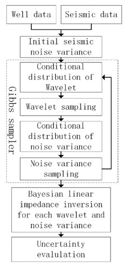
Figure 1.
Workflow of inversion.
2. Methodology
Post-stack seismic data can be regarded as:
where is the seismic record; is the logarithmic transformation of the impedance model; , is the matrix formed by the seismic wavelet; is the difference operator matrix; and is seismic noise [24,25].
Assuming that the logarithmic impedance model satisfies the Gaussian distribution of expectation vector and covariance matrix
where with defined by a second-order exponential correlation function , denotes the correlation length of . The seismic error satisfies zero-mean Gaussian distribution
when the noise covariance and wavelet matrix are known, we set , represents the wavelet, and the posterior distribution of the impedance model can be expressed as a Gaussian distribution:
where
In order to integrate the uncertainty of wavelet extraction and noise level estimation, the wavelet, noise level and their uncertainties are estimated by using well data and post-stack seismic data. The posterior distribution is expressed as
where is impedance in well data. However, it is impossible to obtain the joint posterior distribution of wavelet estimation and noise level analytically but it can be obtained by the sampling method. Some MCMC methods can be implemented, such as the Gibbs sampler and the Metropolis–Hastings algorithm [26]. These algorithms obtain a set of samples ,,…, of the posterior distribution , and is the number of samples.
In this paper, the Gibbs sampler algorithm is used to sample the joint posterior probability of wavelet and noise variance. The Gibbs sampler algorithm requires conditional distribution for every single variable given all other variables. One iteration includes sampling one element in based on the current state of other elements in . When an element is sampled it will conditionally sample another element in the current state of . That means we need to know and , which we talked about in Section 2.1 and Section 2.2. The Gibbs sampler algorithm requires multiple iterations before providing the first sample with the correct distribution. These initial iterations, called burn-in iterations, should not be used for statistical analysis. Generally, the convergence rate is difficult to estimate but it can be monitored during iteration.
For each realization , the Bayesian linear impedance inversion can obtain the corresponding posterior probability distribution. Finally, the posterior distribution of the model incorporating wavelet and noise level estimation is expressed as
The discrete form is expressed as
2.1. Conditional Distribution of Seismic Wavelet
Assuming that the seismic wavelet satisfies the Gaussian distribution with an expectation vector of and covariance matrix of
where is the length of the wavelet and . Variable is the variance of the wavelet and the covariance matrix is defined by a second-order exponential correlation function , in which the correlation length guarantees the smoothness of the estimated wavelet. We assumed and can be estimated from seismic data and well data.
The convolution in Equation (1) is reformulated as a matrix–vector multiplication,
where the matrix is obtained from the reflection coefficient calculated by the observed impedance well data.
The conditional probability distribution of the wavelet can be represented as a Gaussian distribution
where
2.2. Conditional Distribution of Seismic Noise Variance
It is assumed that the seismic error is white noise such that the noise covariance matrix can be decomposed into
where is the noise variance. In the hierarchical Bayesian model, the conjugate prior distribution for the variance of a Gaussian model is the inverse gamma distribution, which guarantees that the variance has the same prior and posterior forms [27]. Therefore, for mathematical convenience, we assumed that the unknown noise variance factor satisfies the inverse gamma distribution defined by
The expectation of inverse gamma distribution is , valid for , and the variance is , valid for . The hyper-parameters and in Equation (16) shall be defined according to prior knowledge. At this time, the conditional distribution of seismic noise variance is also inverse gamma distribution
where
3. Synthetic Model Test
We applied this method to a synthetic impedance model (black solid line in Figure 2a). The seismic data were calculated by the convolution model. The seismic wavelet was a 45 Hz Ricker wavelet. To verify the impact of seismic noise level on inversion results and uncertainties, we added Gaussian white noise with variances of 10−5, 10−4, 10−3, and 10−2, respectively, to the seismic data (Figure 2b–e).
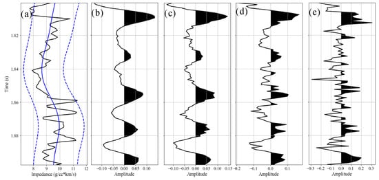
Figure 2.
Synthetic impedance model (black solid line in (a)), prior impedance model (blue solid line in (a)), 0.95 prior model interval (blue dotted lines in (a)) and seismic data with different noise levels (from (b–e) with variances of 10−5, 10−4, 10−3, and 10−2, respectively).
In the seismic inversion, the prior mean model of impedance was obtained by a low-pass filter of real impedance (blue solid line in Figure 2a). The prior covariance matrix was calculated by spatial correlation matrix with correlation length and variance obtained by statistics of the synthetic impedance model. The prior expectation vector of the seismic wavelet was 0, the variance was set as the same as the real Ricker wavelet, and the correlation length of the wavelet was set as 5 ms. The prior distribution of seismic noise variance satisfied inverse gamma distribution , which made the prior expectation of noise variance equal to 10−3. In this paper, the initial noise variance was also set to 10−3 for the Gibbs sampler in all tests with different noise levels.
The Gibbs sampler algorithm was used to sample the joint posterior probability distribution of noise level and seismic wavelet, and 5000 realizations were obtained for each test. The Bayesian linear impedance inversion was carried out respectively to obtain the posterior probability distribution of the impedance model corresponding to each pair of noise variance and seismic wavelet. Figure 3 shows the relationship between noise variance sampling results and iteration number. For different noise levels, the conditional distribution of noise variance given a wavelet realization was obtained analytically each time. Therefore, no matter how much difference between the initial noise variance and the true noise variance, the noise variance converged to the reasonable range in a few iterations, indicating that the Gibbs sampler algorithm is less affected by the initial value. We also observed that the estimated variance is slightly higher than the actual noise variance we added, which is due to the error of seismic wavelet estimation. To ensure accuracy, we set the number of burn-in iterations to 100.
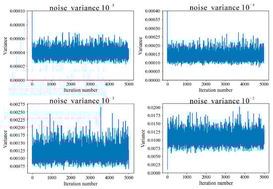
Figure 3.
The noise variance sampling versus the number of iterations.
The results of seismic wavelet extraction are shown in Figure 4. It could be observed that the accuracy and uncertainty of seismic wavelet extraction are obviously affected by the noise level. When the noise level is low, the wavelet estimation is accurate and the uncertainty is small. With the increase in the noise level, the difference between the wavelet waveform and the true Ricker wavelet becomes larger and the uncertainty increased.
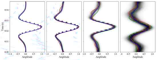
Figure 4.
The results of wavelet extraction and their probability density obtained from seismic data with different noises level (the variances are 10−5, 10−4, 10−3, and 10−2, respectively, from left to right). Blue lines are the wavelet mean model and red lines are one sample of 5000 wavelet simulations. The gray–black color represents the probability density. The green lines are the true Ricker wavelet used in synthetic seismic data.
Each wavelet and noise variance realization obtained by the Gibbs sampling was used for Bayesian linear impedance inversion to obtain the corresponding posterior probability distribution, posterior mean model and confidence interval (Figure 5). The final maximum a posteriori (MAP) solution (blue solid line) could be considered the optimal estimation of the impedance model integrated with the uncertainty of wavelet and noise level estimation [8]. The blue dotted lines indicate the 0.95 posterior confidence interval. We could observe that when the noise level is low, the inversion results are better fitted with the real model and with less uncertainty. With the increase in noise level, the inversion result deviates from the true model and the uncertainty increases. The MAP model (red lines) and the 0.95 confidence interval (green lines) corresponding to the single wavelet and noise variance realizations fluctuate around the final MAP model and confidence interval, reflecting the influence of the uncertainty of wavelet extraction and noise level estimation on the results. With the increase in noise level, the coverage range of 0.95 confidence interval of all realizations becomes wider, which means the uncertainties of the noise level estimation and the wavelet extraction have an increased impact on the uncertainty of the results.
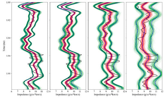
Figure 5.
Inversion results obtained from seismic data with different noises level (the variances are 10−5, 10−4, 10−3, and 10−2, respectively, from left to right). Black solid lines represent the true model, blue solid lines represent the final MAP solution of the inversion. Blue dotted lines represent the 0.95 confidence interval of the final result. Red lines represent MAP solutions corresponding to 200 of 4900 wavelet and noise variance samples.
4. Real Case
The method was applied to a 3D real case in the Gulf of Mexico containing multiple layers and a large fault. The sedimentary environment in this area is the shelf margin delta. The valid data include 3D post-stack seismic data and five well-log data (Figure 6). In our test, Wells 1 and 4 are vertical wells, which were used as known data to estimate seismic wavelet and noise levels. Wells A08, A13 and A19 are three directional wells, which were used as blind wells for algorithm verification. The seismic data include 45 inlines with an interval of 50 m and 72 crosslines with an interval of 25 m. The vertical sampling range is from 1600 ms to 2400 ms and the sampling interval is 4 ms. Through the lower gamma curve and higher resistivity curve, it could be identified that the oil-bearing sandstone is located in the Green layer, which corresponds to the low impedance characteristics (Figure 7). Therefore, the impedance inversion could be used to identify the oil-bearing sandstone.
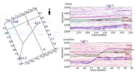
Figure 6.
Study area with well locations (left) and Seismic data (right).
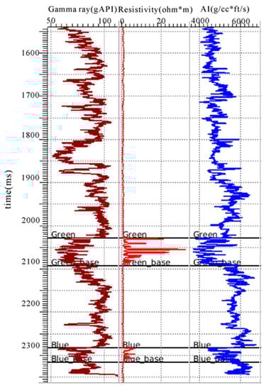
Figure 7.
Gamma-ray, resistivity and impedance curve in Well 4.
We used the horizons, fault and two vertical wells (Wells 1 and 4) to generate a prior model and estimate the prior variance of impedance. The vertical correlation length of the model was estimated as 20 ms and was used to construct a prior covariance matrix. For seismic wavelet extraction, we set the prior mean model to 0 and the spatial correlation length to 40 ms. The prior distribution of initial seismic noise variance satisfies inverse gamma distribution . We performed 5000 iterative samplings and obtained the corresponding impedance model by Bayesian linear seismic inversion.
Figure 8 shows the relationship between realizations of seismic noise variance by the Gibbs sampling and the iteration number. Similar to the result of the synthesis model, the burn-in iteration is fast and stable. We also set the number of burn-in iterations to 100 and counted the last 4900 samples. It could be seen that the final noise variance ranges from 1.5 to 2, and the average is approximately 1.8. The MAP model and one wavelet realization by Gibbs sampling are shown in Figure 9. The gray–black color represents the posterior probability density of wavelet extraction. The prior model used in Bayesian linear impedance inversion, the final posterior MAP model and the MAP models corresponding to each pair of noise variance and wavelet realizations are shown in Figure 10. The results could clearly see the low impedance area in the target layer. We verified the inversion results by the three blind wells (Figure 11). The final posterior MAP models (blue solid lines) at well locations are well-matched with well-log data, which shows the correctness of our method. The 0.95 confidence intervals of the final posterior models (blue dotted lines) show the uncertainty of the impedance model. The red lines and green lines are the MAP models and 0.95 confidence intervals corresponding to 200 of 4900 noise variance and wavelet realizations. Their coverage indicates the uncertainty caused by wavelet extraction and noise level estimation.
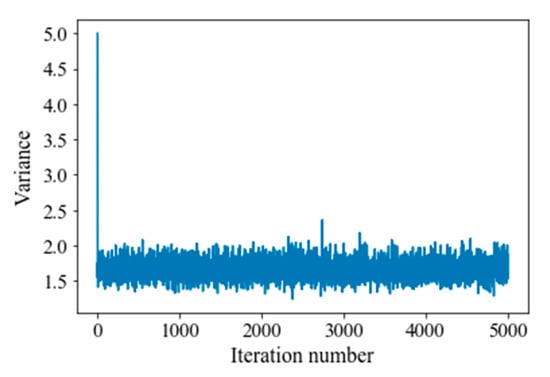
Figure 8.
The seismic noise variance sampling versus the iteration number.
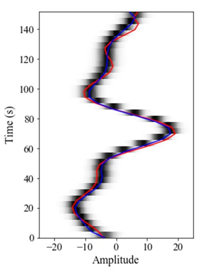
Figure 9.
The results of wavelet extraction. Blue line is the MAP solution of wavelet extraction and red line is one wavelet realization drawn by Gibbs sampling. The gray–black color represents the posterior probability density.
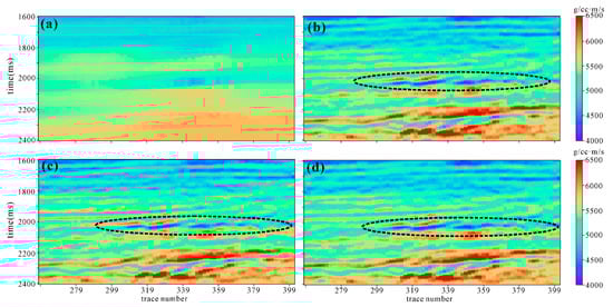
Figure 10.
The 2D cross-section of inversion results: (a) prior mean model, (b) final posterior MAP model, (c,d) MAP models for 2 of 4900 realizations of wavelet and noise variance.
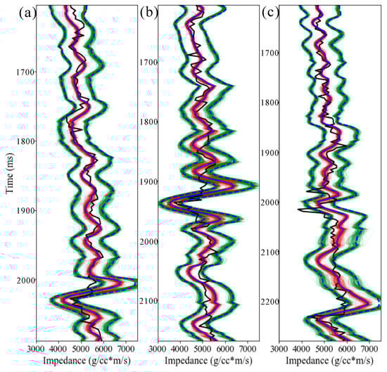
Figure 11.
Inversion results at well (a) A08, (b) A13 and (c) A19. The black solid lines represent well-log data. The blue solid lines represent the final MAP model and the blue dotted lines represent the 0.95 confidence interval. The red lines represent the MAP model corresponding to 200 of 4900 wavelet and noise variance realizations.
The CPU of the computer we used for this 3D experiment is an Intel Core i7-8700 (3.20 GHz). It took about an hour to obtain the 5000 realizations. Because of the linear assumption and the specified distribution assumption of model parameters, the calculation efficiency is high. For larger models, inversion could still be performed efficiently using computers with more cores or GPU acceleration.
5. Conclusions
In this paper, a Bayesian linear inversion method of seismic impedance is proposed, which combines the uncertainty of the data noise level estimation and seismic wavelet extraction. The method first obtains the estimation of seismic data noise level, seismic wavelet and their uncertainty through the analytical Bayesian method and Gibbs sampler, and then integrates this uncertainty into seismic impedance Bayesian linear inversion to obtain the impedance model and uncertainty evaluation. The synthetic model and data tests with different noise levels show that the method in this paper could obtain an accurate estimation of noise levels and their uncertainties. This method provides uncertainty evaluation not only for the impedance model but also for noise level estimation and wavelet extraction. Finally, the method is successfully applied to the real case data, which further verifies the effectiveness of the algorithm. This method is carried out under the assumption that the model satisfies the linear relation and the parameters satisfy the specified distribution, which makes the method more efficient. However, when facing more complex media, such as anisotropic models or the assumptions not being exactly in line with reality, this method will lose some accuracy.
In addition to the uncertainty of seismic noise level estimation and wavelet extraction, there are uncertainty factors in the observed error of well-log data, time error of well seismic calibration, seismic wavelet variance, autocorrelation length and so on. This paper does not carry out the corresponding research but this method can be extended similarly.
Author Contributions
Conceptualization, X.Y. and P.Z.; methodology, X.Y. and N.M.; validation, X.Y., P.Z. and N.M.; formal analysis, X.Y.; investigation, X.Y.; resources, X.Y.; data curation, X.Y.; writing—original draft preparation, X.Y.; writing—review and editing, X.Y., N.M. and P.Z.; visualization, X.Y.; supervision, N.M. and P.Z.; project administration, X.Y.; funding acquisition, X.Y. All authors have read and agreed to the published version of the manuscript.
Funding
This research was funded by the National Natural Science Foundation of China, grant number 42204120.
Data Availability Statement
Not applicable.
Conflicts of Interest
The authors declare no conflict of interest. The funders had no role in the design of the study; in the collection, analyses, or interpretation of data; in the writing of the manuscript; or in the decision to publish the results.
References
- Cooke, D.A.; Schneider, W.A. Generalized linear inversion of reflection seismic data. Geophysics 1983, 48, 665–676. [Google Scholar] [CrossRef]
- Oldenburg, D.W.; Scheuer, T.; Levy, S. Recovery of the acoustic impedance from reflection seismograms. Geophysics 1983, 48, 1318–1337. [Google Scholar] [CrossRef]
- Dai, R.; Yin, C.; Peng, D. Elastic Impedance Simultaneous Inversion for Multiple Partial Angle Stack Seismic Data with Joint Sparse Constraint. Minerals 2022, 12, 664. [Google Scholar] [CrossRef]
- Sen, M.K.; Stoffa, P.L. Nonlinear one-dimensional seismic waveform inversion using simulated annealing. Geophysics 1991, 56, 1624–1638. [Google Scholar] [CrossRef]
- Mallick, S. Some practical aspects of prestack waveform inversion using a genetic algorithm: An example from the east Texas Woodbine gas sand. Geophysics 1999, 64, 326–336. [Google Scholar] [CrossRef]
- Tarantola, A. Inverse Problem Theory and Methods for Model Parameter Estimation; Society for Industrial and Applied Mathematics: Philadelphia, PA, USA, 2005. [Google Scholar]
- Bosch, M.; Mukerji, T.; Gonzalez, E.F. Seismic inversion for reservoir properties combining statistical rock physics and geostatistics: A review. Geophysics 2010, 75, 75A165–175A176. [Google Scholar] [CrossRef]
- Buland, A.; Omre, H. Bayesian linearized AVO inversion. Geophysics 2003, 68, 185–198. [Google Scholar] [CrossRef]
- Grana, D.; Fjeldstad, T.; Omre, H. Bayesian Gaussian Mixture Linear Inversion for Geophysical Inverse Problems. Math. Geosci. 2017, 49, 493–515. [Google Scholar] [CrossRef]
- Yang, X.; Zhu, P. Stochastic seismic inversion based on an improved local gradual deformation method. Comput. Geosci. 2017, 109, 75–86. [Google Scholar] [CrossRef]
- de Figueiredo, L.P.; Grana, D.; Roisenberg, M.; Rodrigues, B.B. Gaussian mixture Markov chain Monte Carlo method for linear seismic inversion. Geophysics 2019, 84, R463–R476. [Google Scholar] [CrossRef]
- Scales, J.A.; Tenorio, L. Prior information and uncertainty in inverse problems. Geophysics 2001, 66, 372–698. [Google Scholar] [CrossRef]
- Park, H.; Scheidt, C.; Fenwick, D.; Boucher, A.; Caers, J. History matching and uncertainty quantification of facies models with multiple geological interpretations. Comput. Geosci. 2013, 17, 609–621. [Google Scholar] [CrossRef]
- Scheidt, C.; Jeong, C.; Mukerji, T.; Caers, J. Probabilistic falsification of prior geologic uncertainty with seismic amplitude data: Application to a turbidite reservoir case. Geophysics 2015, 80, M12–M89. [Google Scholar] [CrossRef]
- Hadiloo, S.; Radad, M.; Mirzaei, S.; Foomezhi, M. Seismic Facies Analysis by ANFIS and Fuzzy Clustering Methods to Extract Channel Patterns. In Proceedings of the 79th EAGE Conference and Exhibition, Paris, France, 12–15 June 2017; pp. 1–5. [Google Scholar]
- Azevedo, L.; Demyanov, V. Multi-scale uncertainty assessment in geostatistical seismic inversion. Geophysics 2019, 84, R355–R369. [Google Scholar] [CrossRef]
- Grana, D. Bayesian petroelastic inversion with multiple prior modelsBayesian inversion with multiple priors. Geophysics 2020, 85, M57–M71. [Google Scholar] [CrossRef]
- Talarico, E.C.S.; Grana, D.; de Figueiredo, L.P.; Pesco, S. Uncertainty quantification in seismic facies inversion. Geophysics 2020, 85, M43–M56. [Google Scholar] [CrossRef]
- Yang, X.; Mao, N.; Zhu, P.; Xiao, D. Two-level uncertainty assessment in stochastic seismic inversion based on gradual deformation method. Geophysics 2020, 85, M33–M42. [Google Scholar] [CrossRef]
- Liu, M.; Grana, D.; de Figueiredo, L.P. Uncertainty quantification in stochastic inversion with dimensionality reduction using variational autoencoder. Geophysics 2022, 87, M43–M58. [Google Scholar] [CrossRef]
- Chen, T.; Wang, Y.; Li, K.; Cai, H.; Yu, G.; Hu, G. A prestack seismic inversion method constrained by facies-controlled sedimentary structural features. Geophysics 2022, 88, 1–102. [Google Scholar] [CrossRef]
- Kolbjørnsen, O.; Buland, A.; Hauge, R.; Røe, P.; Ndingwan, A.O.; Aker, E. Bayesian seismic inversion for stratigraphic horizon, lithology, and fluid prediction. Geophysics 2020, 85, R207–R221. [Google Scholar] [CrossRef]
- Thore, P. Uncertainty in seismic inversion:What really matters? Lead. Edge 2015, 34, 1000–1002, 1004. [Google Scholar] [CrossRef]
- Dai, R.; Yang, J. An alternative method based on region fusion to solve L0-norm constrained sparse seismic inversion. Explor. Geophys. 2021, 52, 624–632. [Google Scholar] [CrossRef]
- Yang, J.; Yin, C.; Dai, R.; Yang, S.; Zhang, F. Seismic impedance inversion via L0 gradient minimisation. Explor. Geophys. 2019, 50, 575–582. [Google Scholar] [CrossRef]
- Chen, M.; Shao, Q.; Ibrahim, J.G. Monte Carlo Methods in Bayesian Computation, 1st ed.; Springer: New York, NY, USA, 2000. [Google Scholar]
- Robert, C.P. The Bayesian Choice, 2nd ed.; Springer: New York, NY, USA, 2007. [Google Scholar]


Disclaimer/Publisher’s Note: The statements, opinions and data contained in all publications are solely those of the individual author(s) and contributor(s) and not of MDPI and/or the editor(s). MDPI and/or the editor(s) disclaim responsibility for any injury to people or property resulting from any ideas, methods, instructions or products referred to in the content. |
© 2022 by the authors. Licensee MDPI, Basel, Switzerland. This article is an open access article distributed under the terms and conditions of the Creative Commons Attribution (CC BY) license (https://creativecommons.org/licenses/by/4.0/).