Magnetotelluric Responses of an Anisotropic 1-D Earth with a Layer of Exponentially Varying Conductivity

Abstract

The magnetotelluric (MT) sounding of a layered Earth model involving a transitional layer has been widely studied, and MT responses of the model with dipping anisotropic conductivity have also been treated. However, a model incorporating both a transitional layer and dipping anisotropy has seldom been considered. The analytical solution of such a geoelectrical model including three layers was derived in this study. The middle layer was a transitional layer with conductivity exponentially varying with depth, which was covered by a homogeneous layer and underlaid by a dipping anisotropic half-space. The electromagnetic (EM) fields in the transitional layer were explicitly solved with modified Bessel functions. The surface impedance was calculated recursively. The dependence of the apparent resistivity and impedance phase as well as the EM fields on different model parameters were investigated in detail. We believe that our analytical solution provides a useful complement to the theory of the one-dimensional (1D) inversion and interpretation based on the layered model with fixed conductivity.

1. Introduction

The magnetotelluric (MT) [1,2,3] method is a passive geophysical exploration technique for determining the subsurface conductivity structure using natural electromagnetic (EM) fields. With advances in computer technology and numerical techniques, it is now possible to calculate the MT responses of various complex models in two dimensions (2D) and three dimensions (3D) by numerical modelling; thus, many programs have been developed [4,5,6,7,8,9,10,11,12,13,14,15,16,17,18,19]. However, although a number of 2D and 3D numerical simulation codes have been developed and applied in many aspects related to MT research, studies on the analytical responses over a one-dimensional (1D) Earth model still have a certain degree of importance in the application of MT techniques, especially in some special circumstances, for example, on the ocean bottom, where, sometimes, not enough MT data are available to conduct 2D or 3D studies, and 1D inversion and interpretation is a necessary technique [20]. Furthermore, a 1D solution may be presented as a technical appendix to a publication presenting a 3D solver, since it is very useful when developing 3D solvers and verifying their accuracy. Additionally, 1D MT is still applied to probe some simple structures such as basin depth [21] and geothermal fields [22,23,24], and it is also used to understand EM wave propagation in the Earth [25].

Most of the publications on the 1D analytical solutions of MT responses appeared in the 1970s–1980s or earlier. The models considered in these publications may be categorized into two groups: those with sharp boundaries [26,27,28,29,30,31] and those with transitional boundaries [32,33,34,35,36,37]. In the former case, the model is composed of several layers with fixed conductivity; while in the latter case, the model includes at least one layer in which the conductivity varies with depth. From the perspective of practical observation, a number of resistivity well-logging analyses [38,39,40] have advocated that the boundaries between layers are transitional in nature rather than sharp. Therefore, studies of MT responses to 1D transitional models are important and necessary.

Some authors have reported analytical solutions to the MT fields of 1D transitional models. For instance, Mallick [32] and Kao and Rankin [34] examined the MT responses of an inhomogeneous layered Earth of conductivity linearly varying with depth. Berdichevsky et al. [41] considered the MT responses of models of resistivity exponentially decreasing with depth. Banerjee et al. [37] reported the apparent resistivity of a multilayered Earth with a layer having exponential variation in the conductivity. Kao [35] considered the MT fields of a vertical inhomogeneous model of resistivity varying linearly with depth. Kao [36] also presented the MT responses to a 1D model with the conductivity varying exponentially as a function of depth. Kim and Lee [42] investigated the response of a layered Earth of resistivity exponentially varying with depth. Pal [43] examined the MT responses over a 1D Earth with a nonmonotonic resistivity distribution in a transitional layer. Additionally, Berdichevsky and Dmitriev [44] summarized the analytical solutions of two special cases of gradient models, i.e., the Dmitriev–Kao model [36,41] and the Kato–Kikuchi model [45], which are characterized by exponentially varying conductivity with depth. Qin and Yang [46] calculated the MT responses over a layered model containing two transitional layers.

However, these previously mentioned models did not involve anisotropy. There have been some studies in which the model involved electrical anisotropy. For example, Negi and Saraf [47] reported the MT sounding of a layered model with a transitional layer underlaid by a dipping anisotropic half-space in which the conductivity in the transition layer varied linearly with depth. Kovacikova and Pek [48] presented generalized Riccati equations for 1D MT impedances of electrical anisotropic structures. Recently, Qin et al. [49] published the MT responses of a 1D resistivity structure model involving anisotropic transitional layers.

In this study, we extended the work of Negi and Saraf [47] to a case where the conductivity varied exponentially with depth in the transitional layer. Although this model is a very specific setting, it is still necessary and important to consider. The first layer may represent the shallow sediment layer. The transitional layer can describe a frozen surface layer [50] or the zone of weathered rock [51]. For the bottom layer with uniaxial anisotropy, the plane of anisotropy makes an angle with the horizontal interface between the transitional layer and the basement; such an interface may behave as a plane of unconformity between two sedimentary strata (a typical stratigraphic trap, which is favourable for the accumulation of oil), therefore, an analysis of the MT responses to such a model is expected to be beneficial for oil exploration [52]. Moreover, it is well known that the transitional layer can be approximately equivalent to numbers of thin layers that have fixed conductivities with depth [46,53], and further numerical approaches can be adopted to obtain the MT responses. However, as stated by Chlamtac and Abramovici [50], when the calculation is considered in inverse problems, the number of parameters to be determined using this three-layer model is largely fewer than that using a stack of thin layers and thus simplifies the problem.

The rest of this work is arranged as follows: the model and its MT responses are demonstrated in Section 2. After that, the validation of the algorithm is presented in Section 3. Next, in Section 4, the variation in the MT responses with the model parameters is illustrated. Finally, the conclusions are given in Section 5.

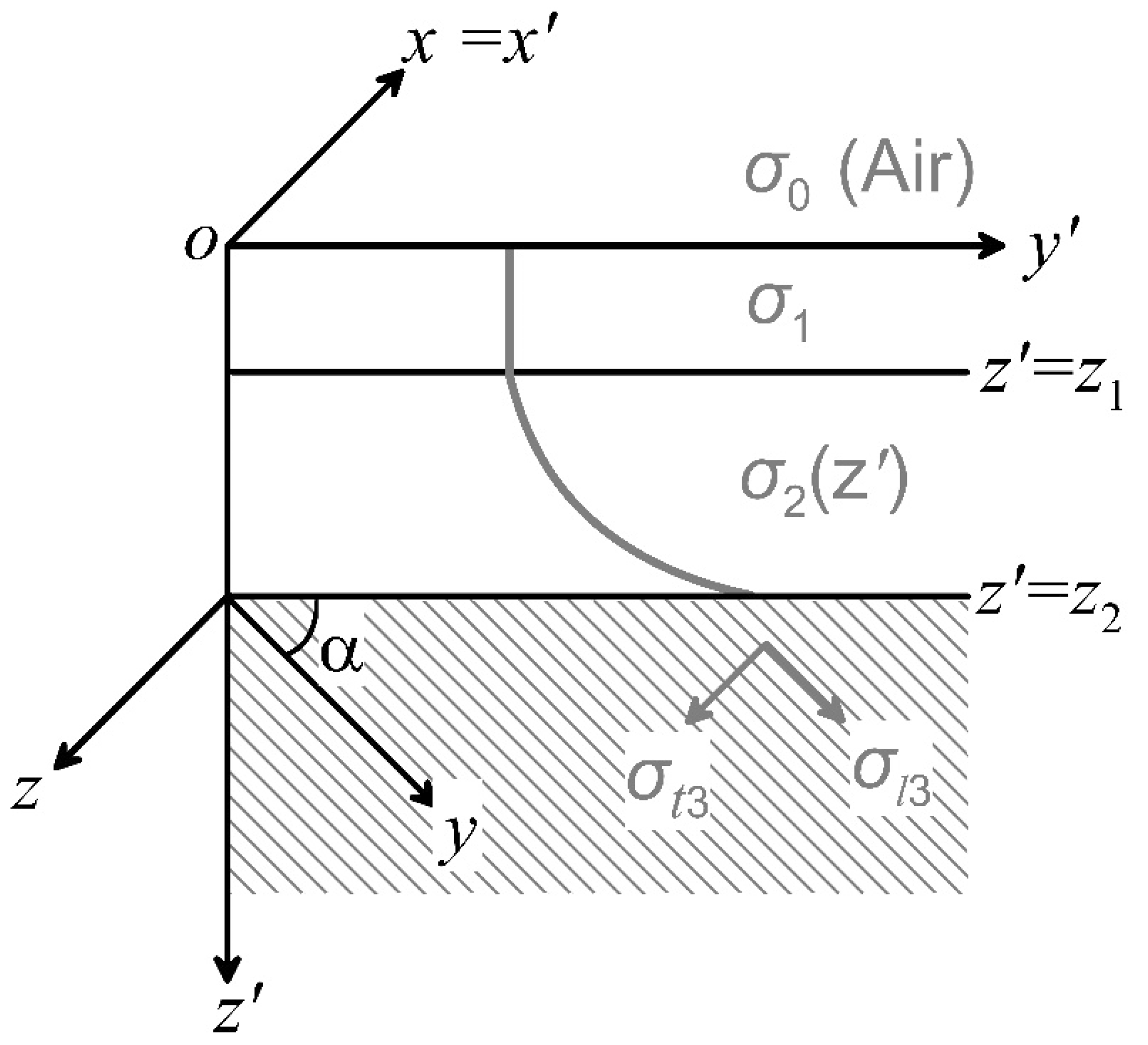
2. Model and Formulations

2.1. The Vertical Inhomogeneous and Anisotropic Model

For the problem considered in the following texts, a plane EM wave with the time factor $e^{i\omega t}$ ($\omega$ and $t$ are the angular frequency and time, respectively; $i$ is the imaginary unit and $i=\sqrt{-1}$) is assumed. The 1D layered model to be treated is shown in Figure 1. The model is composed of two different media: the isotropic medium (the first and second layers) and the anisotropic medium in the base (the third layer). In addition, the second layer is a transitional layer with conductivity that varies exponentially with depth. To solve the induction problem in this work, we set up two different coordinate systems: one is $\mathit{\text{o-x}}{}^{\prime }{y}^{\prime }{z}^{\prime }$ (a Cartesian coordinate system) for the isotropic media, and the other is $\mathit{\text{o-xyz}}$ for the anisotropic medium in the third layer (a principal axes coordinate system). Just to make the model clear, the coordinate systems are represented by black axes and the conductivity parameters are marked by grey axes.

For simplicity, the problem is treated in Cartesian coordinates, in which the horizontal electric field component $E_{y^{\prime }}$ and orthogonal horizontal magnetic field $H_{x^{\prime }}$ are typically to be solved.

The electrical conductivity in the middle layer is assumed to be written as:

$${\sigma }_2\left(z{}^{\prime }\right)={\sigma }_1{e}^{q\left(z{}^{\prime }-z_1\right)}$$

(1)

where $z_1$ indicates the depth of the interface between the top and middle layers, and $q$ in the exponential power is the rate of the change in conductivity, which may be defined by

$$q=\ln [{\sigma }_{l3}/({\sigma }_1{\beta }^2)]/\left(z_2-z_1\right)$$

(2)

where ${\beta }^2 = 1+\left({\lambda }^2-1\right){\sin }^2\alpha$, $\lambda ={\left({\sigma }_{l3}/{\sigma }_{t3}\right)}^{1/2}$ is the coefficient of anisotropy, the longitudinal conductivity ${\sigma }_{l3}$ is parallel to the axis $y$, the transverse conductivity ${\sigma }_{t3}$ is parallel to the axis $z$, and $z_2$ is the depth of the lower boundary of the second layer from the surface of the Earth.

Due to the different characteristics of the conductivity in the three layers, Maxwell’s equations must be solved in the three layers to calculate the EM fields.

2.2. The EM Fields in the Top Layer

The displacement current is usually ignored for MT soundings; thus, the Helmholtz equation to be satisfied in the isotropic layer may be written as [47,54,55]:

$$\frac{d^2{E}_{y{}^{\prime }1}}{d{z^{\prime }}^2}-k_1^2{E}_{y{}^{\prime }1}=0$$

(3)

where $k_1=\sqrt{i\omega \mu {\sigma }_1}$ defines the propagation constant of the EM wave, $\mu$ is the magnetic permeability and $E_{y{}^{\prime }1}$ is the horizontal electric field in the top layer.

The general solution to Equation (3) is given by the following formula [56]:

$$E_{y{}^{\prime }1}=A{e}^{-k_1{z}^{\prime }}+B{e}^{k_1{z}^{\prime }}$$

(4)

where $A$ and $B$ are undetermined coefficients to be found by applying the boundary conditions.

Once the electric field has been obtained, the horizontal magnetic field component can be easily obtained using the following formula from Maxwell’s equations:

$$H_{x^{\prime }1}=\frac{1}{i\omega \mu }\frac{\partial E_{y{}^{\prime }1}}{\partial z^{\prime }}$$

(5)

By combining Equations (4) and (5), the horizontal magnetic field component is given by:

$$H_{x^{\prime }1}=\frac{k_1}{i\omega \mu }\left(-A{e}^{-k_1{z}^{\prime }}+B{e}^{k_1{z}^{\prime }}\right)$$

(6)

2.3. The EM Fields in the Middle Layer

The Helmholtz’s equation governing EM induction in the middle layer is expressed as:

$$\frac{d^2{E}_{y{}^{\prime }2}}{d{z^{\prime }}^2}-k_2^2{E}_{y{}^{\prime }2}=0$$

(7)

where $k_2=\sqrt{i\omega \mu {\sigma }_2\left(z^{\prime }\right)}$ is the propagation constant (varying with the depth) in the region of 2 and $E_{y{}^{\prime }2}$ represents the corresponding horizontal electric field component.

Substitution of Equation (1) into (7) yields:

$$\frac{d^2{E}_{y{}^{\prime }2}}{d{z^{\prime }}^2}-i\omega \mu {\sigma }_1{e}^{q\left(z^{\prime }-z_1\right)}{E}_{y{}^{\prime }2}=0$$

(8)

Now, we introduce a new variable $\gamma$, which is defined as:

$$\gamma =2\sqrt{i\omega \mu {\sigma }_1{e}^{q\left(z^{\prime }-z_1\right)}}/q$$

(9)

Thus, the first-order derivative of $\gamma$ is obtained from Equation (9):

$$\frac{d\gamma }{d{z}^{\prime }}=\sqrt{i\omega \mu {\sigma }_1{e}^{q\left(z^{\prime }-z_1\right)}}$$

(10)

Subsequently, combining Equations (8)–(10) yields a second-order differential equation of $E_{y{}^{\prime }2}$ for the variable $\gamma$:

$$\frac{d^2{E}_{y{}^{\prime }2}}{d{\gamma }^2}+\frac{1}{\gamma }\frac{d{E}_{y{}^{\prime }2}}{d\gamma }-E_{y{}^{\prime }2}=0$$

(11)

Clearly, Equation (11) is a modified Bessel equation of zero order, and its general solution has the following form [57]:

$$E_{y{}^{\prime }2}=C{I}_0\left(\gamma \right)+D{K}_0\left(\gamma \right)$$

(12)

where $I_0\left(\gamma \right)$ and $K_0\left(\gamma \right)$ are the modified Bessel functions of the first and second type of order zero, respectively, and $C$ and $D$ are undetermined coefficients to be evaluated by applying the boundary conditions.

Next, the horizontal magnetic field component $H_{x{}^{\prime }2}$ is examined by Equation (12) with the help of $I_0^{\prime }\left(\gamma \right)=I_1\left(\gamma \right)$ and $K_0^{\prime }\left(\gamma \right)=-K_1\left(\gamma \right)$, and the derivative of $E_{y{}^{\prime }2}$ with respect to $z^{\prime }$ can be written as a function of $\gamma$ thanks to Equation (10):

$$\begin{array}{l}{H}_{x{}^{\prime }2}=\frac{1}{i\omega \mu }\frac{\partial E_{y{}^{\prime }2}}{\partial z^{\prime }}=\frac{1}{i\omega \mu }\frac{d{E}_{y{}^{\prime }2}}{d\gamma }\sqrt{i\omega \mu {\sigma }_1{e}^{q\left(z^{\prime }-z_1\right)}}\\ =\frac{\sqrt{i\omega \mu {\sigma }_1{e}^{q\left(z^{\prime }-z_1\right)}}}{i\omega \mu }\left[C{I}_1\left(\gamma \right)-D{K}_1\left(\gamma \right)\right]\end{array}$$

(13)

2.4. The EM Fields in the Bottom Layer

The EM fields in a dipping anisotropic medium have been previously investigated [52,58]; these results were used in this study. Thus, the horizontal magnetic field component $H_{x{}^{\prime }3}$ in the bottom layer is given by the following expression:

$$H_{x3}=H_{x{}^{\prime }3}=F{e}^{-k_3{z}^{\prime }}=F{e}^{-k_3\left(z\cos \alpha +y\sin \alpha \right)}$$

(14)

where $k_3=\sqrt{i\omega \mu {\sigma }_{l3}/{\beta }^2}$ is the propagation constant in the bottom layer, and $F$ is an undetermined coefficient to be estimated by applying boundary conditions.

From Maxwell’s equation, the horizontal electric field can be related to the horizontal magnetic component in the dipping anisotropic medium via the following expressions [52,58]

$$\{\begin{array}{l}\frac{\partial H_{x3}}{\partial z}={\sigma }_{l3}{E}_{y3}\\ \frac{\partial H_{x3}}{\partial y}=-{\sigma }_{t3}{E}_{z3}\end{array}$$

(15)

Substitution of Equation (14) into (15) gives the horizontal and vertical electric components in the bottom layer:

$$\{\begin{array}{l}{E}_{y3}=-\frac{k_3\cos \alpha }{{\sigma }_{l3}}F{e}^{-k_3\left(z\cos \alpha +y\sin \alpha \right)}\\ E_{z3}=\frac{k_3\sin \alpha }{{\sigma }_{t3}}F{e}^{-k_3\left(z\cos \alpha +y\sin \alpha \right)}\end{array}$$

(16)

Finally, the horizontal electric component $E_{y{}^{\prime }3}$ needs to be determined in the Cartesian coordinate system; therefore, a relationship should be established between the Cartesian coordinate system and the principal axes coordinate system. This relationship may be easily seen in Figure 1; that is, $z{}^{\prime }=z\cos \alpha +y\sin \alpha$. Hence, the horizontal electric component $E_{y{}^{\prime }2}$ may be written as:

$$\begin{array}{l}{E}_{y{}^{\prime }3}=E_{y3}\cos \alpha -E_{z3}\sin \alpha \\ \begin{array}{cc}& =\end{array}\frac{-k_3{\beta }^2}{{\sigma }_{l3}}F{e}^{-k_3\left(z\cos \alpha +y\sin \alpha \right)}\\ \begin{array}{cc}& =\end{array}\frac{-k_3{\beta }^2}{{\sigma }_{l3}}F{e}^{-k_3{z}^{\prime }}\end{array}$$

(17)

2.5. Evaluation of Undetermined Coefficients

The electric and magnetic fields in the three layers of the model in Figure 1 have been explicitly examined with several undetermined coefficients (i.e., A, B, C, and D), which were evaluated using the boundary conditions at $z^{\prime }=z_1$ and $z^{\prime }=z_2$. The equivalence of the electric and magnetic fields at the two interfaces may be written as follows:

$$\{\begin{array}{l}{E}_{y{}^{\prime }1}=E_{y{}^{\prime }2}\\ H_{x^{\prime }1}=H_{x^{\prime }2}\\ E_{y{}^{\prime }2}=E_{y{}^{\prime }3}\\ H_{x^{\prime }2}=H_{x^{\prime }3}\end{array}$$

(18)

Substitution of Equations (4), (6), (12)–(14) and (17) into Equation (18) yields:

$$\{\begin{array}{l}A{e}^{-k_1{z}_1}+B{e}^{k_1{z}_1}=C{I}_0\left({\gamma }_1\right)+D{K}_0\left({\gamma }_1\right)\\ -A{e}^{-k_1{z}_1}+B{e}^{k_1{z}_1}=C{I}_1\left({\gamma }_1\right)-D{K}_1\left({\gamma }_1\right)\\ C{I}_0\left({\gamma }_2\right)+D{K}_0\left({\gamma }_2\right)=NF{e}^{-k_3{z}_2}\\ U\left[C{I}_1\left({\gamma }_2\right)-D{K}_1\left({\gamma }_2\right)\right]=F{e}^{-k_3{z}_2}\end{array}$$

(19)

where ${\gamma }_1={\gamma |}_{z=z_1}=2\sqrt{i\omega \mu {\sigma }_1}/q$, ${\gamma }_2={\gamma |}_{z=z_2}=2\sqrt{i\omega \mu {\sigma }_1{e}^{p\left(z_2-z_1\right)}}/q$, $N=-\frac{k_3{\beta }^2}{{\sigma }_{l3}}$ and $U=\sqrt{\frac{{\sigma }_1{e}^{q\left(z_2-z_1\right)}}{i\omega \mu }}$.

The relationships of different unknown coefficients may be obtained from Equation (19) (see the details in Appendix A).

2.6. Apparent Resistivity and Impedance Phase

Once the relationship of the EM fields at the surface of the model has been obtained, the surface impedance can be immediately deduced from the following expression:

$${Z|}_{{}_{z^{\prime }=0}}={\frac{E_{y{}^{\prime }1}}{H_{x^{\prime }1}}|}_{{}_{z^{\prime }=0}}=\frac{i\omega \mu }{k_1}\frac{1+A/B}{1-A/B}$$

(20)

where $A/B$ is recursively solved from Equation (19) (see Appendix A for details).

Furthermore, the apparent resistivity ${\rho }_a$ and the impedance phase $\phi$ can be examined using the following expressions:

$$\{\begin{array}{l}{\rho }_a={\left|Z\right|}^2/\omega \mu \\ \phi ={\tan }^{-1}\left(Z_{\mathrm{Im}}/Z_{\mathrm{Re}}\right)\end{array}$$

(21)

where $Z_{\mathrm{Im}}$ and $Z_{\mathrm{Re}}$ represent the imaginary and real parts of the surface impedance, respectively.

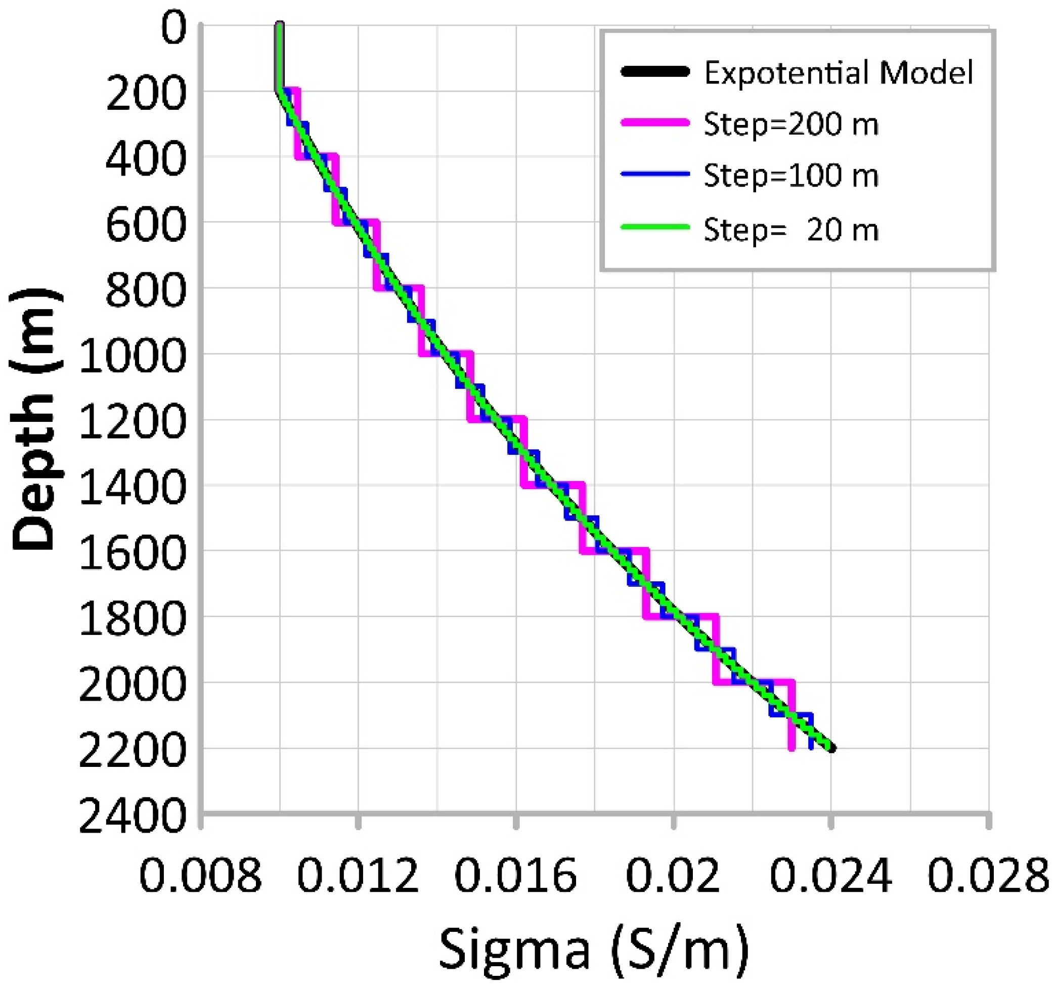
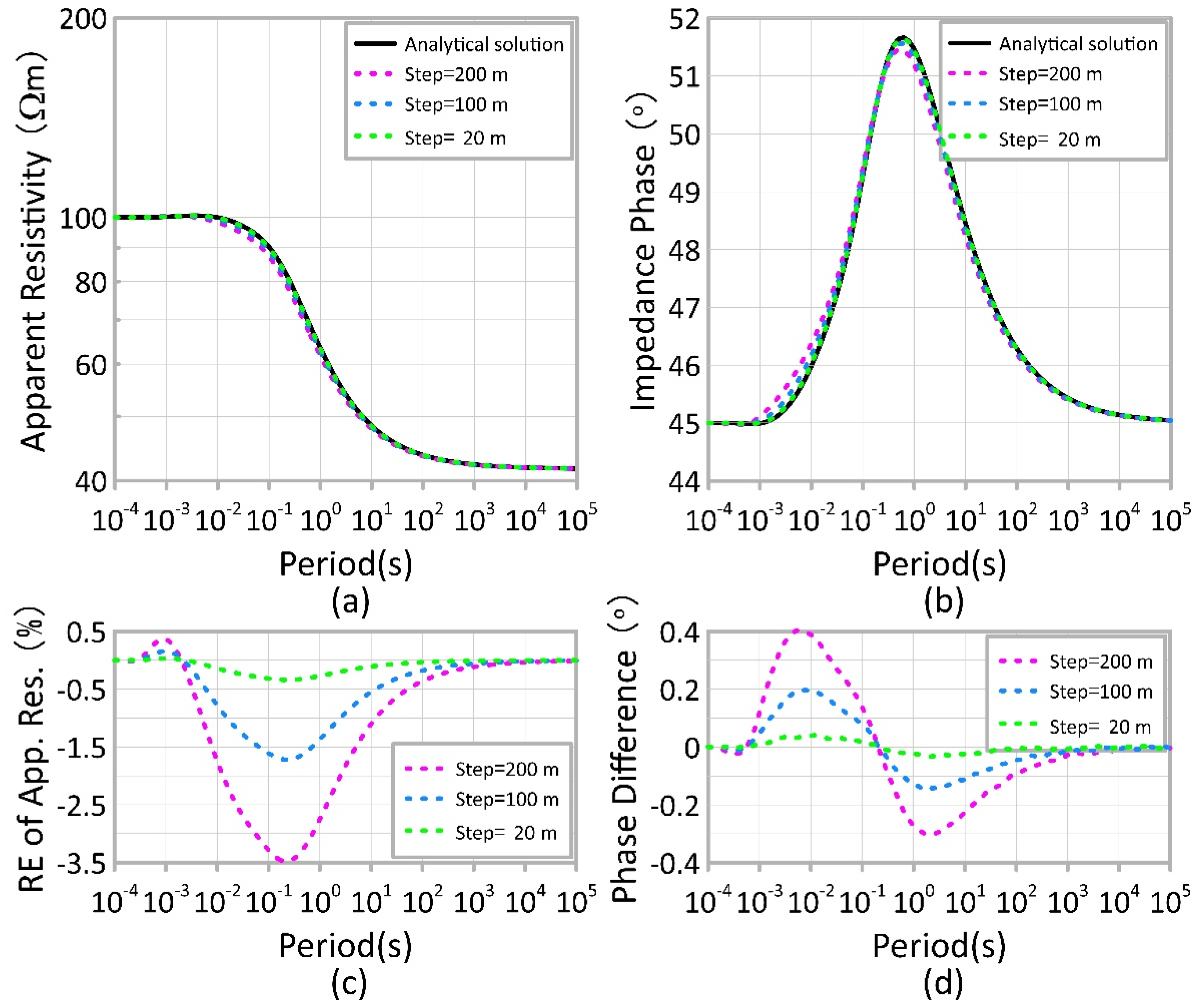
3. Validation of the Method

The algorithm presented in the previous section was validated by comparing the apparent resistivity and impedance phase calculated by the method in this work for the 1D model shown in Figure 1 (called the exponential model hereinafter) and results were obtained using the program code Z1ANIS.FOR provided by Pek and Santos [59] (referred to as Pek1DAniCode in the following text; see Appendix B for details) for homogeneous multilayer approximation models (hereafter called the stair-step model). The model parameters of the exponential model are as follows: ${\sigma }_1 = 0.01 \mathrm{S}/\mathrm{m}$, ${\sigma }_{l3} = 0.02 \mathrm{S}/\mathrm{m}$, ${\sigma }_{t3} = 0.06 \mathrm{S}/\mathrm{m}$, $z_1 = 200 \mathrm{m}$, $z_2 = 2200 \mathrm{m}$, and $\alpha = 30°$. To evaluate the validity of the analytical solution in this study, three stair-step models with steps of 200, 100 and 20 m were designed to approximate the transitional layer in the exponential model. The first and second layers are shown in Figure 2, where the black solid curve represents the exponential model considered in this study, and the magenta, blue and green lines represent the stair-step models with a step of 200, 100 and 20 m, respectively. For the stair-step models, the conductivities of thin layers within the depth of the middle layer in the exponential model were calculated using Equation (1).

For the given model, the apparent resistivity and impedance phase were computed by the method described in Section 2 and by Pek1DAniCode, respectively. The corresponding results are shown in Figure 3. The apparent resistivity of the exponential model is shown by the black solid curve in Figure 3a, while the apparent resistivity of the stair-step models with steps of 200, 100 and 20 m are indicated by magenta, blue and green dashed curves, respectively. Figure 3b shows the impedance phase for the exponential model (black curve) and stair-step models (magenta, blue and green curves).

To evaluate the accuracy of the algorithm in this work, the relative error (RE) of the apparent resistivity of the different models was introduced, and the phase difference (PD) of the models was also evaluated. The formulas used to calculate RE and PD are as follows:

$$\{\begin{array}{l}RE=\frac{{\rho }_{as}-{\rho }_{ss}}{{\rho }_{as}}\times 100\%\\ PD={\phi }_{as}-{\phi }_{ss}\end{array}$$

(22)

where ${\rho }_{as}$ and ${\phi }_{as}$ represent the apparent resistivity and impedance of the analytic solution, respectively, and ${\rho }_{ss}$ and ${\phi }_{ss}$ are the apparent resistivity and impedance of the step-stair models calculated by Pek1DAniCode, respectively.

The RE of the apparent resistivity for the stair-step models with respect to the ones for the exponential model were computed using Equation (22), and the corresponding results are indicated by the magenta, blue and green dashed curves in Figure 3c. The maximum value of RE in the apparent resistivity was approximately −3.5% when the step was 200 m (i.e., the thickness of layers approximating the transitional layer was 200 m), while it decreased to less than 0.5% when the step decreased to 20 m. The phase difference (PD) between the results for the stair-step models and those for the exponential model were also calculated by Equation (22), and the resulting values are represented by the magenta, blue and green dashed curves in Figure 3d. The maximum value of PD was approximately 0.4° when the step was 200 m, while it decreased to less than 0.05° when the step was reduced to 20 m.

Thus, the comparison in Figure 3 clearly shows that the apparent resistivity and impedance phase for the stair-step model obtained with Pek1DAniCode asymptotically converge to the analytical solution of the exponential model with an increasing number of layers (decreasing thickness) approximating the transitional layer. Therefore, the algorithm presented in this study has been validated.

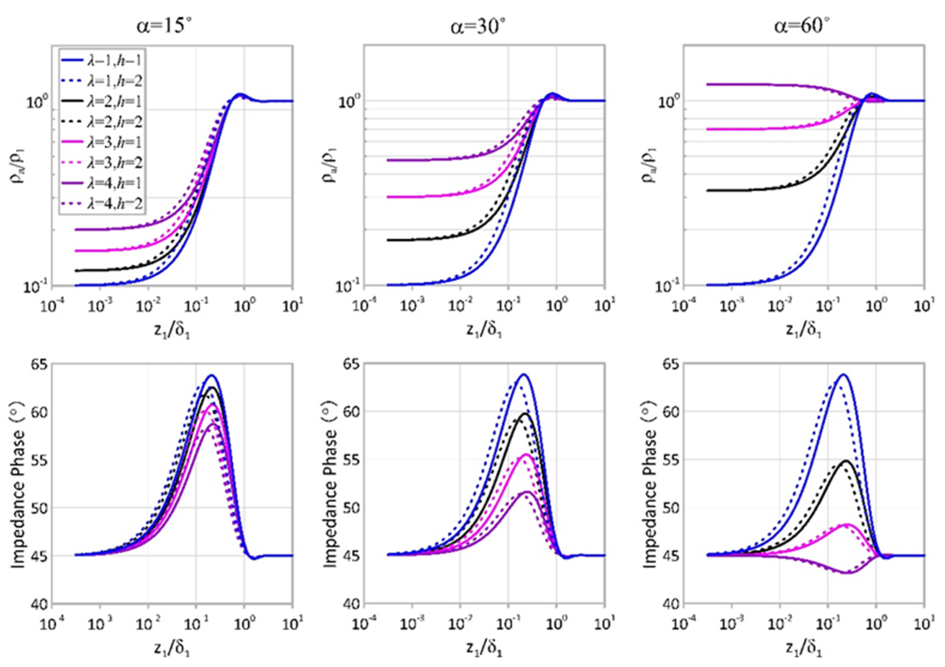
4. Dependence of the Apparent Resistivity and Impedance Phase on the Model Parameters

In this part of the study, the dependence of the apparent resistivity and impedance phase on the model parameters (dip angle, anisotropic coefficient and layer thickness) was investigated.

For the simplicity of analysis, the conductivity in the top layer and the longitudinal conductivity in the bottom layer were kept unchanged (${\sigma }_1={0.01 }_{}\mathrm{S}/\mathrm{m}$, ${\sigma }_{l3}={0.1 }_{}\mathrm{S}/\mathrm{m}$) in the following calculation, and then we considered the variations in MT responses with other parameters (dip angle $\alpha$, anisotropic coefficient $\lambda$ and normalized thickness $h$). The normalized thickness was defined as $h=\left[\left(z_2-z_1\right)-z_1\right]/z_1$, and the anisotropic coefficient $\lambda$ was defined in Section 2.1.

To provide an integrated insight into the influence of various parameters on MT responses, three values were chosen for the anisotropic dip angles ($\alpha =15°, 30°, \mathrm{and} 60°$), and four values were assigned for the anisotropic coefficient ($\lambda =1, 2, 3, \mathrm{and} 4)$ in the case of two different normalized thicknesses of the transitional layer ($h=1, 2)$ in the calculation. The results are shown in Figure 4. For the convenience of plotting, dimensionless quantities were adopted. That is, the apparent resistivity normalized by the resistivity of the first layer and the impedance phases were plotted against the normalized skin depth $z_1/{\delta }_1$, where ${\delta }_1$ represents the skin depth of the incident EM wave with a given frequency in a half-space with the conductivity value of ${\sigma }_1$. Additionally, it is worth noting that the impedance phase was transformed into the first quadrant.

For given anisotropic coefficients and dip angles, it is clear from the top panels in Figure 4 that as the value of $h$ is increased from 1 to 2, the values of the normalized apparent resistivity increased correspondingly for intermediate values of $z_1/{\delta }_1\left(0.1-1.0\right)$, except for the case of $\alpha =60°$ and $\lambda =4$, while no difference may be seen for very large (>1.0) or very small values (<0.01) of $z_1/{\delta }_1$. The bottom panels in Figure 4 show that the impedance phase first increased with an increasing $h$ until it reached the peak value and then decreased with $h$ (except for the case of $\alpha =60°$ and $\lambda =4$). It is also obvious that the extremum value of the impedance phase decreased as $h$ increased. A possible explanation for this phenomenon is that due to the increase in the thickness of the middle layer, more EM energy was attenuated in this layer; thus, the energy reflected from the lower boundary decreased, and a less destructive interference with the incident wave was created in this case.

For a given anisotropic dip angle, as the value of the anisotropic coefficient ($\lambda$) increases, the normalized apparent resistivity and impedance phase change proportionally. These most significant changes appeared in the normalized apparent resistivity for smaller values of $z_1/{\delta }_1$ (<1) and in the impedance phase for intermediate values of $z_1/{\delta }_1$ (0.01–1). Additionally, the normalized apparent resistivity and impedance phase are independent of the anisotropic dip angles if the basement layer becomes isotropic (the blue solid or dashed curves marked by $\lambda =1$ in the legend). The increase in the anisotropic coefficient ($\lambda$) implies a decrease (or increase) in the conductivity (resistivity) in the transverse direction, and the EM energy reflected from the third layer increases and may create more constructive interference with the incident EM wave.

For a given anisotropic coefficient (except for $\lambda =1$), the normalized apparent resistivity increases as $h$ increases; however, the impedance phase shows the opposite characteristic.

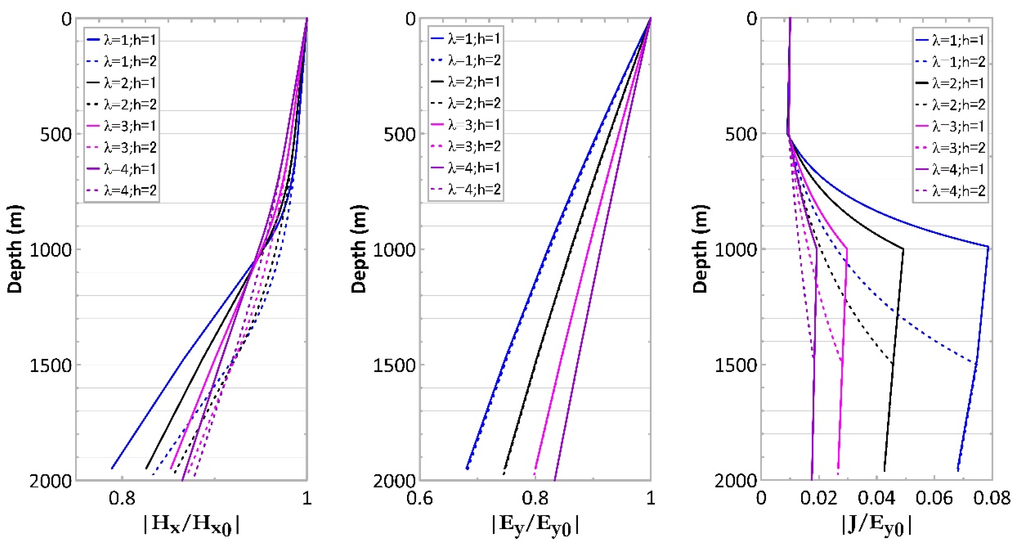
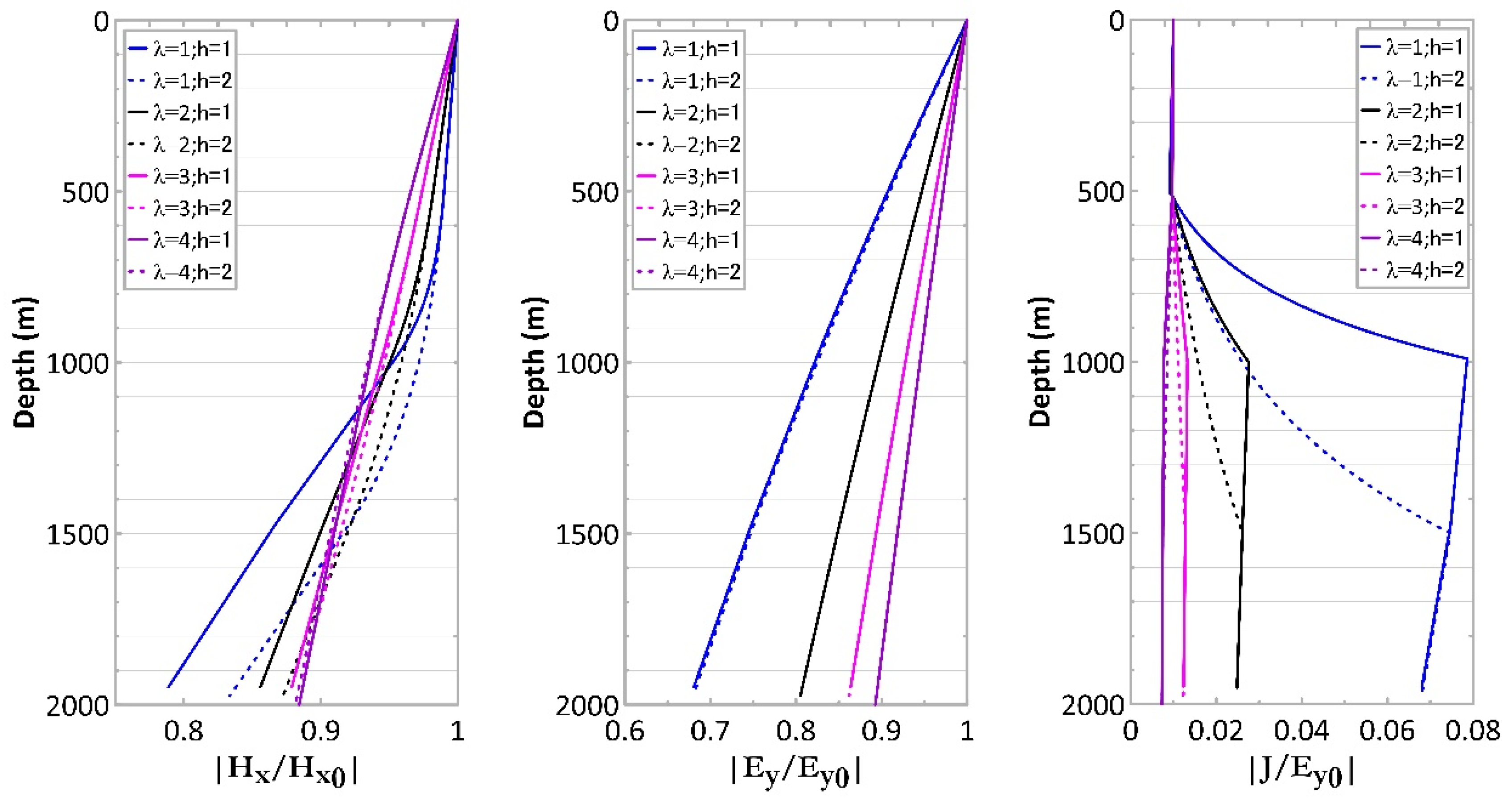
5. Discussion: Variations in the EM Fields with Model Parameters

In the previous section, the dependence of the apparent resistivity and impedance phase on the model parameters were investigated. In this section, we discuss how the intensity of the anisotropy and dip angle affect the current and EM fields in each layer. The models considered here are the same as those used in the previous section. The thickness of the top layer is fixed at 500 m, while the thickness of the transitional layer is assigned as 500 m and 1000 m, which correspond to $h=1$ and $h=2$ in the previous section. The variations in the EM fields and current density with depth at a period of 10 s are presented as an example. Because the lower boundaries of the transitional layer in the two cases are located at depths of 1000 m and 1500 m, only the results at depths ranging from 0 to 2000 m are shown (Figure 5, Figure 6 and Figure 7). The variations in the EM fields and current density with depth for the anisotropic models with dip angles of 15°, 30° and 60° are presented in Figure 5, Figure 6 and Figure 7. To show the attenuation of the EM fields with depth, the EM fields are normalized by the values at the surface of the model. Additionally, in order to more clearly show the influences of the transitional and anisotropic layers rather than the top layer on the current density, the current density was normalized by the electric fields at the surface of the model.

The attenuations of the magnetic fields are presented in the left-hand panels in Figure 5, Figure 6 and Figure 7, and the attenuation characteristics are different in different layers. The attenuations are nearly linear with the depth in the first layer, and the differences in the attenuations for different models are indistinguishable and may be neglected when the dip angle is 15° (left-hand panel in Figure 5), and the differences become distinguishable as the angle increases (left-hand panels in Figure 6 and Figure 7). At the approximate depths of the lower boundary of the transitional layer (1000 and 1500 m), the decay curves for different models merge when the dip angle is 15° (left panel in Figure 5) and 30° (left panel in Figure 6). The attenuation of the magnetic fields is strongly affected by the middle layer’s thickness.

For the attenuation of the electric field shown in the middle panels in Figure 5, Figure 6 and Figure 7, it is clear that the electric field is always continuous across layers with different conductivities, and the attenuation is approximately linear with depth at 0–2000 m. With the increase in the values of the dip angle in the model, the attenuation of the electric fields decreases, except when the basement layer is isotropic (blue lines). The effect of the middle layer’s thickness on the electric fields is negligible.

A comparison of the attenuation of the magnetic fields in the left-hand panels and the electric fields in the middle panels in Figure 5, Figure 6 and Figure 7 also shows that the influence of the transitional and anisotropic layers on the magnetic fields is more significant than that on the electric fields.

According to Ohm’s law ($J=\mathsf{\sigma }E$), the current should diffuse at the same rate as the electric field in each layer. However, the magnitude of the current depends on the value of the conductivity of the medium, and therefore, in general, different conductivities always cause different currents at the interfaces between layers. This phenomenon is evident in the right-hand panels in Figure 5, Figure 6 and Figure 7. Of note, the diffusion of the current is almost the same as that in the first layer for these cases.

6. Conclusions

In this work, the EM fields of a 1D stratified model containing a middle transition layer of exponentially varying conductivity with depth were explicitly solved. The conductivity in the transition layer may increase or decrease with depth depending on the conductivity value in the top and bottom layers. The electric and magnetic fields in the transitional layer are written in the form of modified Bessel functions.

The dependence of the apparent resistivity and impedance phase on the dip angles, anisotropic coefficient and normalized thickness were investigated in detail. The influence of the intensity of anisotropy and dip angle on the current and EM fields was also examined. The attenuation of the electric fields is almost linear with depth, while the attenuation of the magnetic field is nonlinear. The variation of the magnetic fields with depth is strongly affected by the middle layer’s thickness and the anisotropic coefficient. The variation in the current density with depth in the transitional layer is similar to the feature of the conductivity. The interfaces between layers are clearly seen from the current density profile.

The obtained results may be useful for studying and understanding the attenuation of the EM fields in the Earth. The simple models may also be convenient for testing computational programs.

References

1. Cagniard, L. Basic Theory of the MT methods of Geophysical Propecting. Geophysics 1953, 18, 605–635. [Google Scholar] [CrossRef]
2. Tikhonov, A.N. The determination of the electrical properties of the deep layers of the earth’s crust. Dokl. Acad. Nauk. SSR 1950, 73, 295–297. (In Russian) [Google Scholar]
3. Tikhonov, A.N. On determining electrical characteristics of the deep layers of the earth’s crust. In Magnetotelluric Methods; Vozoff, K., Ed.; Society of Exploration Geophysicists: Tulsa, Oklahoma, 1986; pp. 2–3. [Google Scholar]
4. Wannamaker, P.E.; Stodt, J.A.; Rijo, L. PW2D—Finite Element Program for Solution of Magnetotelluric Responses of Two-Dimensional Earth Resistivity Structure; User Documentation; Earth Sciences Lab-158; Utah University Research Institute: Salt Lake City, UT, USA, 1985. [Google Scholar]
5. Wannamaker, P.E.; Stodt, J.A.; Rijo, L. A stable finite-element solution for two-dimensional magnetotelluric modeling. Geophys. J. R. Astron. Soc. 1987, 88, 277–296. [Google Scholar] [CrossRef] [Green Version]
6. Mackie, R.L.; Madden, T.R.; Wannamaker, P.E. Three-dimensional magnetotelluric modeling using difference equations-Theory and comparisons to integral equation solutions. Geophysics 1993, 58, 215–226. [Google Scholar] [CrossRef] [Green Version]
7. Pek, J.; Verner, T. Finite-difference modelling of magnetotelluric fields in two-dimensional anisotropic media. Geophys. J. Int. 1997, 128, 505–521. [Google Scholar] [CrossRef]
8. Li, Y.G. A finite-element algorithm for electromagnetic induction in two-dimensional anisotropic conductivity structures. Geophys. J. Int. 2002, 148, 389–401. [Google Scholar] [CrossRef] [Green Version]
9. Yang, C. MT numerical simulation of symmetrically 2D anisotropic media based on the finite element method. Northwest. Seismol. J. 1997, 19, 27–33. (In Chinese) [Google Scholar]
10. Newman, G.A.; Alumbaugh, D.L. Three-dimensional magnetotelluric inversion using non-linear conjugate gradients. Geophys. J. Int. 2000, 140, 410–424. [Google Scholar] [CrossRef] [Green Version]
11. Avdeev, D.; Avdeeva, A. 3D magnetotelluric inversion using a limited-memory quasi-Newton optimization. Geophysics 2009, 74, F45–F57. [Google Scholar] [CrossRef] [Green Version]
12. Siripunvaraporn, W.; Egbert, G. WSINV3DMT: Vertical magnetic field transfer function inversion and parallel implementation. Phys. Earth Planet. Inter. 2009, 173, 317–329. [Google Scholar] [CrossRef]
13. Egbert, G.D.; Kelbert, A. Computational recipes for electromagnetic inverse problems. Geophys. J. Int. 2012, 189, 251–267. [Google Scholar] [CrossRef] [Green Version]
14. Čuma, M.; Gribenko, A.; Zhdanov, M.S. Inversion of magnetotelluric data using integral equation approach with variable sensitivity domain: Application to EarthScope MT data. Phys. Earth Planet. Inter. 2017, 270, 113–127. [Google Scholar] [CrossRef]
15. Singh, A.; Dehiya, R.; Gupta, P.K.; Israil, M. A MATLAB based 3D modeling and inversion code for MT data. Comput. Geosci. 2017, 104, 1–11. [Google Scholar] [CrossRef]
16. Grayver, A.V. Parallel three-dimensional magnetotelluric inversion using adaptive finite-element method. Part I: Theory and synthetic study. Geophys. J. Int. 2015, 202, 584–603. [Google Scholar] [CrossRef] [Green Version]
17. Kordy, M.; Wannamaker, P.; Maris, V.; Cherkaev, E.; Hill, G. 3-D magnetotelluric inversion including topography using deformed hexahedral edge finite elements and direct solvers parallelized on SMP computers–Part I: Forward problem and parameter Jacobians. Geophys. J. Int. 2016, 204, 74–93. [Google Scholar] [CrossRef]
18. Kruglyakov, M.; Kuvshinov, A. 3-D inversion of MT impedances and inter-site tensors, individually and jointly. New lessons learnt. Earth Planets Space 2019, 71, 1–9. [Google Scholar] [CrossRef] [Green Version]
19. Kruglyakov, M.; Geraskin, A.; Kuvshinov, A. Novel accurate and scalable 3-D MT forward solver based on a contracting integral equation method. Comput. Geosci. 2016, 96, 208–217. [Google Scholar] [CrossRef] [Green Version]
20. Seama, N.; Baba, K.; Utada, H.; Toh, H.; Tada, N.; Ichiki, M.; Matsuno, T. 1-D electrical conductivity structure beneath the Philippine Sea: Results from an ocean bottom magnetotelluric survey. Phys. Earth Planet. Inter. 2007, 162, 2–12. [Google Scholar] [CrossRef]
21. Ádám, A.; Novák, A.; Szarka, L. Basement depths of 3D basins, estimated from 1D magnetotelluric inversion. Acta Geod. Geophys. Hung. 2007, 42, 59–67. [Google Scholar] [CrossRef]
22. Oskooi, B. 1D interpretation of the Magnetotelluric data from Travale Geothermal Field in Italy. J. Earth Space Phys. 2006, 32, 1–16. [Google Scholar]
23. Ariani, E.; Srigutomo, W. 1D and 2D occam’s inversion of magnetotelluric data applied in Volcano-Geothermal area in Central Java, Indonesia. J. Phys. Conf. Ser. 2016, 739, 012039. [Google Scholar] [CrossRef]
24. Lichoro, C.M.; Árnason, K.; Cumming, W. Resistivity imaging of geothermal resources in northern Kenya rift by joint 1D inversion of MT and TEM data. Geothermics 2017, 68, 20–32. [Google Scholar] [CrossRef]
25. Marsenić, A. Understanding 1D magnetotelluric apparent resistivity and phase. J. Electromagn. Waves Appl. 2020, 34, 246–258. [Google Scholar] [CrossRef]
26. Reddy, I.K.; Rankin, D. Magnetotelluric effect of dipping anisotropies. Geophys. Prospect. 1971, 19, 84–97. [Google Scholar] [CrossRef]
27. Loewenth, D.; Landisma, M. Theory for magnetotelluric observations on surface of a layered anisotropic half space. Geophys. J. R. Astron. Soc. 1973, 35, 195–214. [Google Scholar] [CrossRef]
28. Shoham, Y.; Loewenthal, D. Magnetotelluric impedance tensor computational for an anisotropic 1-Dimensional layered media. Geophysics 1975, 40, 155. [Google Scholar]
29. Kaufman, A.A.; Keller, G.V. The Magnetotelluric Sounding Method. Methods in Geochemistry and Geophysics; Elsevier Scientific: Amsterdam, The Netherlands, 1981; Volume 15, p. 596. [Google Scholar]
30. Yungul, S.H. Magnetotelluric sounding three-layer interpretation curves. Geophysics 1961, 26, 465–473. [Google Scholar] [CrossRef]
31. Patella, D. Interpretation of magnetotelluric resistivity and phase soundings over horizontal layers. Geophysics 1976, 41, 96–105. [Google Scholar] [CrossRef]
32. Mallick, K. Magnetotelluric sounding on a layered earth with transitional boundary. Geophys. Prospect. 1970, 18, 738–757. [Google Scholar] [CrossRef]
33. Srivastav, J.; Niwas, S. Magnetotellurics sounding over models of continuously varying conductivity. Proc. Natl. Acad. Sci. USA India Sect. A 1976, 42, 320–327. [Google Scholar]
34. Kao, D.; Rankin, D. Magnetotelluric response on inhomogeneous layered earth. Geophysics 1980, 45, 1793–1802. [Google Scholar] [CrossRef]
35. Kao, D. Magnetotelluric Response on Vertically Inhomogeneous Earth. J. Geophys. Res. 1981, 86, 3027–3038. [Google Scholar] [CrossRef]
36. Kao, D. Magnetotelluric response on vertically inhomogeneous earth having conductivity varying exponentially with depth. Geophysics 1982, 47, 89–99. [Google Scholar] [CrossRef]
37. Banerjee, B.; Sengupta, B.J.; Pal, B.P. Apparent resistivity of a multilayered earth with a layer having exponential variation of conductivity. Geophys. Prospect. 1980, 28, 430–452. [Google Scholar] [CrossRef]
38. Peterson, F.L.; Lao, C. Electric well logging of Hawaiian basaltic aquifers. Groundwater 1970, 8, 11–18. [Google Scholar] [CrossRef]
39. Spichak, V.V.; Zakharova, O.K. Porosity estimation at depths below the borehole bottom from resistivity logs and electromagnetic resistivity. Near Surf. Geophys. 2016, 14, 299–306. [Google Scholar] [CrossRef]
40. Asfahani, J. Porosity and hydraulic conductivity estimation of the basaltic aquifer in Southern Syria by using nuclear and electrical well logging techniques. Acta Geophys. 2017, 65, 765–775. [Google Scholar] [CrossRef]
41. Berdichevsky, M.; Dmitriyev, V.; Mershchikova, N. Investigation of gradient media in deep electromagnetic sounding. 1ZV Akad. Nauk SSSR Series Fiz. Zemli 1974, 10, 61–72. [Google Scholar]
42. Kim, H.-S.; Lee, K. Response of a multilayered earth with layers having exponentially varying resistivities. Geophysics 1996, 61, 180–191. [Google Scholar] [CrossRef]
43. Pal, B.P. Magnetotelluric response on a layered earth with non-monotonic resistivity distribution. In Deep Electromagnetic Exploration; Narosa Publishing House: New Delhi, India, 1998; pp. 425–431. [Google Scholar]
44. Berdichevsky, M.N.; Dmitriev, V.I. Magnetotellurics in the Context of the Theory of Ill-Posed Problems; Society of Exploration Geophysicists: Tulsa, OK, USA, 2002. [Google Scholar]
45. Yoshio, K.; Takehiko, K. On the Phase Difference of Earth Current Induced by the Changes of the Earth’s Magnetic Field. Sci. Rep. Tohoku Univ. 1950, 2, 138–141. [Google Scholar]
46. Qin, L.; Yang, C. Magnetotelluric Soundings on a Stratified Earth with Two Transitional Layers. Pure Appl. Geophys. 2020, 177, 5263–5274. [Google Scholar] [CrossRef]
47. Negi, J.G.; Saraf, P.D. Inductive sounding of a stratified earth with transition layer resting on dipping anisotropic beds. Geophys. Prospect. 1973, 21, 635–647. [Google Scholar] [CrossRef]
48. Kovacikova, S.; Pek, J. Generalized Riccati equations for 1-D magnetotelluric impedances over anisotropic conductors Part I: Plane wave field model. Earth Planets Space 2002, 54, 473–482. [Google Scholar] [CrossRef] [Green Version]
49. Qin, L.; Yang, C.; Ding, W. Magnetotelluric responses of a vertical inhomogeneous and anisotropic resistivity structure with a transitional layer. Acta Geod. Geophys. 2022, 57, 157–176. [Google Scholar] [CrossRef]
50. Chlamtac, M.; Abramovici, F. The electromagnetic fields of a horizontal dipole over a vertically inhomogeneous and anisotropic earth. Geophysics 1981, 46, 904–915. [Google Scholar] [CrossRef]
51. Zima, L. The Interpretation of Resistivity Sounding over Weathered Rocks. Geophys. Trans. 1987, 32, 319–332. [Google Scholar]
52. Sinha, A.K. The magnetotelluric effect in an inhomogeneous and anisotropic earth. Geoexploration 1969, 7, 9–28. [Google Scholar] [CrossRef]
53. Cavaliere, T.; Jones, A.G. On the identification of a transition zone in electrical conductivity between the lithosphere and asthenosphere: A plea for more precise phase data. J. Geophys. 1984, 55, 23–30. [Google Scholar]
54. Simpson, F.; Bahr, K. Practical Magnetotellurics; Cambridge University Press: Cambridge, UK, 2005. [Google Scholar]
55. Chave, A.D.; Jones, A.G. The Magnetotelluric Method: Theory and Practice; Cambridge University Press: Cambridge, UK, 2012. [Google Scholar]
56. Boas, M.L. Mathematical Methods in the Physical Sciences; John Wiley & Sons: Hoboken, NJ, USA, 2006. [Google Scholar]
57. Persidis, S. Mathematical Handbook; ESPI Publishing: Athens, Greece, 2007. [Google Scholar]
58. Negi, J.; Saraf, P. Impedance of a Plane Electromagnetic Wave at the Surface of a Layered Conducting Earth with Dipping Anisotropy. Geophys. Prospect. 1972, 20, 785–799. [Google Scholar] [CrossRef]
59. Pek, J.; Santos, F.A.M. Magnetotelluric impedances and parametric sensitivities for 1-D anisotropic layered media. Comput. Geosci. 2002, 28, 939–950. [Google Scholar] [CrossRef]
Figure 1. A 1D layered anisotropic model containing three layers. The black axes are for the coordinate system. The top layer is an isotropic layer of fixed conductivity σ 1 . The middle layer is a transitional layer of conductivity that varies exponentially with depth, represented by σ 2 ( z ) . The bottom layer is a dipping anisotropic bed of conductivities σ l 3 and σ t 3 in the longitudinal and transverse directions, respectively, in the o-xyz coordinate system. The variation in conductivity with depth in the top and middle layers are represented by the grey line and the curve, respectively, and the anisotropic conductivities in the bottom layer are marked by grey arrows. The dipping direction of the bottom bed makes an angle α with the horizontal interface.
Minerals 12 00915 g001
Figure 2. The 1D layered model contains a layer of exponentially varying conductivity (black solid curve) and a stair-step model with steps of 200 m (magenta solid curve), 100 m (blue solid curve) and 20 m (green solid curve). The exponentially varying conductivity model is represented by the “Exponential model” in the legend, and the stair-step model with a step of 200 m is marked as “Step = 200 m” (and similarly for the other stair-step models). Please note that the bottom layer (the anisotropic layer) is not shown in the figure.
Minerals 12 00915 g002
Figure 3. Comparison of the MT soundings given by the algorithm presented in this work for the exponential model denoted by the black solid line shown in Figure 2 and those obtained using the Pek1DAniCode for the stair-step models shown by magenta, blue and green dashed lines in Figure 2. (a) Apparent resistivity. (b) Impedance phase. (c) Relative error (RE) of the apparent resistivity. (d) Phase difference (PD). The results calculated using the method in this study are as by “Analytic solution” in the legend, and the results for the stair-step model with a step of 200 m are marked as “Step = 200 m” (and similarly for the other stair-step models). See the text for details.
Minerals 12 00915 g003
Figure 4. The normalized apparent resistivity (top panels) and impedance phase (bottom panels) at the surface of the vertical inhomogeneous and anisotropic Earth with various model parameters. ρ 1   is the resistivity of the first layer and the inverse of σ 1 ; δ 1 = 2 / ω μ σ 1 is the skin depth of the incident EM wave with a given frequency and the conductivity in the top layer. The curves presented in the left, middle and right columns correspond to three different dip angles. In each panel, the results for different anisotropic coefficients are marked by curves in different colours, while those for the normalized thicknesses of 1 and 2 are marked by solid and dashed lines, respectively.
Minerals 12 00915 g004
Figure 5. The variation in the amplitude of the normalized magnetic field (left panel), electric field (middle panel) and current density (right panel) with depths ranging from 0 to 2000 m for the anisotropic model with a dip angle of 15° in the bottom layer at a period of 10 s.
Minerals 12 00915 g005
Figure 6. Similar to the case shown in Figure 5 except that the anisotropic dip angle is 30° in the model.
Minerals 12 00915 g006
Figure 7. Similar to the case shown in Figure 5 except that the anisotropic dip angle is 60° in the model.
Minerals 12 00915 g007
Publisher’s Note: MDPI stays neutral with regard to jurisdictional claims in published maps and institutional affiliations.