Reservoir Characterization of a Tight Gas Field Using New Modified Type Curves for Production Data Analysis—A Case Study from Ordos Basin

Abstract

Using data from 56 tight gas wells from the study field (Y field) in the Ordos basin of China, this paper presents performance-based reservoir characterization of the study field from production data and geophysical data. Post-fracturing evaluation is realized by applying our new modified production decline type curves for fractured wells. Compared to traditional type curves, our newly proposed modified dimensionless type curves help identify field data diagnostics for various flow regimes of fractured wells and also facilitate the curve matching process with real data to obtain fruitful and crucial reservoir and fractured well information, including key parameters such as reservoir flowing capacity (kh), well productivity, fracture length, drainage area and original gas in place. This paper intends to promote the extensive application of this new technique. With the support of the reservoir information provided by production decline analysis using our modified type curves, the commercial flow units are delineated in terms of interrelated porosity-permeability of sandstone based on pore throat aperture crossplotting and corresponding flow unit productivity. Furthermore, two crossplots of well logging interpreted porosity versus resistivity are constructed, suggesting their good correlated relationships with relative flow unit productivity and initial gas abundance in place, respectively. The two crossplots enable qualitative evaluation of formation penetrated by well, which makes them very useful and practical as wireline logging is basically available for every well. The well production routine is also analyzed systematically by considering a well’s inflow performance, tubing performance and minimal liquid-carrying gas flow rate to investigate if a gas well is producing at optimal conditions or if a measure should be taken to improve the well’s production. Through analysis of the Y field, this study introduces an integrated workflow with the support of the new modified type curves to effectively help understand the reservoir characteristics and the flow behaviors of the tight gas field. The key takeaway from this study is that the new modified dimensionless production decline curves in terms of $q_{DM} vs. t_{DM}$ can be applied in field practice to achieve a systematically comparable understanding of the performance of MHFHWs globally.

1. Introduction

Located in the eastern Ordos basin of China, the Y field spans as large as 107.1 km² and is estimated to have a gas reserve of 1.08 × 10¹⁰ m³. The formation (Shihezi), consisting of eight pay beds (He1 to He8), was deposited under a braided delta system and the thickness of the pay beds ranges from 1.5 m to 12.5 m. The characteristics of core samples show that porosity ranges from 8% to 14%, air permeability from 0.2 to 3.0 mD, and gas saturation from 40% to 80%. The production history of the Y field is provided in Figure 1. The first well was initiated into production in January 2016 and the second well was put into production in May 2017. From then on, more and more wells were constantly drilled and completed for production. The peak gas rate of the field reached 72 × 10⁴ m³/d in October 2019 with 34 wells in production. In general, from April 2019, the gas rate started to show an obvious decline and only drilling more wells could compensate for the declining trend. After the peak rate, however, even though more new wells were completed to increase production, the total gas rate could not bounce back. Currently, 56 wells are in production in the field with a daily gas rate fluctuating around 50 × 10⁴ m³/d. Of all of the wells, 45 are hydraulically fractured and 11 are not fractured. This is the tough reality that the industry has to face in tight gas field exploitation; it is subject to rapid field rate decline. To increase economic gains and enhance ultimate recovery, with years of production data and experiences, a systematical study-based production dynamics analysis to improve the understanding of the formations and their flow characteristics is necessary and a suite of techniques for post-fracturing production data analysis needs to be established.

Zhao et al. [1] innovatively proposed modified production decline type curves for fractured wells. The post-fracturing production data of the Y field presented in this paper are mainly analyzed by the modified type curves with an extensive application, and detailed application procedures are also presented. Geophysical and well logging data are also used to support reservoir characterization of the Y field under study. To the authors’ knowledge, the proposed type curves are not currently available in any commercial software for rate-transient analysis or any published literature. Reparameterizing the production decline type curves using reservoir-well system parameters allows a systematical analysis of transient rate behaviors of fractured wells. This practice helps identify field data diagnostics effectively and facilitates the curve matching process as well as enhances confidence in analyzing the results. In addition, the key reservoir parameter, kh or well productivity (proportional to kh), evaluated by modified decline type curves is also applied in association with core sample analysis to delineate sandstone commercial flow units, in association with well logging facies to evaluate formation quality.

2. Methodologies and Applications

2.1. Post-Fracturing Evaluation

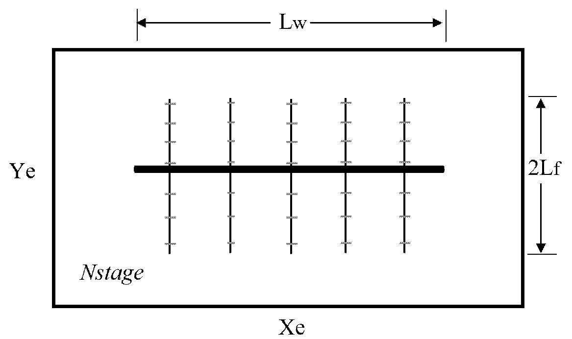
In this study, post-fracturing evaluation is performed to obtain reservoir flowing capacity, well productivity, drainage area, fracture length and original gas in place. The analytic modeling method for multistage hydraulically fractured horizontal well (MHFHW) [2,3] and the model-based modified production decline type curves proposed by Zhao et al. [1,2,3] are applied to achieve such objectives. The theoretical model of the MHFHW is schematically illustrated in Figure 2.

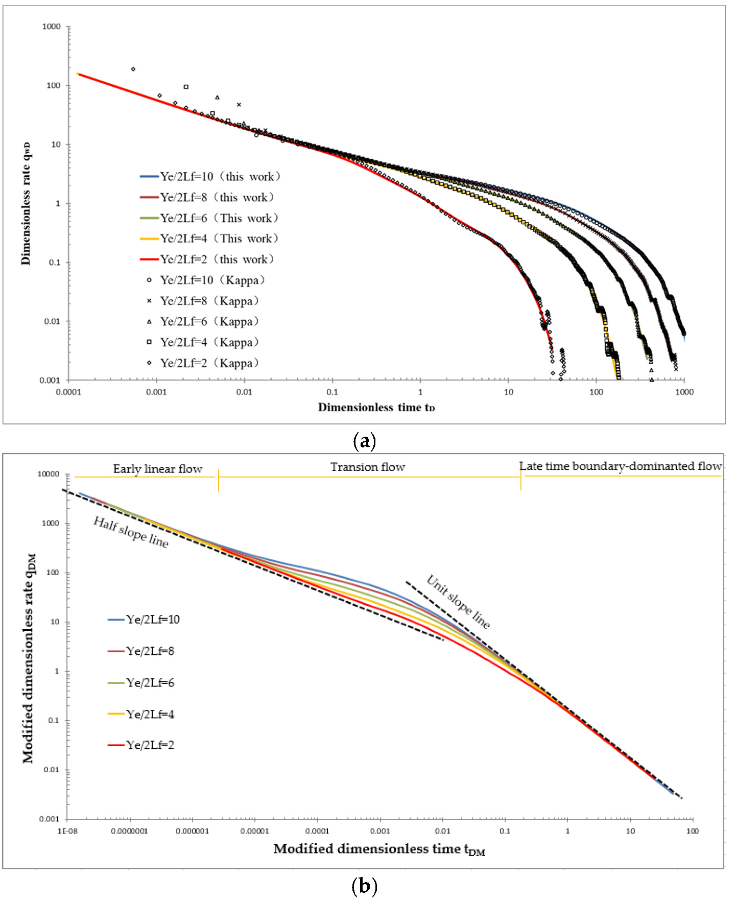
The analytical transient rate solutions of fractured horizontal well with parameters summarized in

Table 1. Basic parameters of the reservoir and well system for the theoretical case.

Porosity	0.2	Reservoir initial pressure (MPa)	34.01
Viscosity (cp)	1	Downhole flowing pressure (MPa)	13.61
Permeability (mD)	2	Compressibility (MPa−1)	0.00118
Thickness (m)	30.48	Formation volume factor	1
Fracture stage	5	Reservoir width (m)	900
Stage space (m)	90	Reservoir length (m)	300

under various reservoir length to fracture length ratios are presented in Figure 3a in dimensionless form along with solutions generated by commercial reservoir software Kappa [4] for comparison and validation. Dimensionless well rate is defined as

$$q_D=\frac{1.84q_{w}B\mu }{kh\left(p_i-p_{wf}\right)} ,$$

(1)

and dimensionless time is defined as

$$t_D=\frac{0.086kt}{\varnothing \mu c_t{L}_f^2} .$$

(2)

It can be seen in Figure 3a that the two sets of rate solutions, in general, are in good agreement, while solutions generated by Zhao’s model are more stable and consistent at early and late times, which sets a solid foundation for the establishment of modified decline type curves for MHFHW.

Zhao et al. [1] innovatively defined modified dimensionless rate and modified dimensionless time, in which reservoir-fracture geometries are uniquely integrated to attain unique ways for the presentation of the modified type curves that allow a systematically universal analysis of transient rate behaviors of MHFHW.

The modified dimensionless terms are defined by the following equations as

$$q_{DM}=\frac{q_{wD}·Scaler}{N_{stage}},$$

(3)

$$t_{DM}=\frac{t_{mbD}}{Scale{r}^2} ,$$

(4)

where “Scaler” is defined as

$$Scaler=\frac{X_e·Y_e}{L_f^2}\times \frac{1}{N_{stage}} .$$

(5)

The curves in terms of $q_D vs. t_D$, illustrated in Figure 3a, are converted using Equations (3)–(5) and are replotted in the form of $q_{DM} vs. t_{DM}$ in Figure 3b. Note that the $q_D vs. t_D$ datasets with the reservoir information are documented in Appendix A to provide the opportunity of reproducing the type curves if interested. One can observe the significant feature update of the curves, especially in terms of the shapes of the group of the new type curves. In more detail, all curves fall on the same stem during early linear flow with a 1/2 slope decline trend and also on the same stem at late boundary-dominated flow (BDF) with a unit slope decline trend. This provides a unique feature for the type curve matching process and is the most innovative contribution of the modified dimensionless type curves for MHFHW. The modified type curves help identify field data diagnostics for various flow regime changes of fractured wells and also facilitate the curve matching process with real data to obtain the key information of a reservoir-fracture system.

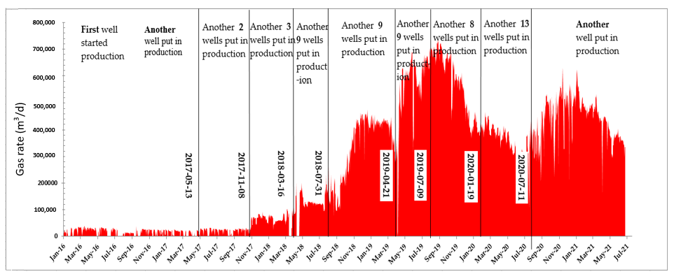
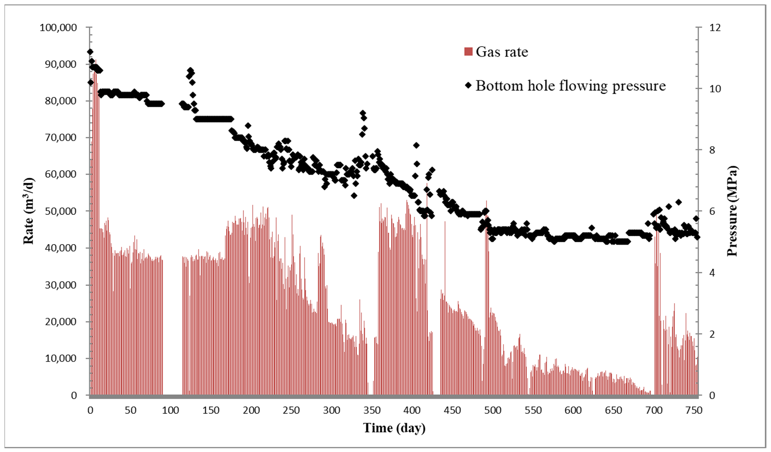
Taking a multistage fractured horizontal well, Y-9-1H, with five stages of transverse fracturing along horizontal wellbore trajectory as an example, Figure 4 shows its daily production rate and bottom hole flowing pressure and

Table 2. Basic parameters of the reservoir and the MHFHW Y-9-1H.

Temperature (°C)	42	Fracture stage(s)	5
Reservoir initial pressure (MPa)	12.44	Formation volume factor	0.0068
Porosity	0.127	Compressibility (MPa−1)	0.072
Thickness (m)	10.0	Viscosity (cp)	0.0163

summarizes the basic reservoir and well information. Post-fracturing evaluation by applying the modified decline type curves follows the procedures below:

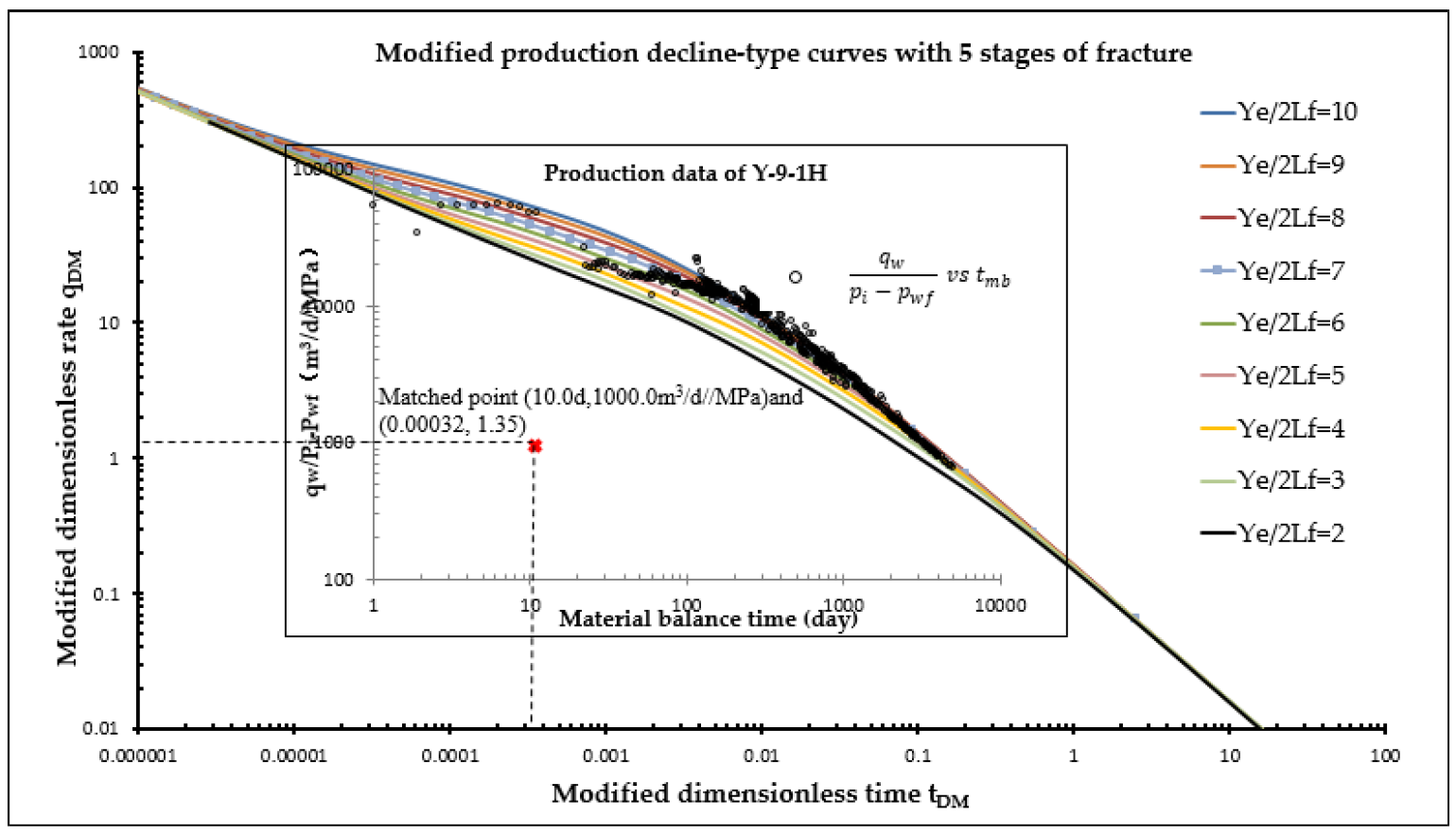
• Based on geophysical and geological information, simplify the reservoir boundary as rectangular shape and interpret reservoir width/length ratio as $X_e/Y_e=3/1$ for this case, and generate the modified type curves under various reservoir length and fracture length ratios.
• Plot gas well dynamic rate data as pressure drop normalized rate, $\frac{q_w}{p_i-p_{wf}} ,$ vs. material balance time, $t_{mb}$.
• Match well dynamic data plot $\frac{q_w}{p_i-p_{wf}}$ vs. $t_{mb}$ with type curves of $q_{DM} vs. t_{DM}$. In this case, as illustrated by Figure 5, well data achieves the best match with the type curve $Y_e/2L_f=7$ with$Scaler=\frac{X_e·Y_e}{L_f^2}\frac{1}{N_{stage}}=14\times 14\times 3\times \frac{1}{5}=117.6$, and coordinates of the matched point in respective plot are $\left(10.0 \mathrm{d},1000.0{ \mathrm{m}}^3/\mathrm{d}/\mathrm{MPa}\right)$ and $\left(0.00032, 1.35\right)$, respectively. It is speculated that the deviation of early production data away from the corresponding type curve is subject to other factors, such as production data quality, non-Darcy flow, near-wellbore heterogeneity, etc. Further research work is needed.
• Calculate the objective parameters.

Based on definitions of $q_{DM}$ and $q_{wD}$, the kh value is solved by

$$kh=1.84B\mu \frac{Scaler}{N_{stage}}{\left(\frac{\frac{q_w}{\Delta p}}{q_{DM}}\right)}_{MP}=1.84\times 0.0068\times 0.0163\times \frac{117.6}{5}\times \frac{1000.0}{1.35}=3.55 m·mD ,$$

(6)

and based on the definitions of $t_{DM}$ and $t_D$, the fracture half-length is solved by

$$L_f=\sqrt{\frac{0.086k}{\phi \mu c_t}{\left(\frac{t_{mb}}{t_{DM}}\right)}_{MP}}\frac{1}{Scaler}=\sqrt{\frac{0.086\times \frac{3.55}{10.0}}{0.127\times 0.0163\times 0.072}\times \frac{10}{0.00032}}\times \frac{1}{117.6}=21.4 m ,$$

(7)

and based on the definition of “Scaler”, the drainage area of the fractured well can be calculated by

$$X_e·Y_e=Scaler\times L_f^2\times N_{stage}=117.6\times {21.4}^2\times 5=269,280.4 m^2 ,$$

(8)

and original gas in place is given as

$$\mathrm{G}=\frac{X_e{Y}_{e}h\phi \left(1-S_{wc}\right)}{B}=\frac{269,280.4\times 10\times 0.127\times 0.85}{0.0068}=4.27\times {10}^7 m^3.$$

(9)

finally, well productivity is defined as

$$J=\frac{q_w}{\overline{p}-p_{wf}} .$$

(10)

As original gas in place was solved, average reservoir pressure can be easily obtained by gas reservoir material balance equation so that productivity, by Equation (10), of Y-9-1H is ultimately calculated as 2.35 m³/d/MPa.

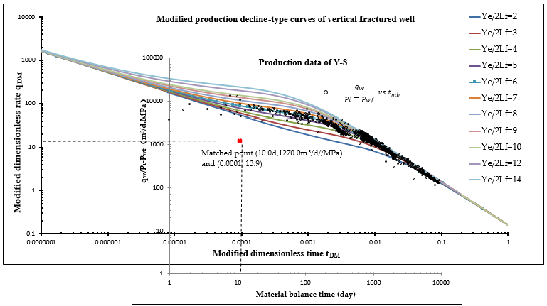
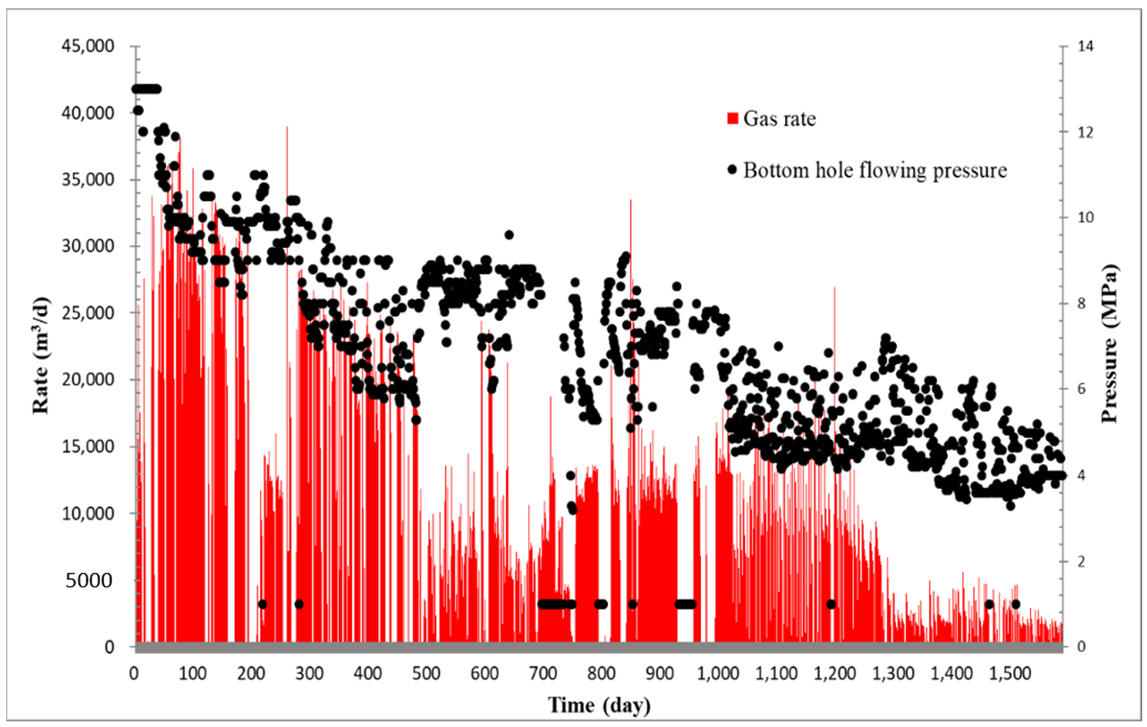
By applying a similar strategy and procedures, another case of a vertical fractured well, Y-8, is analyzed and presented. Figure 6 provides the daily production rate profile of Y-8 and with the associated well and reservoir parameters summarized in

Table 3. Basic parameters of the reservoir and well Y-8.

Temperature (°C)	45	Fracture stage	1
Reservoir initial pressure (MPa)	15.4	Formation volume factor	0.0056
Porosity	0.098	Compressibility (MPa−1)	0.067
Thickness (m)	6.1	Viscosity (cp)	0.0181

. For this case, the reservoir width/length ratio is interpreted as $X_e/Y_e=1/1$ with one stage of fracture assumed in the analytical model for modified dimensionless type curve generation. As shown in Figure 7, the well data achieves the best match with the type curve $Y_e/2L_f=6$ and the $Scaler=\frac{Y_e{Y}_e}{L_f^2}\frac{1}{N_{stage}}=12\times 12\times \frac{1}{1}=144$, and the coordinates of the matched point in the respective plot are $\left(10.0 \mathrm{d},1270.0{ \mathrm{m}}^3/\mathrm{d}/\mathrm{MPa}\right)$ and $\left(0.0001, 13.9\right)$, respectively. Similarly, kh value can be calculated by:

$$kh=1.84B\mu \frac{Scaler}{N_{stage}}{\left(\frac{\frac{q_w}{\Delta p}}{q_{DM}}\right)}_{MP}=1.84\times 0.0056\times 0.0181\times \frac{144}{1}\times \frac{1270.0}{13.5}=2.52 m·mD ,$$

(11)

and the fracture half-length is obtained by

$$L_f=\sqrt{\frac{0.086k}{\phi \mu c_t}{\left(\frac{t_{mb}}{t_{DM}}\right)}_{MP}}\frac{1}{Scaler}=\sqrt{\frac{0.086\times \frac{2.52}{6.1}}{0.098\times 0.0181\times 0.0522}\times \frac{10}{0.0001}}\times \frac{1}{144}=43.0 m ,$$

(12)

and the drainage area of Y-8 is solved by

$$X_e·Y_e=Scaler\times L_f^2\times N_{stage}=144\times {43.0}^2\times 1=266,256.0 m^2 ,$$

(13)

and original gas in place can be easily obtained by

$$\mathrm{G}=\frac{X_e{Y}_{e}h\phi \left(1-S_{wc}\right)}{B}=\frac{266,256.0\times 6.1\times 0.098\times 0.87}{0.0056}=2.47\times {10}^7 m^3.$$

(14)

Table 4. Post-fracturing evaluation of 13 wells by the modified type curves along with the results analyzed by the conventional Blasingame method for comparison.

Modified Type Curve Analysis						Blasingame Method Analysis
Well NO.	Drainage Area	Well Productivity	Fracture Length	Ye/2Lf	kh	Drainage Area	Well Productivity
	km2	104 m3/d/MPa	m	mD·m		km2	104 m3/d/MPa
1	0.270	2.35	43	7	3.55	0.240	2.08
2	0.267	0.88	86	6	2.53	0.293	0.96
3	0.052	0.58	46	5	1.22	0.054	0.60
4	0.223	0.40	118	4	0.73	0.244	0.44
5	0.022	0.24	30	5	0.75	0.023	0.25
6	0.097	0.49	52	6	1.90	0.110	0.56
7	0.111	0.36	67	5	1.30	0.178	0.58
8	0.441	3.39	110	6	3.04	0.443	3.41
9	0.328	0.57	115	5	1.47	0.362	0.63
10	0.406	2.05	106	6	5.70	0.470	2.37
11	0.095	0.72	39	7	1.19	0.106	0.81
12	0.059	0.31	61	4	1.06	0.041	0.22
13	0.095	1.19	62	5	0.74	0.096	1.20

summarizes the analyzing results of 13 wells with good production data quality by proposed modified decline type curves. In addition, well drainage area and well productivity analyzed by conventional Blasingame method [5,6] are also provided for comparison. The two sets of results show good agreement with each other, which demonstrates reliability of analyzing results offered in Table 4. However, conventional Blasingame method is designed only for late time analysis since the beginning of BDF for drainage area and well productivity. Fracture geometry and reservoir flowing capacity, which mainly depend on early linear flow period and transition period for evaluation, cannot be calculated by conventional Blasingame method. As displayed in Table 4, the proposed modified type curves for fractured well analysis provide fruitful and important systematic information on reservoirs and fractured wells.

2.2. Commercial Flow Unit

Winland of Amoco developed an empirical equation for identifying and defining flow units of hydrocarbon reservoirs from an interrelated series of porosity-permeability crossplots and from pore throat aperture radius (r₃₅) corresponding to mercury saturation at 35% from mercury injection pressure test [7]. 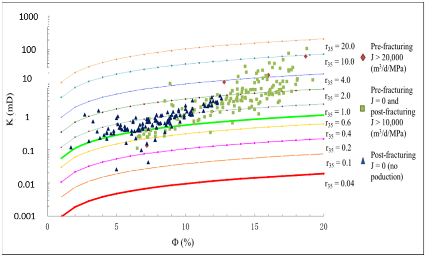On the basis of more than 2500 sandstone and carbonate samples originally used by Kwon and Pickett [8], Aguilera [7] developed the following equation to calculate the defined r₃₅

$$r_{35}=2.665{\left[k/\left(100\phi \right)\right]}^{0.45} .$$

(15)

With the application of Equation (15), a porosity-permeability crossplot under various r₃₅ values is established and presented in Figure 8, including data from 291 core samples of Y field. The red dots represent flow units with commercial productivity without fracturing stimulation, and the green dots represent flow units that are unable to achieve commercial productivity without fracturing operations but acquire productivity after fracturing, whereas the dark blue dots represent flow units that do not achieve commercial productivity even after fracturing. As illustrated in Figure 8, in general, a formation with r₃₅ greater than 4.0 does not require fracturing to produce, while one with r₃₅ greater than 1 and less than 4 needs fracturing to obtain reasonable productivity. However, a formation with r₃₅ less than 1 cannot possibly gain productivity even if fracturing stimulation is applied.

2.3. Identification of Water-Producing Reservoir

In order to minimize operation cost, water production rates of wells in Y field are not measured, which causes the problem that it is impossible to tell whether a reservoir is producing water or not from production data collected directly. As water plays a crucial role in tight gas reservoir production management and reservoir characterization, it is necessary to effectively identify water-production reservoirs by using various production and test data diagnostics.

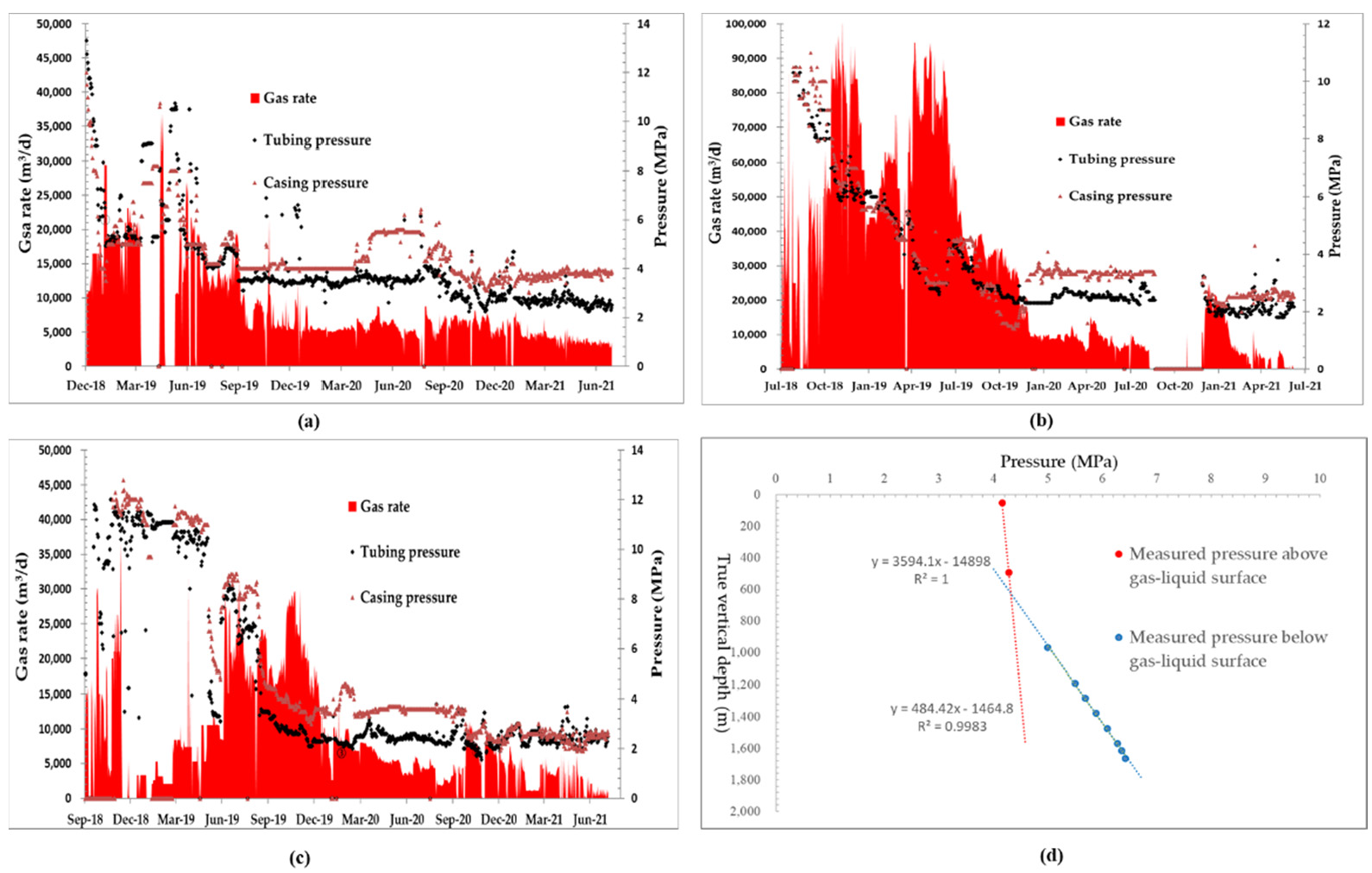
This study uses 4 empirical methods to identify if a gas well has water production. As illustrated in Figure 9 identifying 4 typical gas wells with water production due to water accumulation in tubing, they are: (a) gas rate increases along with tubing pressure rise, or it decreases along with tubing pressure; (b) tubing pressure drops below casing pressure; (c) gas rate experiences sharp drop from well shut-in to reopening; (d) flowing pressure test demonstrates fluid density change inside wellbore.

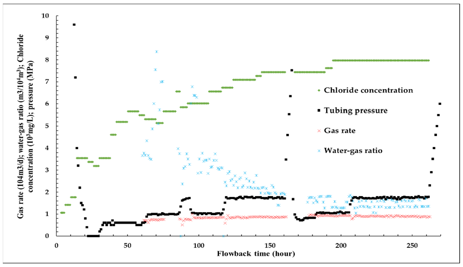
When a gas well is considered to have water production, its level of water production severity is characterized by the water–gas ratio (WGR) measured during flowback period when liquid rate, gas rate, tubing pressure and chloride concentration are stable. For example, as shown in Figure 10, after 120 h of flowback subsequent to fracturing treatment, data dynamics are stable and WGR approximately arrives at 1.5 m³/10⁴ m³.

2.4. Formation Quality Evaluation

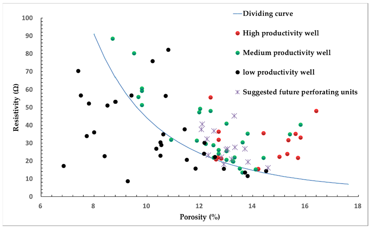
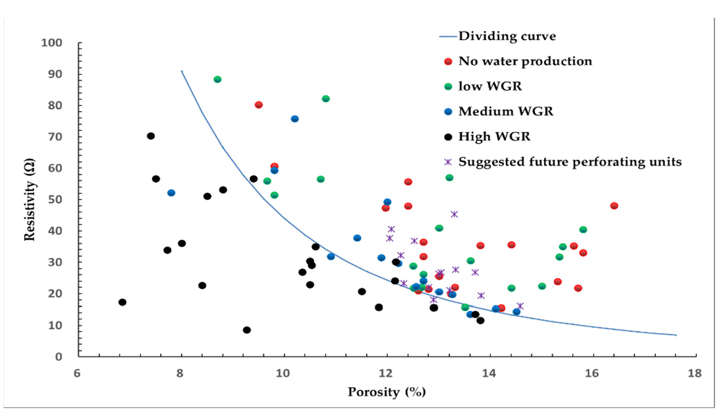
For the study field, gas productivity or in-place gas abundance (characterized by WGR) is found to correlate quite well with well logging information. Two useful plots for formation quality evaluation of the Y field are established in this study. Based on production data and well logs from 56 wells, Figure 11 and Figure 12 illustrate the well logging interpreted porosity and resistivity relationship corresponding to productivity index and WGR ratio of these wells, respectively. The blue curve of Figure 11 roughly separates low-productivity flow units from medium-to-high productivity flow units. The blue curve of Figure 12 roughly separates high water-bearing flow units from medium-to-low water-bearing flow units. The coupling of well logging information with geological and reservoir engineering data provides not only the two plots to help characterize the interrelated geophysical properties of the reservoir but also a powerful tool to support field development.

Based on well logging information of all 56 wells, including He1 to He8 other than He5, 16 sandstone flow units, which were initially ignored and not perforated to produce by all of the 12 wells, are found to have corresponding porosity-resistivity characteristics that fall in the medium-to-high productivity area in Figure 11 and also fall in the medium-to-low WGR area in Figure 12.

Table 5. Potentials of the 16 reservoir sands for the future perforation of the 12 wells.

Well No.	Current Producing Formation	Potential Formation to Perforate	Thickness	Porosity	Swc	Resistivity
			m	%	%	Ω
1	He7	He1	0.7	13.00	23.30	26.30
2	He7	He6	2.0	13.29	37.76	45.27
3	He7, He6, He4	He1	2.9	13.04	48.60	26.76
4	He6	He2	6.1	14.57	43.32	16.06
		He6	4.4	13.32	44.26	27.64
5	He6	He2	2.4	12.32	39.82	23.26
6	He6	He8	1.5	14.10	59.53	67.10
7	He4	He7	2.4	12.08	46.70	40.54
8	He7	He1	2.5	13.20	46.44	21.04
		He4	2.4	13.81	41.01	19.43
		He7	3.0	12.05	43.90	37.63
9	He6, He7	He3	2.6	12.53	43.26	36.86
10	He7, He6	He1	6.4	12.81	40.13	22.08
11	He7, He6	He4	4.1	12.90	52.65	18.10
12	He4	He2	3.2	13.70	54.46	26.74
		He2	3.5	12.27	58.32	32.24

summarizes related information of the 12 wells. Hence, the 12 wells have the opportunity to perforate such formation for production at a late stage to enhance ultimate recovery. Additionally, in order to seek productive layers that were previously ignored by the current production wells, Figure 6 and Figure 7 can be applied to qualitatively predict well performance when drilling and wireline logging are completed, or to decide whether a target layer switch for perforation is necessary.

Compared to general well logging techniques, e.g., applying Hingle and Pickett crosplotting for static information [9], Figure 11 and Figure 12 incorporated dynamic well productivity index and WGR information, therefore, the newly proposed innovative crossplotting technique and analysis strategy are valuable and practical.

2.5. Well Production Routine Analysis

Assuring that a gas well is producing at its optimal condition and taking measures to improve the well’s production are critical for the success of field development. A total of 3 curves, including inflow performance relationship (IPR), tubing performance relationship (TPR) and minimum gas rate performance relationship (MPR), are generated and used systematically to construct a diagnostic plot that helps find out the potential of raising gas rate, liquid loading problem in wellbore, or possible artificial lifting strategies to improve production. In this study, IPR is generated by well deliverability test, TPR is generated using commercial software Pipesim, and MPR is generated through the back-calculation method proposed by Lu et al. [10]. Turner [11] proposed a model to describe minimum gas flow rate for continuous liquid removal. Minimal gas velocity and minimal gas flow rate are mathematically formulated as

$$v_{cr}=X{\left[\frac{\sigma g({\rho }_l-{\rho }_g)}{{\rho }_g^2}\right]}^{0.25} ,$$

(16)

$$q_{cr}=2.5\times {10}^8\frac{A_{w}p{v}_{cr}}{ZT} .$$

(17)

The traditional approach requires a forward tubing flow model to calculate the value of the model coefficient, X in Equation (16), to generate MPR curve. Different forward models, however, result in different values of X ranging from 2.5 to 6.5, causing uncertainties. Lu et al. [9] proposed a simple and applicable method to solve this problem. By making use of flowing pressure gradient tests of producing gas wells, water accumulation status of a well that encounters liquid loading in wellbore can be readily recognized. 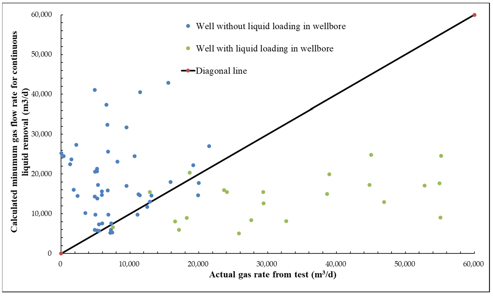Figure 13 shows the calculated minimum gas flow rate resulting with X = 2.8 versus the real gas well flow rate of the 35 wells in the study field. It is observable that a reasonably satisfying alignment near the 45° diagonal line can be achieved. Then, the MPR curve can be generated properly.

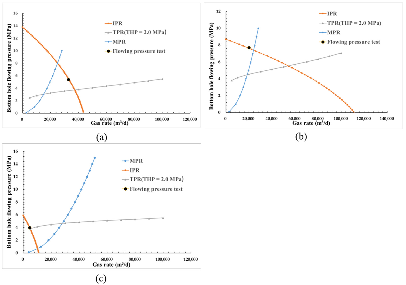
In the study, the 40 wells under study can be classified into 3 categories, based on the diagnostic plot composed of IPR, TPR and MPR curves, listed below:

Category 1: 

If the operational status on current IPR curve is above TPR curve but below MPR curve, as illustrated in Figure 14a, there exists no liquid loading in wellbore, therefore, either maintaining current producing routine or enlarging choke size can be recommended. There are 50% of the 40 wells belonging to Category 1.

Category 2: 

If the operational status on current IPR curve is above both TPR and MPR curves, as illustrated in Figure 14b, there exists liquid loading in wellbore, therefore, artificial lifting, or switching to tubing string with smaller size, is recommended. A total of 37.5% of the 40 wells belong to Category 2.

Category 3: 

If the operational status on current IPR curve is at the crossing point of IPR and TPR curves, and above MPR curve, as illustrated in Figure 14c, this suggests inadequate reservoir productivity and severe liquid loading in wellbore, therefore, the productivity of gas well is too low to be improved through tubing string design. A total of 12.5% of the 40 wells belong to Category 3.

3. Summary

Using the 56 tight gas wells’ production and geophysical data, we presented well performance-based tight gas reservoir characterization and production optimization for the field under study. The conclusions summarized from this study are:

• This work promotes the field application of the new modified dimensionless type curves proposed by Zhao et al. for production decline data analysis. Key information regarding reservoir and fractured wells, including reservoir flowing capacity (kh), productivity, drainage area, fracture length and original gas in place, can be obtained as well as the identification of complex flow regimes and the transitions of fractured wells. The unique diagnostic features of these newly proposed sets of type curves provide a powerful tool to evaluate post-fracturing production data because the production decline solutions during early time fracture linear flow and late time reservoir boundary dominant flow are uniquely placed at their own fixed positions in the new modified type curve setting. This unique feature not only established and promoted a systematical plotting and comparing strategy for MHFHWs globally, but also fundamentally offered the opportunity to further explore the effects of other hidden influencing factors on production decline, such as reservoir heterogeneity, enhancement of reservoir properties within SRV, and connected and disconnected natural fracture networks.
• Furthermore, the uniqueness of the type curve setting presented in the format of the new modified dimensionless terms allows a reliable and consistent engineering prediction of the MHFHW production performance under complicated real situations when production data are only partially available, such as the cases when only early time rate data, without late time boundary influence, are progressively collected during the early well production phase, or when only late time rate data are available because the production is normally reported monthly, likely missing the early time data. What makes such a reliable prediction possible is simply the fact that the rate responses of the early time fracture linear flow and the late time BDF are positioned at their fixed and unchanged locations.
• The integration of the results from the new modified production decline type curve analysis with those outcomes from the studies of core samples, well logging facies, and production optimization by using the diagnostic plots composed of IPR, TPR and MPR curves, facilitates the understanding of the reservoir characteristics and the flow behaviors of a tight gas field, thus helps enhance the ultimate gas recovery.

The key takeaway from this study is that the new modified dimensionless production decline curves in terms of $q_{DM} vs. t_{DM}$ can be applied in field practice to achieve a systematically comparable understanding of the performance of MHFHWs globally, with its unique feature that offers our reservoir engineers a new edge to deal with more complicated field cases.

References

1. Zhao, G.; Xiao, L.; Su, C.; Chen, Z.; Hu, K. Model-Based Type Curves and Their Applications for Horizontal Wells with Multi-Staged Hydraulic Fractures. Can. Energy Technol. Innov. (CETI) 2016, 2, 29–43. [Google Scholar]
2. Zhao, G. Reservoir Modeling Method. US Patent No. 8, 275, 593, 25 September 2012. [Google Scholar]
3. Zhao, G. A Simplified Engineering Model Integrated Stimulated Reservoir Volume (SRV) and Tight Formation Characterization with Multistage Fractured Horizontal Wells. In Proceedings of the SPE Canadian Unconventional Resources Conference, SPE-162806-MS. Calgary, AB, Canada, 30 October–1 November 2012. [Google Scholar]
4. Kappa Workstation Software of Dynamic Data Analysis; Version 5.20; Sophia-Antipolis: Valbonn, France.
5. Blasingame, T.A.; Lee, W.J. Variable-Rate Reservoir Limits Testing. In Proceedings of the Permian Basin Oil and Gas Recovery Conference, Midland, TX, USA, 13–14 March 1986; Society of Petroleum Engineers: Midland, TX, USA, 1986. [Google Scholar]
6. Blasingame, T.A.; Lee, W.J. The Variable-Rate Reservoir Limits Testing of Gas Wells. In Proceedings of the SPE Gas Technology Symposium, SPE-17708-MS. Dallas, TX, USA, 13–15 June 1988. [Google Scholar]
7. Aguilera, R. Incorporating Capillary Pressure, Pore Throat Aperture Radii, Height above Free-Water Table, and Winland R35 Values on Pickett Plots. AAPG Bull. 2002, 86, 605–624. [Google Scholar] [CrossRef]
8. Kwon, B.S.; Pickett, G.R. A New Pore Structure Model and Pore Structure Interrelationships. In Proceedings of the SPWLA 16th Annual Logging Symposium, SPWLA-1975-P. New Orleans, LA, USA, 4–7 June 1975. [Google Scholar]
9. Bassiouni, Z. Theory, Measurement, and Interpretation of Well Logs; SPE Textbook Series; Henry, L., Ed.; Doherty Memorial Fund of AIME, Society of Petroleum Engineers: Richardson, TX, USA, 1994; ISBN 978-1-55563-056-0. [Google Scholar]
10. Lu, K.; Jian, J.; Zhang, Y.; Zhu, W.; Xiao, H. A New Method of Measuring Critical Liquid Carrying Flow Rate in The Variable Wellbore-Rate Gas Well: A Case of Multi-Completion Gas Wells in Xihu Sag, The East China Sea. Lithol. Reserv. 2017, 3, 147–151. [Google Scholar] [CrossRef]
11. Turner, R.G.; Hubbard, M.G.; Dukler, A.E. Analysis and Prediction of Minimum Flow Rate for the Continuous Removal of Liquids from Gas Wells. J. Pet. Technol. 1969, 21, 1475–1482. [Google Scholar] [CrossRef]
Figure 1. Production history of the Y field.
Minerals 12 00675 g001
Figure 2. Schematic of reservoir-fractured horizontal well model [1].
Minerals 12 00675 g002
Figure 3. (a) Production decline type curves, and (b) modified production decline type curves, for fractured horizontal well model.
Minerals 12 00675 g003
Figure 4. Daily production dynamics of the MHFHW Y-9-1H.
Minerals 12 00675 g004
Figure 5. Type curves matching with actual data of the MHFHW Y-9-1H.
Minerals 12 00675 g005
Figure 6. Daily production dynamics of the well Y-8.
Minerals 12 00675 g006
Figure 7. Type curves matching with the actual data of the vertically fractured well Y-8.
Minerals 12 00675 g007
Figure 8. Porosity-permeability crossplot under various r35 values of the Y field.
Minerals 12 00675 g008
Figure 9. Identification of four types of water-producing gas wells using empirical methods: (a) gas rate increasing/decreasing along with tubing pressure increasing/decreasing, (b) tubing pressure dropping below casing pressure, (c) gas rate dropping sharply after shut-in, and (d) fluid density change inside wellbore.
Minerals 12 00675 g009
Figure 10. Flowback dynamic data to determine water production severity by WGR.
Minerals 12 00675 g010
Figure 11. Gas well productivity corresponds to well logging interpreted porosity and resistivity.
Minerals 12 00675 g011
Figure 12. WGR of gas well corresponding to well logging interpreted porosity and resistivity.
Minerals 12 00675 g012
Figure 13. Calculated minimum gas flow rate under X = 2.8 versus actual gas well rate.
Minerals 12 00675 g013
Figure 14. Gas well with: (a) no liquid loading, (b) with liquid loading but measures can be taken to improve production, and (c) with liquid loading but nothing can be carried out to improve production.
Minerals 12 00675 g014