Article

Semi-Analytical Modeling of Geological Features Based Heterogeneous Reservoirs Using the Boundary Element Method

Faculty of Engineering and Applied Science, University of Regina, 3737 Wascana Parkway, Regina, SK S4S 0A2, Canada
*
Authors to whom correspondence should be addressed.
Current Address: China National Offshore Oil Company (CNOOC) Ltd., Shanghai 200335, China.
Current Address: Geological Survey of Canada, 3303 33 ST NW, Calgary, AB T2L 2A7, Canada.
Minerals 2022, 12(6), 663; https://doi.org/10.3390/min12060663
Submission received: 4 March 2022 / Revised: 13 May 2022 / Accepted: 15 May 2022 / Published: 24 May 2022
(This article belongs to the Special Issue Shale and Tight Reservoir Characterization and Resource Assessment)

Abstract

:
The objective of this work is to innovatively apply the boundary element method (BEM) as a general modeling strategy to deal with complicated reservoir modeling problems, especially those related to reservoir heterogeneity and fracture systems, which are common challenges encountered in the practice of reservoir engineering. The transient flow behaviors of reservoirs containing multi-scale heterogeneities enclosed by arbitrarily shaped boundaries are modeled by applying BEM. We demonstrate that a BEM-based simulation strategy is capable of modeling complex heterogeneous reservoirs with robust solutions. The technology is beneficial in making the best use of geological modeling information. The governing differential operator of fluid flow within any locally homogeneous domain is solved along its boundary. The discretization of a reservoir system is only made on the corresponding boundaries, which is advantageous in closely conforming to the reservoir’s geological description and in facilitating the numerical simulation and computational efforts because no gridding within the flow domain is needed. Theoretical solutions, in terms of pressure and flow rate responses, are validated and exemplified for various reservoir–well systems, including naturally fractured reservoirs with either non-crossing fractures or crossing fractures; fully compartmentalized reservoirs; and multi-stage, fractured, horizontal wells with locally stimulated reservoir volumes (SRVs) around each stage of the fracture, etc. A challenging case study for a complicated fracture network system is examined. This work demonstrates the significance of adapting the BEM strategy for reservoir simulation due to its flexibility in modeling reservoir heterogeneity, analytical solution accuracy, and high computing efficiency, in reducing the technical gap between reservoir engineering practice and simulation capacity.

1. Introduction

Analytical solutions describing heat conduction in homogeneous reservoirs using the source/sink function method (SSFM) proposed by Carslaw and Jaeger [1] have become the foundation of modeling pressure and production-transient behaviors. Gringarten and Ramey initially provided instantaneous source functions corresponding to various boundary conditions to predict transient pressure responses of fluid flow within reservoir domains [2]. Pioneering researchers have extended these analytical solutions to complicated well configurations, including fractured and horizontal wells by Gringarten et al. [3], Ozkan and Raghavan [4,5], and to complex reservoirs, such as composite reservoirs by Ramey [6] and Kuchuk and Habashy [7], complex well–reservoir systems by Basquet et al. [8] and by Medeiros et al. [9] in modeling transient pressure or rate problems in reservoir engineering. Zhao and Thompson developed semi-analytical solutions using SSFM to model pressure responses and flow characteristics in reservoirs with complex geometries, such as T-shaped, splay, and linear composite reservoirs [10,11]. Although advancement has been achieved by applying SSFM, one of the drawbacks of these studies was that the adjacent reservoir compartments had to be orthogonally defined to take the advantage of the analytical solutions. Zhao and Thompson extended the application of SSFM to complex reservoirs and developed a model to address reservoirs consisting of multiple channels that are hydraulically connected to each other at special angles of 30°, 45°, 60°, and 90° to generate analytical solutions [12]. Zhao and Thompson developed an innovative strategy to analytically model the transient pressure response of heterogeneous reservoirs, with added consideration for linear composite, channelized reservoir sections [13]. Zhao has also successfully extended the application of SSFM to heterogeneous reservoir systems, where reservoir heterogeneity generally encountered in field practice can be modeled effectively in two- and three-dimensional domains with analytical accuracy using a semi-analytical strategy [14]. This represents a significant and innovative technical advancement in transient heterogeneous reservoir modeling technology. The previously cited works by Zhao and Thompson account for boundary conditions by applying image method, which is generally a very computationally intensive task, especially to obtain results in a later time period. Zhao’s modeling methodology is powerful for a reservoir area with a densely sampled dataset, such as those in areas where seismic survey information is readily available for delineating the heterogeneity of the reservoir. However, it may require an ample amount of computing storage capacity for a large reservoir model. To overcome such limitations and in developing solutions that can be applied to the semi-analytical modeling of complex heterogeneous reservoirs, the boundary element method (BEM) is applied innovatively to solve the modeling challenges of heterogeneous reservoirs due to its well-known feature of handling computation along irregular reservoir boundaries, as illustrated by Kikani and Horne [15], Xiao et al. [16], and Wu et al. [17].
BEM was initially developed in the 1970s and has been successfully applied in solving various engineering and physical problems in many areas, such as heat transfer, porous media flow, and fluid mechanics. Lennon et al. [18] and Lafe et al. [19] applied BEM to solve transient three-dimensional groundwater flow problems in porous media with complex boundary conditions. BEM has also been successfully applied in addressing transient heat conduction problems in composite bodies with independent sub-regions consisting of different temperature-dependent levels of heat conductivity by Azevedo and Wrobel [20] and by Bialecki and Kuhn [21]. BEM, coupled with the free-space Green’s function as a global weighting function, referred to as fundamental core solution, in an integral-equation format along the boundary was used in a reservoir engineering application as developed by Kikani and Horne [15]. The method was used to solve pressure-transient behavior in arbitrarily bounded homogeneous reservoirs. Following the accomplishment of addressing an arbitrarily bounded homogeneous reservoir, the BEM technology was extended by Kikani and Horne to solve a flow problem of a composite reservoir with multiple locally homogeneous regions [22]. The transient production dynamics of an underwater gas reservoir have also been modeled and examined using BEM by Layne et al. [23]. It was based on the development of a two-region composite model where a gas reservoir and aquifer were respectively treated as sub-homogeneous porous media and were coupled at their contact boundary through flux and pressure continuity. Similar to Kikani and Horne’s BEM integral equations [15], the free-space Green’s function, as a global weighting function, was used in boundary integral equations for both gas reservoir and aquifer applications. Pecher and Stanislav applied BEM to calculate the pressure behavior of a vertical fractured well with uniform flux in a linear composite reservoir with contact interfaces between two adjacent compartments [24]. Xiao and Zhao extend BEM technology in the development of a cold heavy-oil production with sand (CHOPS) transient flow model to account for various boundary conditions and wormhole morphologies [25]. In addition, Xiao et al. made a breakthrough by using BEM to solve a transient flow problem to address heterogeneous reservoirs with a partition method to divide a locally homogeneous region into a number of subsystems and form a fully compartmentalized, two-dimensional reservoir model with irregular geometry sub-systems [16]. Wu et al. recently developed a green-element-method-based discretized fracture model to enhance the computing efficiency of BEM, where the fluid flow inside the fracture was calculated using the finite difference method [26].
In this study, a simulation strategy using BEM focuses on the physics of fluid flow in reservoirs with complexity in relation to either reservoir–well system properties or irregular boundary shapes, including natural fracture networks. Sub-dividing a regional domain into smaller subsystems is not required because the solution within each region can be formulated using the BEM strategy in a semi-analytical manner [27]. The multiple, complicated theoretical scenarios studied empirically showcase the significance of the research conducted because those scenarios are commonly encountered in field practice, and more importantly, their traditional numerical simulation solutions, using finite difference and/or finite element methods, for example, are difficult to be computed accurately and efficiently due to gridding-associated numerical challenges. The natural fracture network modeling shown in the “Field Case Study: section is exemplificatory, with its solution being nearly impossible to be generated accurately using traditional numerical simulation methods. The BEM strategy demonstrated in this work aims towards reducing the technical gap between reservoir engineering practice and simulation capacity.

2. Methodology

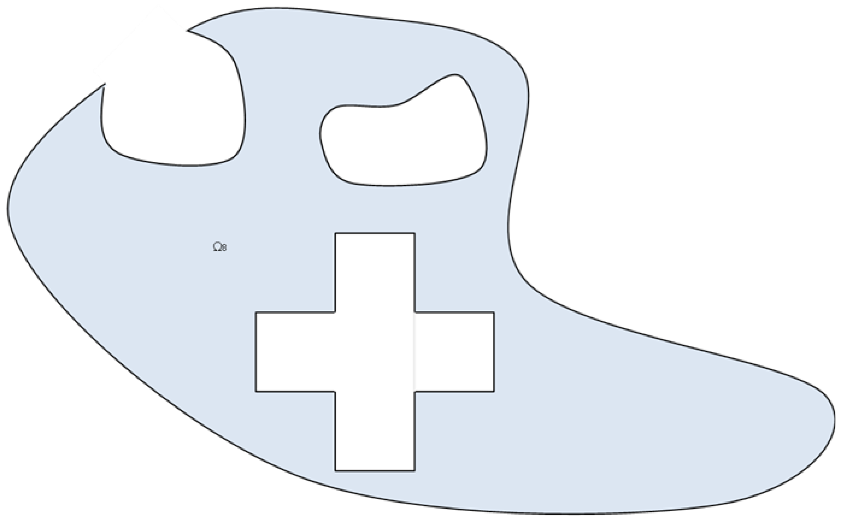
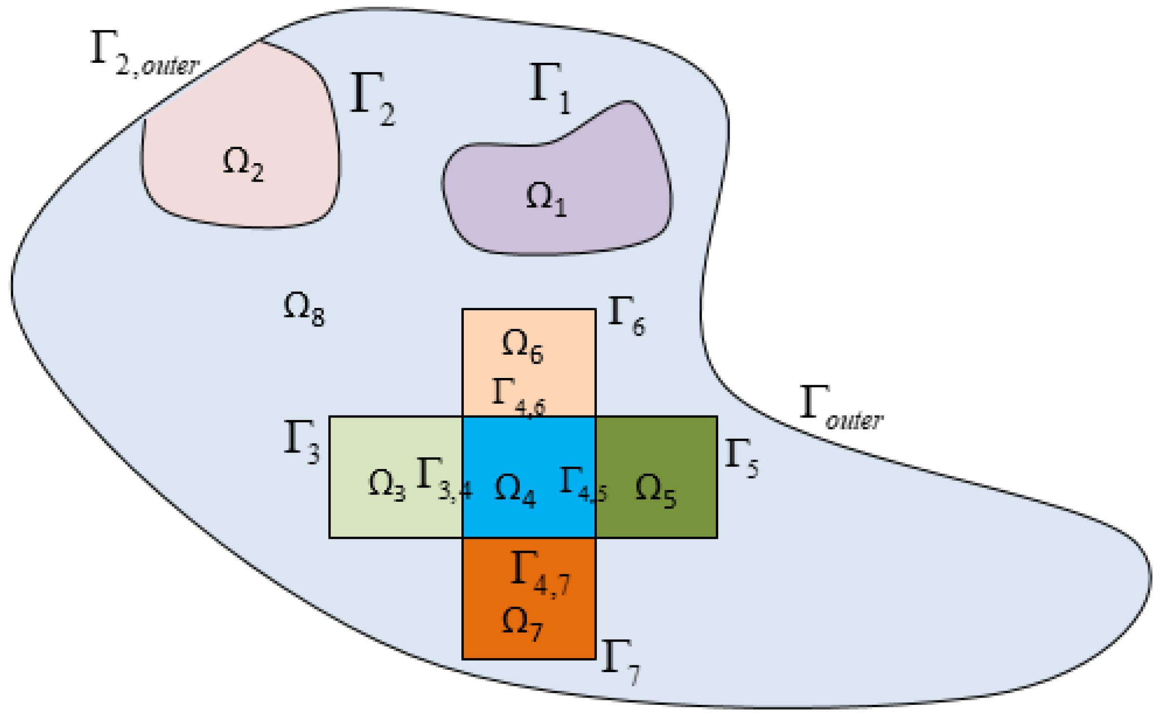
2.1. Complex Heterogeneous Reservoir Definition

A heterogeneous reservoir model consisting of eight regions representing variations of potential heterogeneities is illustrated in Figure 1. The reservoir model provides the basis of demonstrating the practical technical strategy and advantage of applying BEM in addressing a complex reservoir model. The complex model can be viewed as a real-world representation of an actual subterranean reservoir with its different reservoir flow properties for each region, which can be generally built using different information sources, such as seismic survey information and geological modeling, at the early reservoir assessment phase. For the exemplified complex reservoir model shown in Figure 1, some of the detailed reservoir descriptions and characterizations regarding the subsystems are summarized here: Γj, where j ∈ [1,7], represents the closed contour of a boundary enclosing the j-th region, and Γj,i represents the boundary/interface between the i-th region and the j-th region, i.e., Γj,I ⊆ Γi or Γj. The reservoir’s outer boundary, Γouter, (Γ2,outer is part of Γouter as the interface between Γ2 and Γouter) can be prescribed to the Dirichlet condition, Neumann condition, and mixed boundary condition to represent the real-world reservoir boundary situation. To demonstrate the proposed modeling strategy and methodology, it was assumed that the outer boundary was considered as a no-flow boundary condition in order to reach a specific heterogeneous reservoir model to be solved.

2.2. Mathematical Descriptions

The modeling of transient responses for this complex reservoir system can be achieved by decoupling and coupling the unsteady fluid flow problem for each subsystem. To achieve this, the following modeling assumptions were made:
  • Slightly compressible, single-phase fluid flow in each region was assumed.
  • Rock and fluid properties in each region were considered uniform and static.
  • Along the boundaries to be specified in the modeling process, the interfaces among all subsystems were treated as fully penetrated communicating planes with a uniform thickness of formation.
  • Any two regions with interfaces that are in hydraulic contact with no flow resistance and the interfaces/boundaries between the two regions were static.
  • Initial reservoir pressure was assumed uniform across the entire heterogeneous reservoir.
With the assumptions made above, the flow equation in a locally homogeneous region can be mathematically described as:
k j μ j ( 2 p j x 2 + 2 p j y 2 ) = ϕ j c t j p j t + k = 1 N w j q j , k δ ( x x j , k ) δ ( y y j , k ) { j | 1 j 8 ,   j I } ,
where μj, kj, and ctj are the reservoir and fluid properties in the j-th region. δ denotes the Dirac delta function, (xj,k,yj,k) is the location of the k-th source/sink of the total number of Nwj in the j-th region, and qj,k is the corresponding source/sink flow rate.

2.3. Pressure in Region 1 to 7

The pressure solution corresponding to Equation (1) for a simplified, connected domain is an integral equation given by Kikani and Horne [15] and Layne et al. [23]. With the dimensionless terms defined in Appendix A, the integral equation for any of the seven inner regions can be expressed as
θ j 2 π p D j ( x D , y D , t D ) = 0 t D d τ { Γ j M j M r e f C s r e f C s j ( G j p D j n p D j G j n ) d Γ + k = 1 N w j q D j , k G j } ,
with
θ j = 2 π i f   ( x , y ) Ω j θ j = θ j i f   ( x , y ) Γ j { j | 1 j 7 ,   j I } ,
where θj is the internal angle between two boundary elements in Region j. In Equation (2), G is the two-dimensional, free-space Green’s function and is used as a global weighting function in the integral equation given by Equation (4). Figure 2 illustrates the paths of the integral schemes for the 7 regions. It is very important to note that the p j n or G i n is considered to be “positive” when it is pointing to the outward normal direction and is considered to be “negative” when it is pointing to the inward normal direction. n is the outward-pointing normal on a boundary element, and U ( t τ ) is the unit step function.
G j ( x D , y D , x D , y D , t D , τ D ) = 1 4 π C R j C R r e f ( t τ ) D U ( t τ ) D exp [ ( x x ) D 2 + ( y y ) D 2 4 C R j C R r e f ( t τ ) D ] .

2.4. Pressure in Region 8

The pressure solution for the outer region (Region 8) is much more complex than the inner regions. Region 8 is a multiple, connected domain with complex internal interfaces and an outer boundary. Equation (2) can only be directly applied to the pressure solution within a simply connected domain with interface circling the flow domain. Appendix B presents the physical and mathematical derivation of the pressure solution for Region 8, given as:
θ 8 2 π p D 8 ( x D , y D , t D ) = 0 t D { M 8 M r e f C s r e f C s 8 [ Γ o u t e r Γ 2 , o u t e r G 8 p D 8 n p D 8 G 8 n   d Γ Γ 2 Γ 2 , o u t e r G 8 p D 2 n p D 2 G 8 n   d Γ Γ N R S P G 8 p D i n p D i G 8 n   d Γ Γ 1 G 8 p D 1 n p D 1 G 8 n   d Γ ] + k = 1 N w 8 q D 8 , k G 8 } .

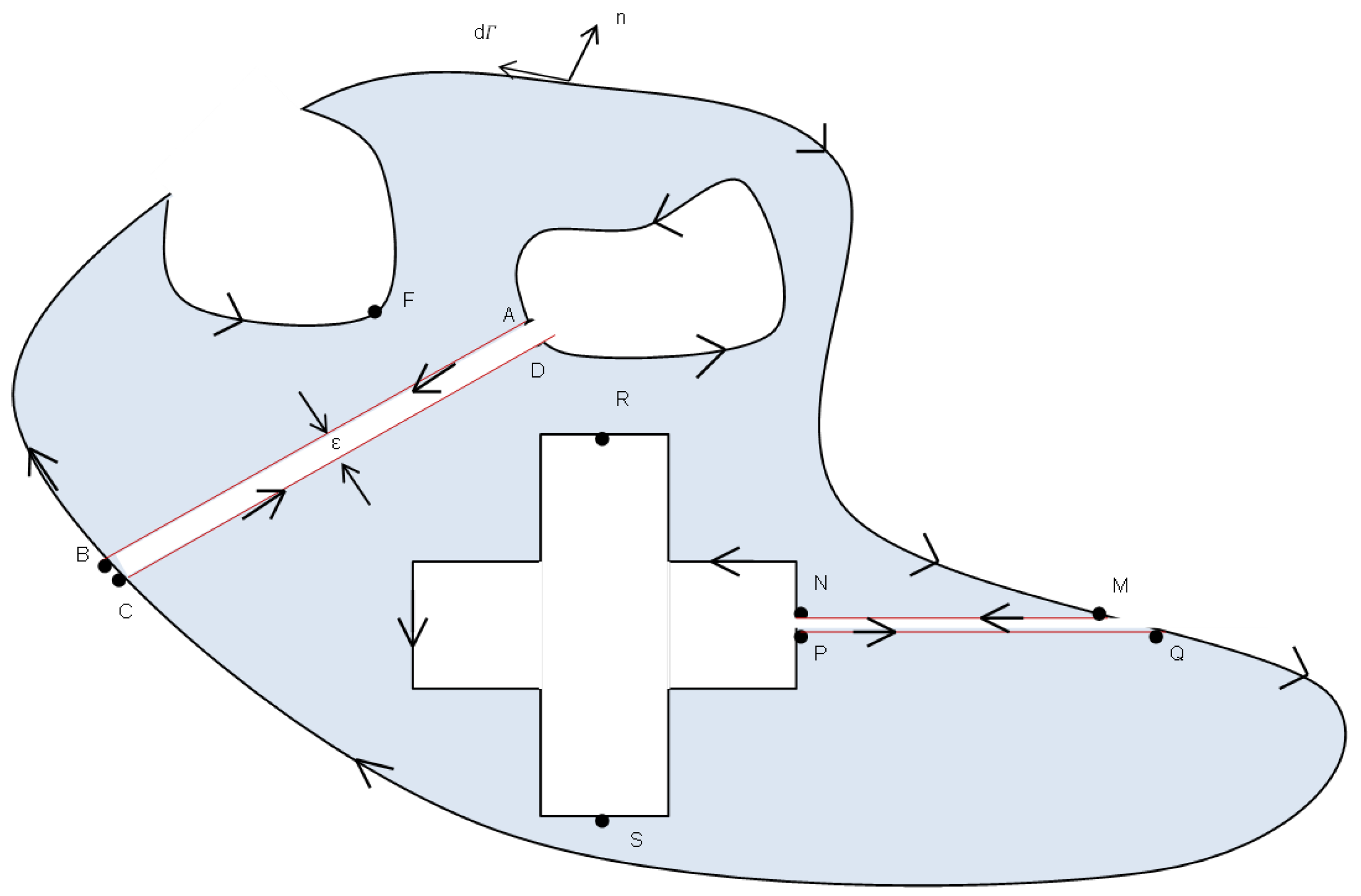
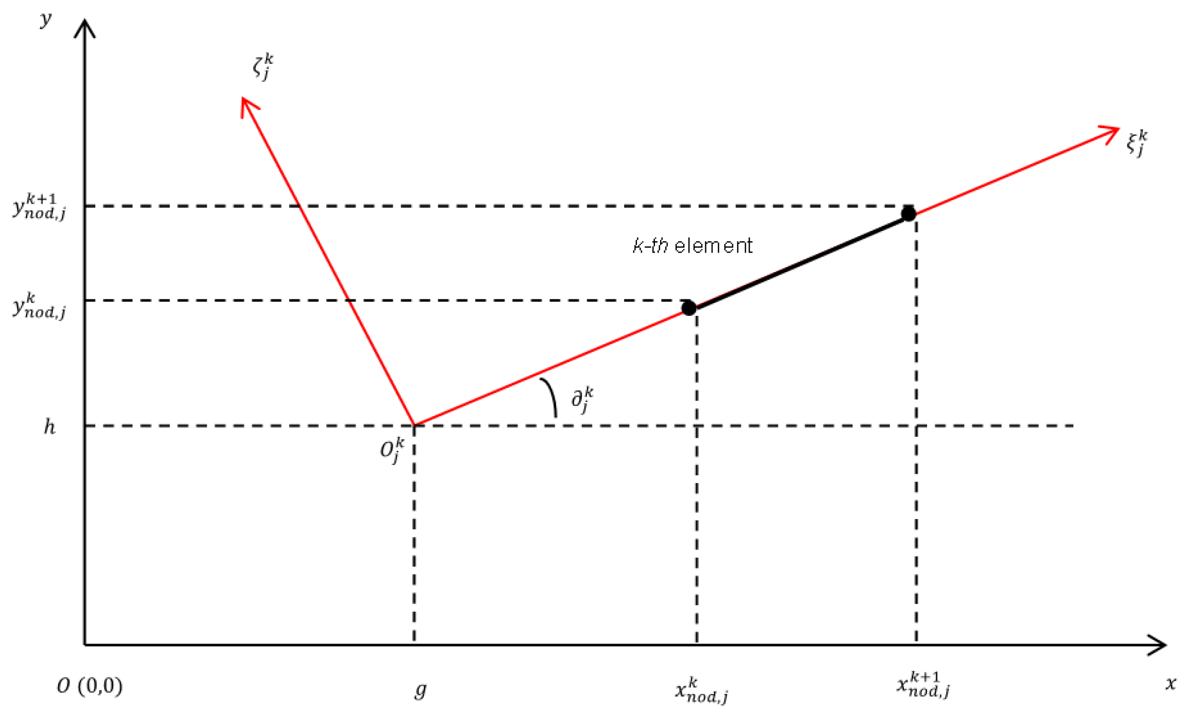
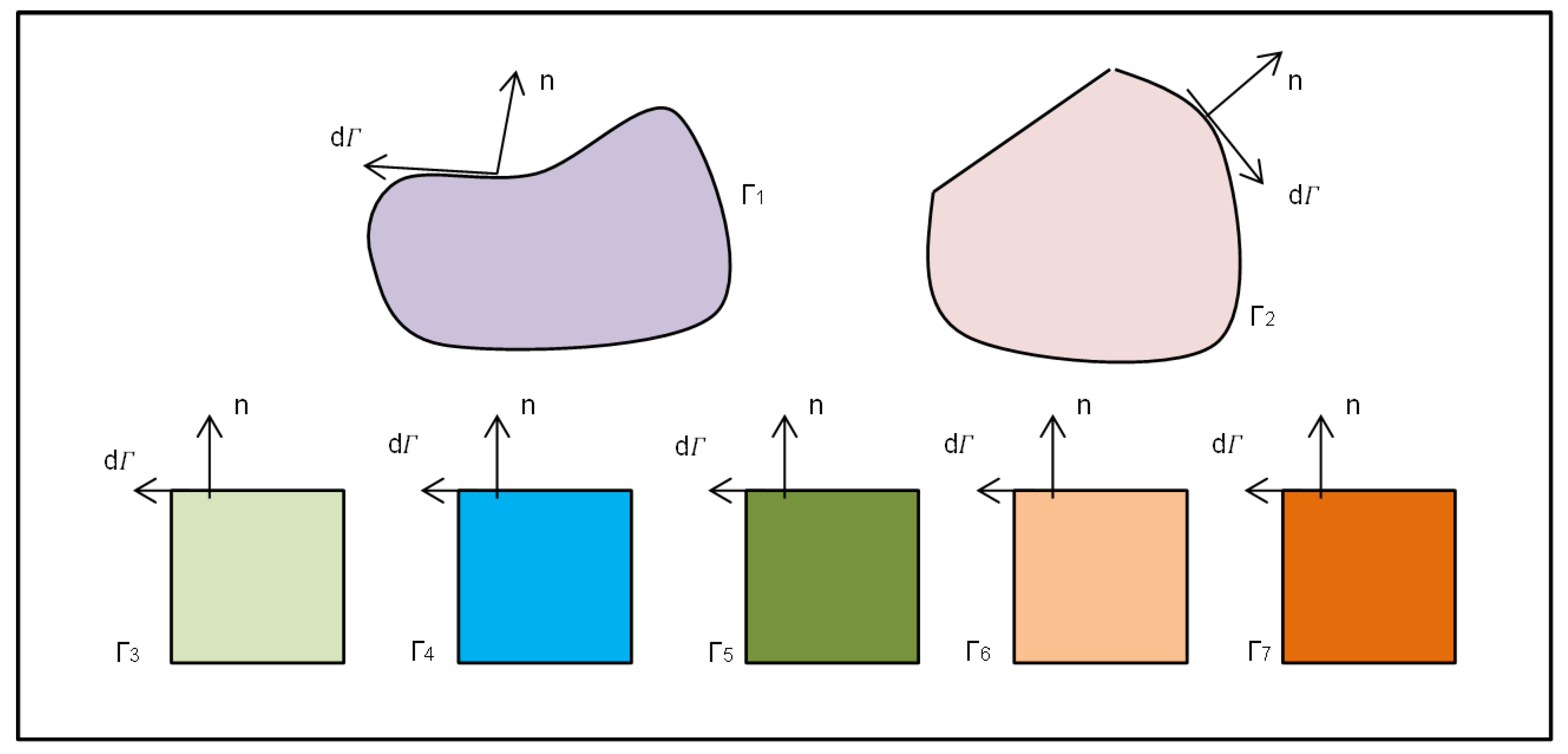
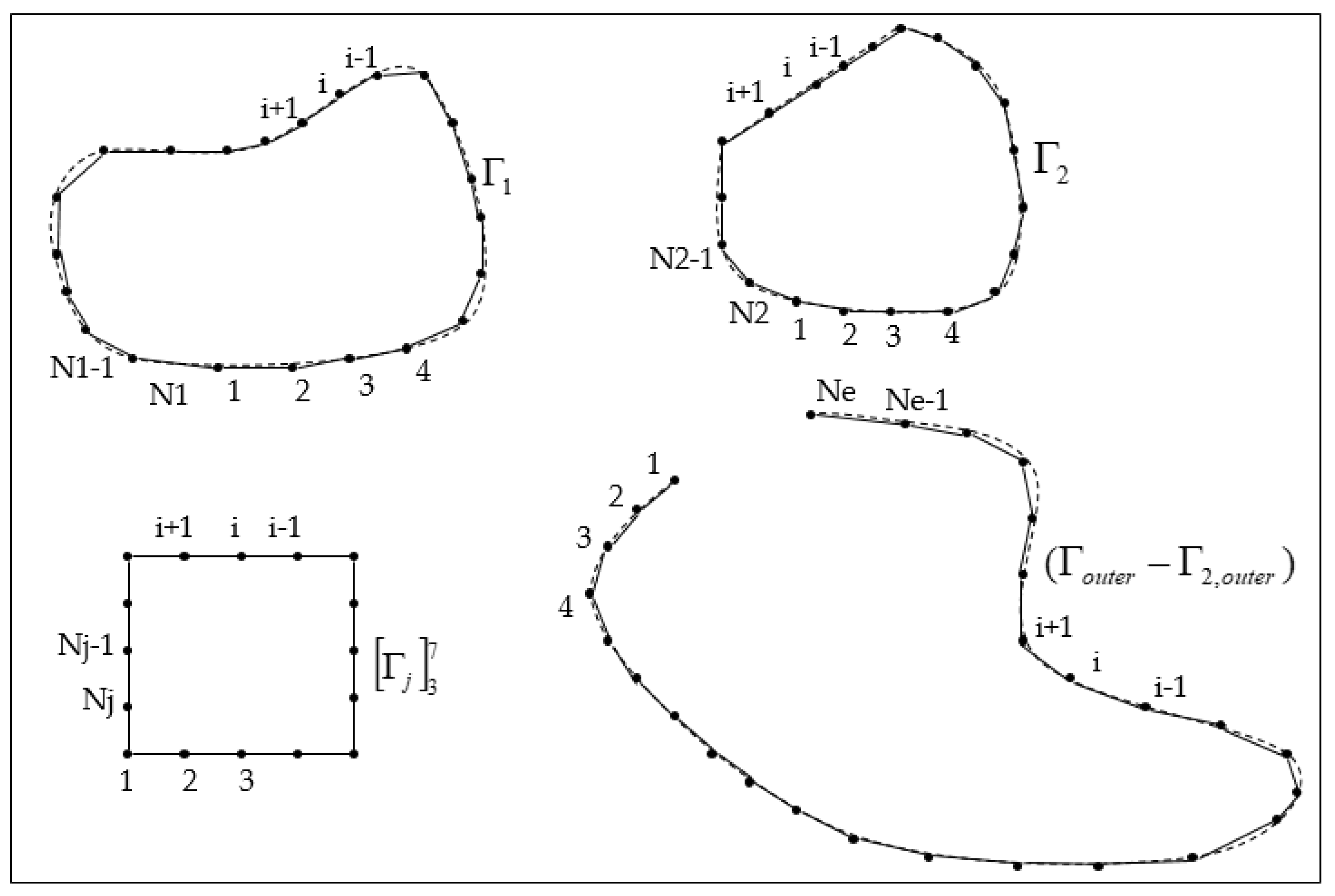
2.5. Boundary Discretization

Equations (2) and (5) require the integration of the pressure and pressure gradient, which are unknown continuous functions of position and time. To achieve numerical solution for Equations (2) and (5) for each domain, we discretized a boundary into a number of segments, referred to as “boundary elements”, by assigning nodes on the boundary. Each boundary element is formed with linear interpolations between two adjacent nodes. The pressure and the pressure gradient on each boundary element were assumed to be uniform. A boundary element with this type of discretization is generally referred as a “constant element”. The constant element is advantageous in that the integrals of the Green’s function along the boundary can be obtained analytically, resulting in improvements in calculation efficiency and accuracy. Additionally, singularity at sharp corners of adjacent elements is naturally avoided [16]. Appendix C provides the detailed derivation of the pressure expression of each region in discrete form.

2.6. Laplace Transformation

The convolution theorem is the fundamental principle for the modeling of a complicated flow process. The Laplace transform of the convolution theorem is the product of two Laplace transformed functions that are expressed originally in real time for our problem under study. The application of the convolution theorem in the Laplace domain offers great advantages in modeling. The Laplace transformation with respect to time is taken for Equations (A25) and (A26), denoted as “L[ ]”. Applying the convolution theorem, the working equation of the pressure solution in discrete form for Regions 1 to 7 by Equation (A25) in the Laplace domain becomes:
θ j k 2 π L [ p D j ( x D , y D , t D ) ] = M j M r e f C s r e f C s j { k = 1 N j L [ p D j k ζ j k ] L [ Θ ^ j k ] k = 1 N j L [ p D j k ] L [ Θ ˜ j k ] } + k = 1 N w j l [ q D j , k ] L [ G j ] ,  
and the working equation of the pressure solution in discrete form for Region 8 by Equation (A26) in Laplace domain becomes:
θ 8 k 2 π L [ p D 8 ( x D , y D , t D ) ] = M 8 M r e f C s r e f C s 8 { k = 1 N e L [ p D 8 k ζ 8 k ] L [ Θ ^ 8 k ] k = 1 N e L [ p D 8 k ] L [ Θ ˜ 8 k ] } M 8 M r e f C s r e f C s 8 { k = 1 N 2 , 8 L [ p D 2 k ζ 2 2 , k ] L [ Θ ^ 8 k ] k = 1 N 2 , 8 L [ p D 2 k ] L [ Θ ˜ 8 k ] } M 8 M r e f C s r e f C s 8 { k = 1 N N R S P L [ p D i k ζ i k ] L [ Θ ^ 8 k ] k = 1 N N R S P L [ p D i k ] L [ Θ ˜ 8 k ] } M 8 M r e f C s r e f C s 8 { k = 1 N 1 L [ p D 1 k ζ 1 k ] L [ Θ ^ 8 k ] k = 1 N 1 L [ p D 1 k ] L [ Θ ˜ 8 k ] } + k = 1 N w 8 L [ q D 8 , k ] L [ G 8 ] ,
The complex analytical Laplace transformations of Θ ^ and Θ ˜ in Equations (6) and (7) are not readily available. Onur and Reynolds provided an innovative numerical Laplace transform method [28]. An accurate and fast numerical Laplace transform scheme devised by Zhao and Thompson is applied in this study [11]. The devised scheme plays a key role in this study in modeling unsteady-state flow in a complex heterogeneous reservoir system.

2.7. Linear Matrix Equations in Laplace Domain

For each of the 7 inner regions ( j [ 1 , 7 ] ), the number of N j linear equations can be obtained in the Laplace domain by evaluating the pressure based on Equation (6), at the midpoint of every boundary element on the respective boundaries Γ j . For Region 8, N e number of linear equations can be obtained by evaluating the pressure based on Equation (7), at the midpoint of each boundary element along the reservoir outer boundary of ( Γ o u t e r Γ 2 , o u t e r ) , resulting in a set of ( N e + j = 1 7 N j ) linear equations.
In addition, the eight locally homogeneous regions interact with each other along their hydraulic contact interfaces by fluid transfer. Each region is coupled with its neighboring regions along the interface(s) based on the pressure equilibrium and rate continuity. Combined with the prescribed outer boundary condition, i.e., the no-flow boundary assumed in the beginning of this work, another set of ( N e + N j ) linear equations is established. In total, 2   ( N e + N j ) linear equations are obtained for exactly the same number of unknowns, that is, ( N e + N j ) pressure unknowns plus ( N e + N j ) pressure gradient unknowns of all the boundary elements.
By solving the set of linear equations, the pressure and pressure gradient of each boundary element can be obtained in the Laplace domain and substituted into Equation (6) or Equation (7), such that the pressure at the desired location within the reservoir can be obtained. The pressure, pressure gradient, and rate solutions in the Laplace domain can subsequently be inverted to the real-time domain using the Stehfest inversion algorithm [29].

3. Model Validity and Results

3.1. Scenario 1: Fully Compartmentalized Reservoir

The pressure and rate behaviors of the well to be presented in the following theoretical cases are under either constant rate or constant bottom-hole flowing pressure (BHFP) conditions, accordingly. Figure 3a assumes a roughly configured reservoir model with a box-shaped, no-flow outer boundary. The reservoir consists of 25 irregularly shaped compartments/regions, and each compartment is numbered accordingly. The reservoir is produced by a vertical well located in Region 13, represented by a source point.

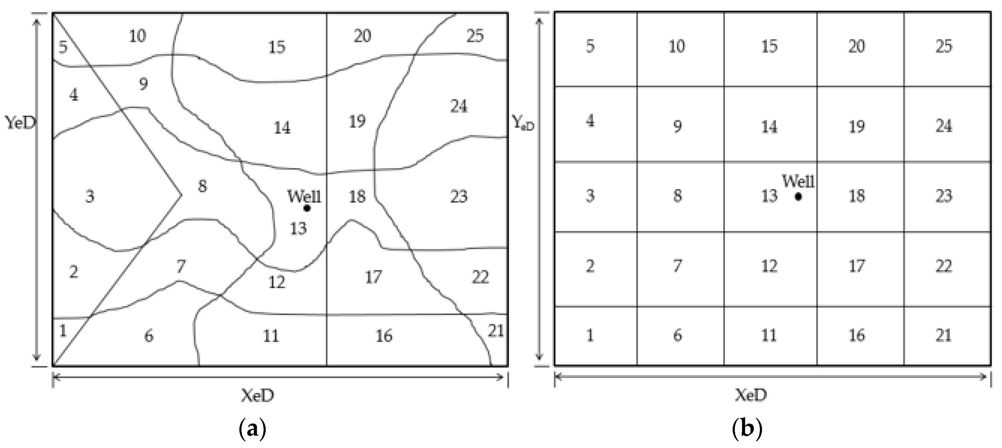
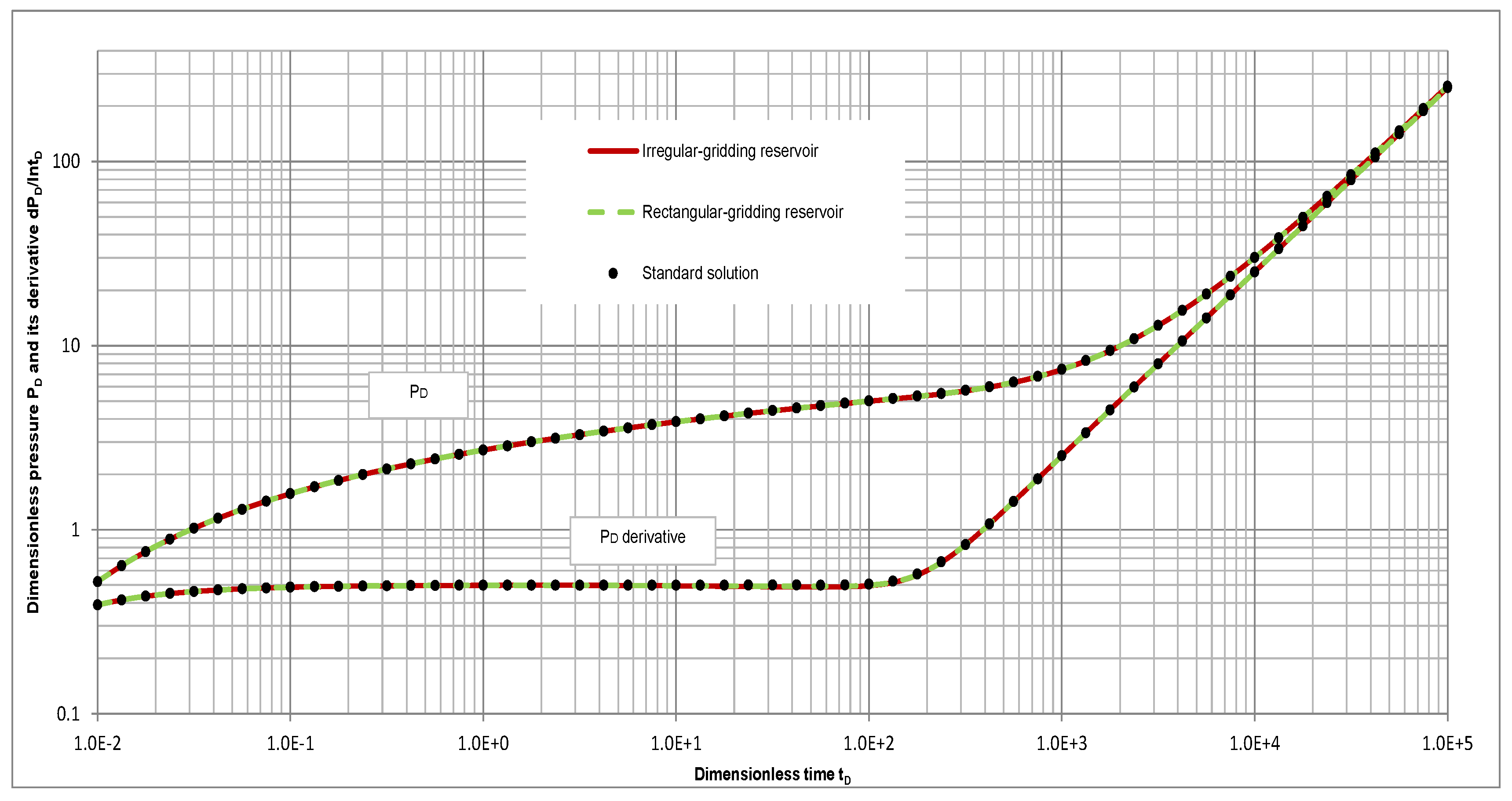
3.1.1. Scenario 1—1: Standard Reservoir with Discussion on Gridding

One of the greatest advantages of BEM is that the method is capable of handling fluid flow in bounded reservoirs with irregular boundaries in a comparatively easy and convenient manner as presented and discussed in this paper. This means that the definition of geometric regions is mainly based on the geological feature of reservoir rocks. Thus, this BEM scheme offers a mesh-free computing process because only segmental discretization along boundaries is required. Furthermore, one’s attention should be drawn to the fact that neither BEM nor SSFM strategies need gridding within each homogeneous region because the reservoir system has been separated and integrated with an analytical strategy to maintain hydraulic communication among different regions of the reservoir system, thus to establish solution with near analytical accuracy, regardless of boundary shapes. The regions enclosed by the grid-like lines and curves in Figure 3a,b are for geological description purposes only, i.e., the reservoir properties for each region can be input accordingly based on an actual geological reservoir model to match. Because of the gridding effect on solutions for finite difference and finite element simulation, there exist well-known challenges that cause numerical inaccuracy in solution; thus, it is necessary to examine how the boundary discretization schemes affect the solution accuracy for BEM and SSFM strategies under homogenous and heterogeneous reservoir conditions.
To understand the boundary discretization effect in a homogeneous reservoir case, a reservoir system is regionalized into 25 irregular regions and 25 regular, rectangular regions, as illustrated in Figure 3a,b, respectively, with each region defined as homogeneous in mobility and storativity. BEM can then be applied to generate the solutions. For a homogeneous reservoir in a single, rectangular-shaped reservoir, the pressure solution can also be described with the well-known standard solution given by Gringarten et al. [2] and Carslaw and Jaeger [1], as described in Equations (8) and (9) for efficient early and late time-computing, respectively. In theory, the solutions generated by the BEM strategy and the standardized solutions generated by traditional strategies, such as the imagine method, must overlap each other with nearly unnoticeable differences. The results shown in Figure 4 confirm this expectation. This result provides supporting evidence that the boundary discretization scheme in BEM does not affect the accuracy of the pressure and the pressure derivative solutions.
p D ( x D , y D , t D ) = 0 t D 1 2 t D · { n = exp [ ( x x + 2 n x e ) D 2 4 ( t τ ) D ] + exp [ ( x + x + 2 n x e ) D 2 4 ( t τ ) D ] · n = exp [ ( y y + 2 n y e ) D 2 4 ( t τ ) D ] + exp [ ( y + y + 2 n y e ) D 2 4 ( t τ ) D ] } d τ D ,
p D ( x D , y D , t D ) = 0 t D   1 X e D [ 1 + 2 n = 1 exp ( n 2 π 2 t D X e D 2 ) cos ( n π x w D X e D ) cos ( n π x D X e D ) ] · 1 Y e D [ 1 + 2 n = 1 exp ( n 2 π 2 t D Y e D 2 ) cos ( n π y w D Y e D ) cos ( n π y D Y e D ) ] d t D .

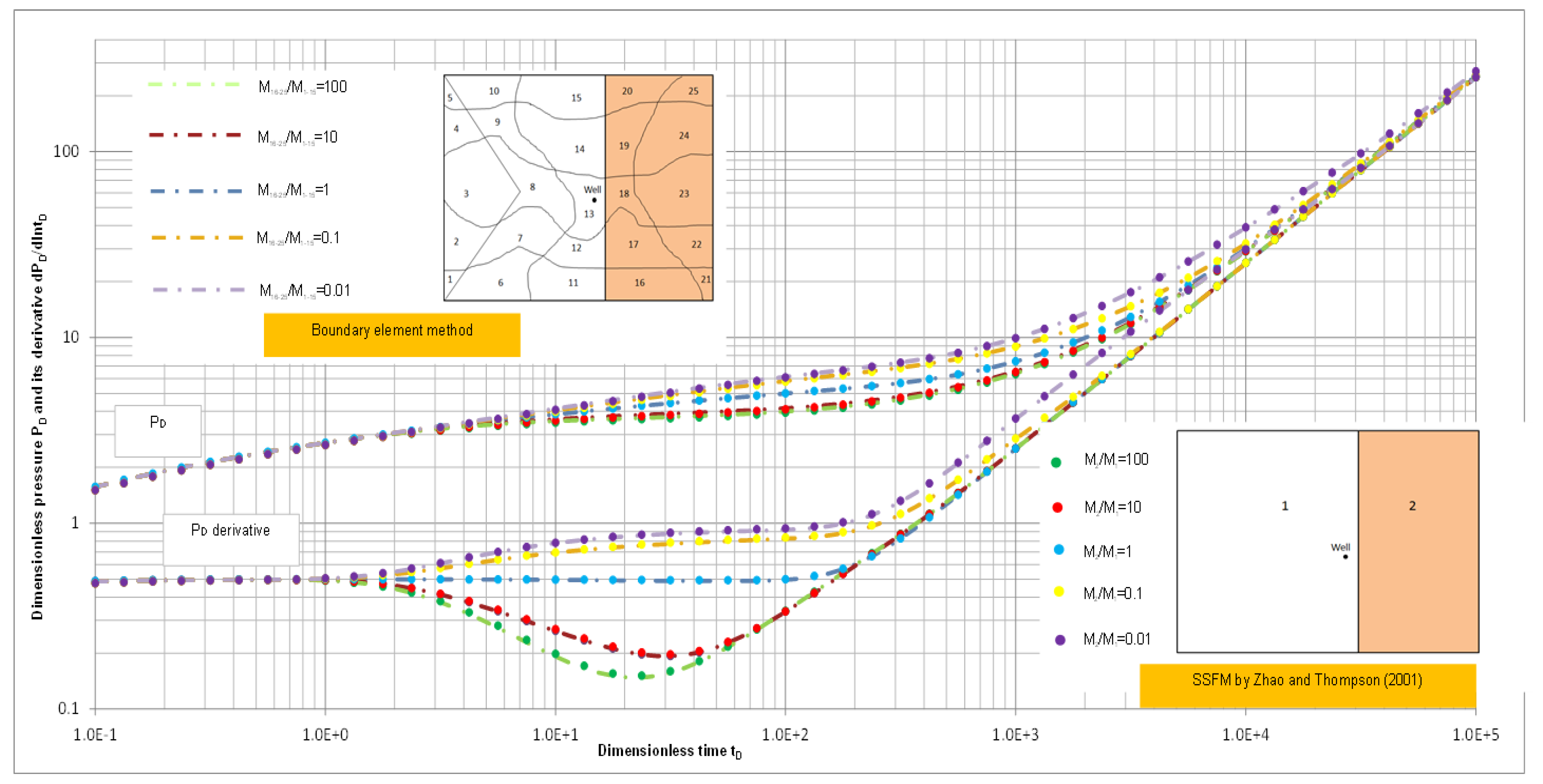
3.1.2. Scenarios 1—2: Linear Composite Reservoir

To validate the accuracy of the solutions for a heterogeneous reservoir generated by the BEM proposed, we confirmed our results against the solutions using SSFM provided by Zhao and Thompson [10], using the same regionalized scheme as shown in Figure 3a. To model a linear composite reservoir with the heterogeneous reservoir schematic shown in Figure 3a, the 1st to the 15th compartments are set to have uniform mobility; however, the 16th to the 25th regions contain a different value for each heterogeneous reservoir case computed. The heterogeneous reservoir consists of two composite parts, as illustrated in Figure 5. The cases with different mobility ratios from Area 2 to Area 1 are computed, and the solutions from the 2 methods have very good agreement.
Once it is confirmed that the BEM strategy proposed offers similar results to those from SSFM, our technical confidence is enhanced, and the technical horizon of the BEM strategy expands significantly. One may realize that the scenario shown here only verifies the accuracy of the BEM strategy for heterogeneous reservoir simulation; its full application capacity can be revealed through its application for a full field-scale heterogeneous reservoir as proper heterogeneity can be mapped into each irregular region accordingly if there is a need.
Generally speaking, BEM preserves the analytical nature of the solution as it retains the free-space Green’s function that governs the differential flow equation as a global weighting function. BEM also largely eliminates problems normally encountered in simulations, such as numerical dispersion, grid shape, and grid orientation.

3.2. Reservoir with Multi-Scale Heterogeneities

The purpose of Scenario 2 is to investigate the three types of reservoirs with different geological features: a naturally fractured reservoir with 2 different fracture distributions and a fluvial reservoir with meandering sandbars deposited within the fluvial channels. By using BEM to treat natural fractures as the heterogeneity of the geological media consisting of unique geometries and flow characteristics, such as the length, aperture, and height; the permeability; and the storativity. The natural fractures are thereby modeled in a more realistic and more physically driven manner. The tedious and complex gridding cells needed around natural fractures in other simulation methods become unnecessary, thus the BEM modeling strategy is more correctly constructed in physics, much more reliable, and easier to implement [30,31]; this is especially true for a single-phase process. For multiphase flow, we admit that it is still challenging, and further effort is demanded. The three scenarios considered are: a well produces between two parallel, natural fractures; a well produces near two intercepting, natural fractures; and multiple wells produce in a heterogeneous reservoir with multiple sandbars within a meandering, fluvial channel.

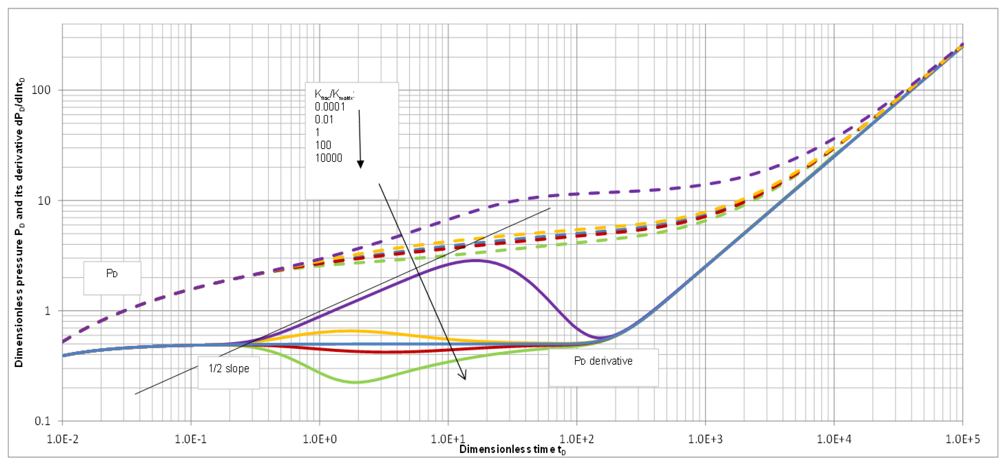
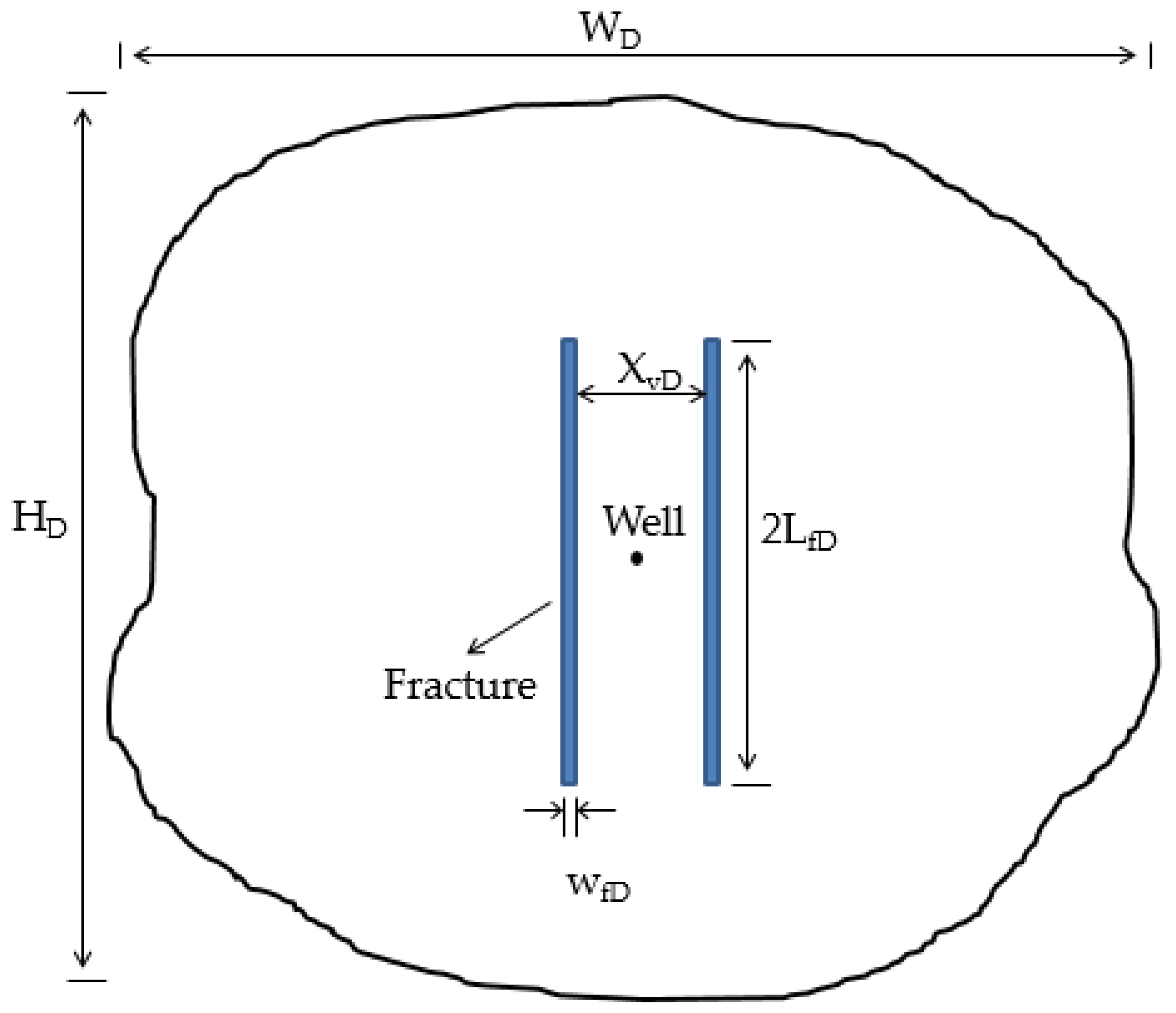
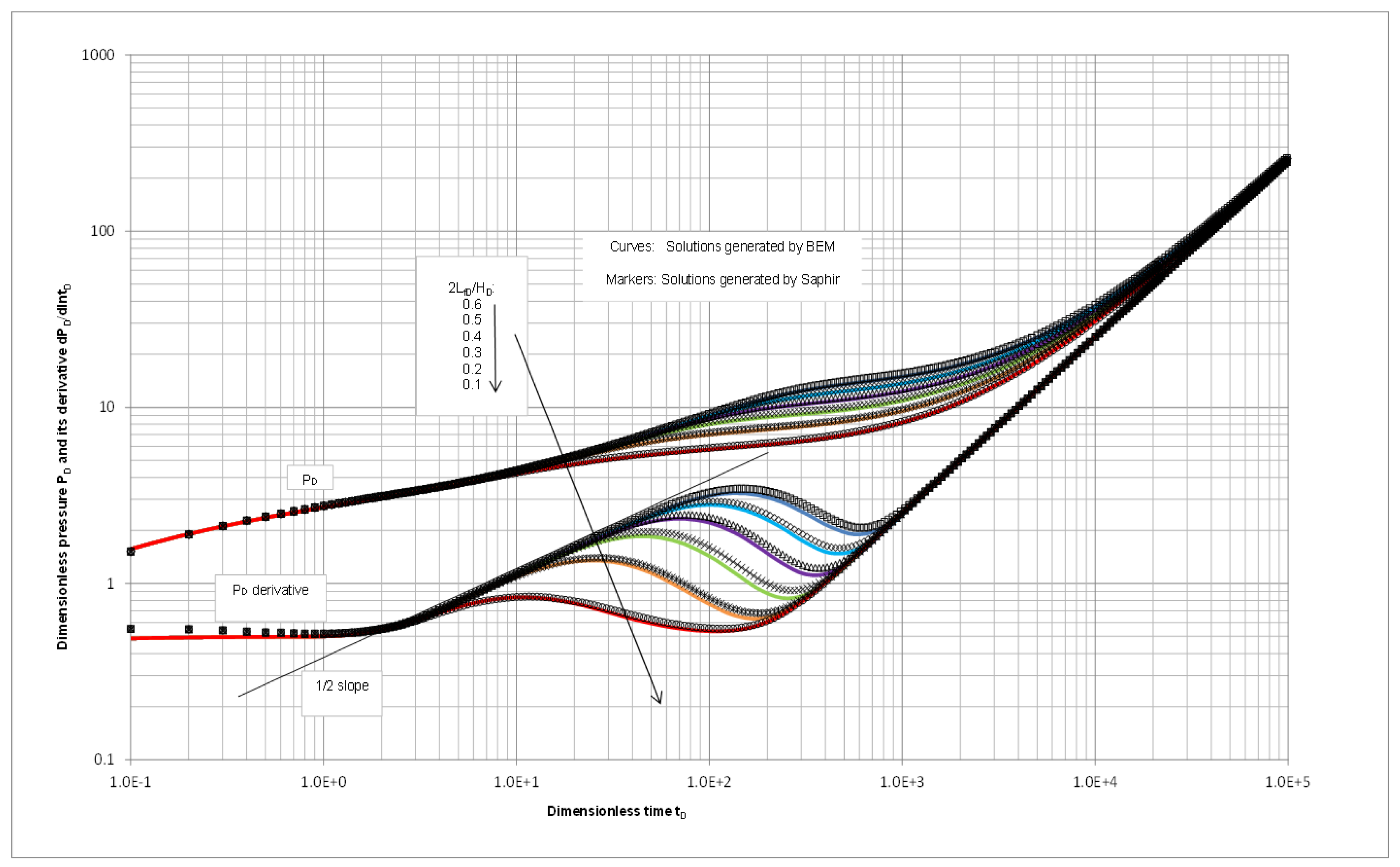
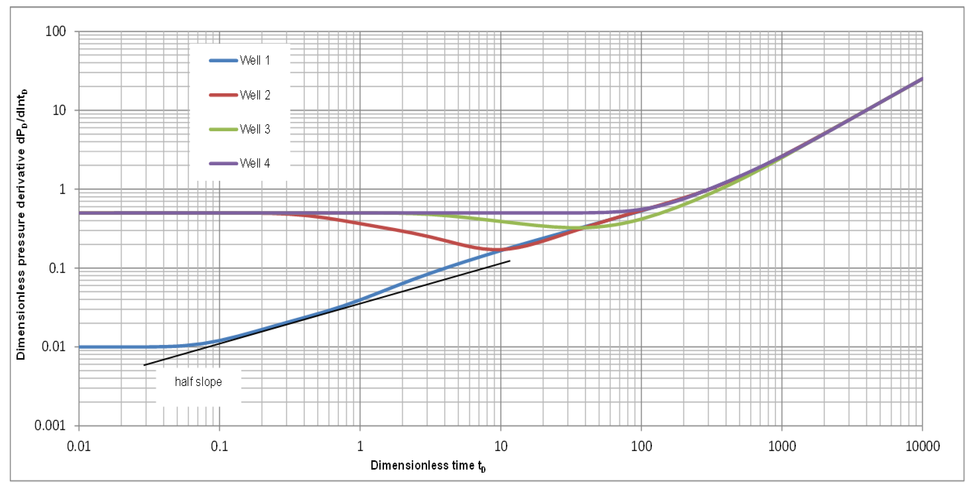
3.2.1. Scenario 2—1: A Reservoir with Two Isolated, Parallel, Natural Fractures

Scenario 2—1 studies the well response influenced by two parallelly embedded, isolated, natural fractures that are located within a reservoir with a no-flow outer boundary, as shown in Figure 6. The shape of the outer boundary is purposely defined with an irregular geometry to demonstrate the technical capacity of the BEM strategy. The natural fractures, with a range of parameter variations, are intended to be examined. The pressure- and rate-transient behaviors of the well are examined under various levels of fracture conductivity that is reflected by the permeability ratios of fracture permeability-to-formation matrix permeability. Note that the two isolated fractures are assumed to have the same flow properties, and the well is at the mid-point between these two fractures in order to simplify this ideal case.
Figure 7 and Figure 8 show the pressure and the rate behaviors, respectively, when the well is producing between two parallel, sealing faults, which are described by setting natural fracture permeability extremely low as k f r a c / k m a t r i x = 0.0001 , with W D = 50 , H D = 50 , w f D = 0.01 , and X v D = 5 . Pressure and pressure derivative solutions generated by the use of the commercial numerical modeling software Saphir are also shown in Figure 7. The results generated by BEM and the Saphir software show good agreement. Further examination indicates that BEM offers more accurate outcomes. The geological channel-flow feature has been clearly exhibited on the pressure derivative with 1/2 slope when 2 L f D H D > 0.2 . However, the declining 1/2 slope trend is not so obviously shown in the rate decline-curve, even when 2 L f D H D > 0.6 is reached, as illustrated in Figure 8. A comparison between the pressure derivative curves with the rate-decline curves suggests that the rate-decline curve is not as sensitive to the geological features of the reservoir. Generally speaking, when pressure-transient hits fault tips, pressure derivative starts to go downward as fluid beyond the fault tips flows into the channel before the outer no-flow boundary is felt.
In addition, the effect of the permeability of natural fractures is also examined in this scenario. The results, in terms of transient pressure and rate, presented in Figure 9 and Figure 10, have a fixed fracture width of WfD = 0.01 and fracture lengths of 2LfD = 10, XvD = 2, WD = 50, and HD = 50. As illustrated in these two figures, the natural fractures clearly affect pressure- and rate-transient response when the fracture is 10,000 times more permeable than the formation rock. The impact of the natural fracture on well behavior is even more pronounced when the fracture is 10,000 times less permeable than the formation, acting as non-conductive faults.
In order to determine the source of the results shown in Figure 9, the flux profiles for the left-hand-side (LHS) and the right-hand-side (RHS) faces of the fracture are shown in Figure 11. Note that the flux profiles are for only one fracture. The flux profiles at t D = 1 ,   10 , and   100 for highly conductive fractures with k f r a c / k m a t r i x = 10 , 000 are presented in Figure 12. It is observable that, for the LHS face of the fracture, its outer portions have negative flux values, which means that this conductive fracture is passing fluid quickly toward the well and also extracting fluid around the LHS face’s outer portions into itself. The extracted fluid flows along the fracture, as indicated by the red-colored arrows in Figure 11a, into the middle portion of the fracture where it is eventually produced out of the LHS face of the fracture, indicated by the positive flux values. On the other hand, the flux on the RHS of the fracture is always flowing into the fracture, as indicated by its positive flux values. When the fracture is much less conductive, fractures only pass as much fluid they can receive directly from the RHS to the LHS, as illustrated in Figure 13. The observations made above using BEM are consistent with the observations of Zhao made by implementing SSFM [32]. Therefore, the outcome from this independent BEM simulation is correct. This enhances our technical confidence in developing a BEM-based simulation package.

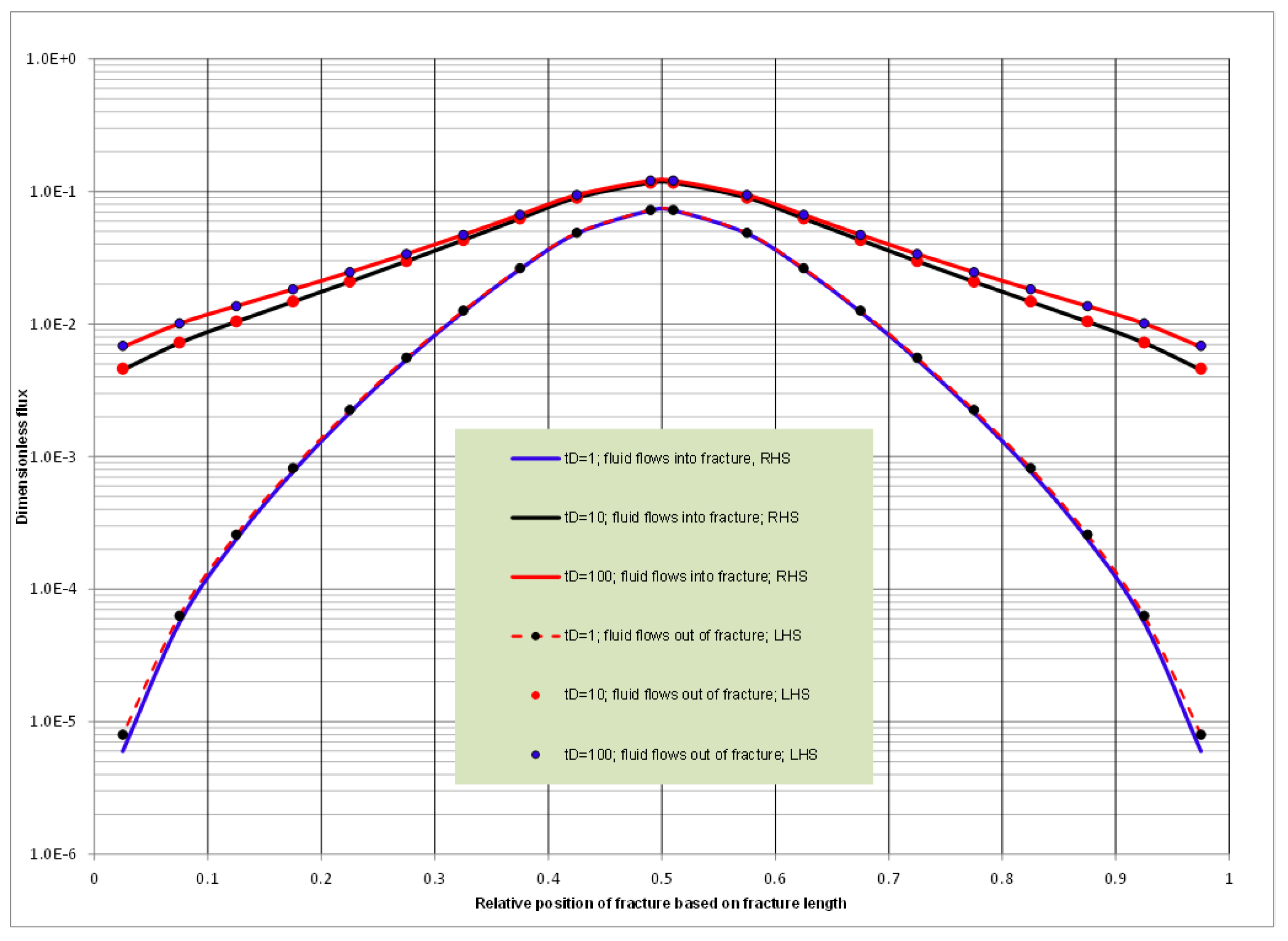
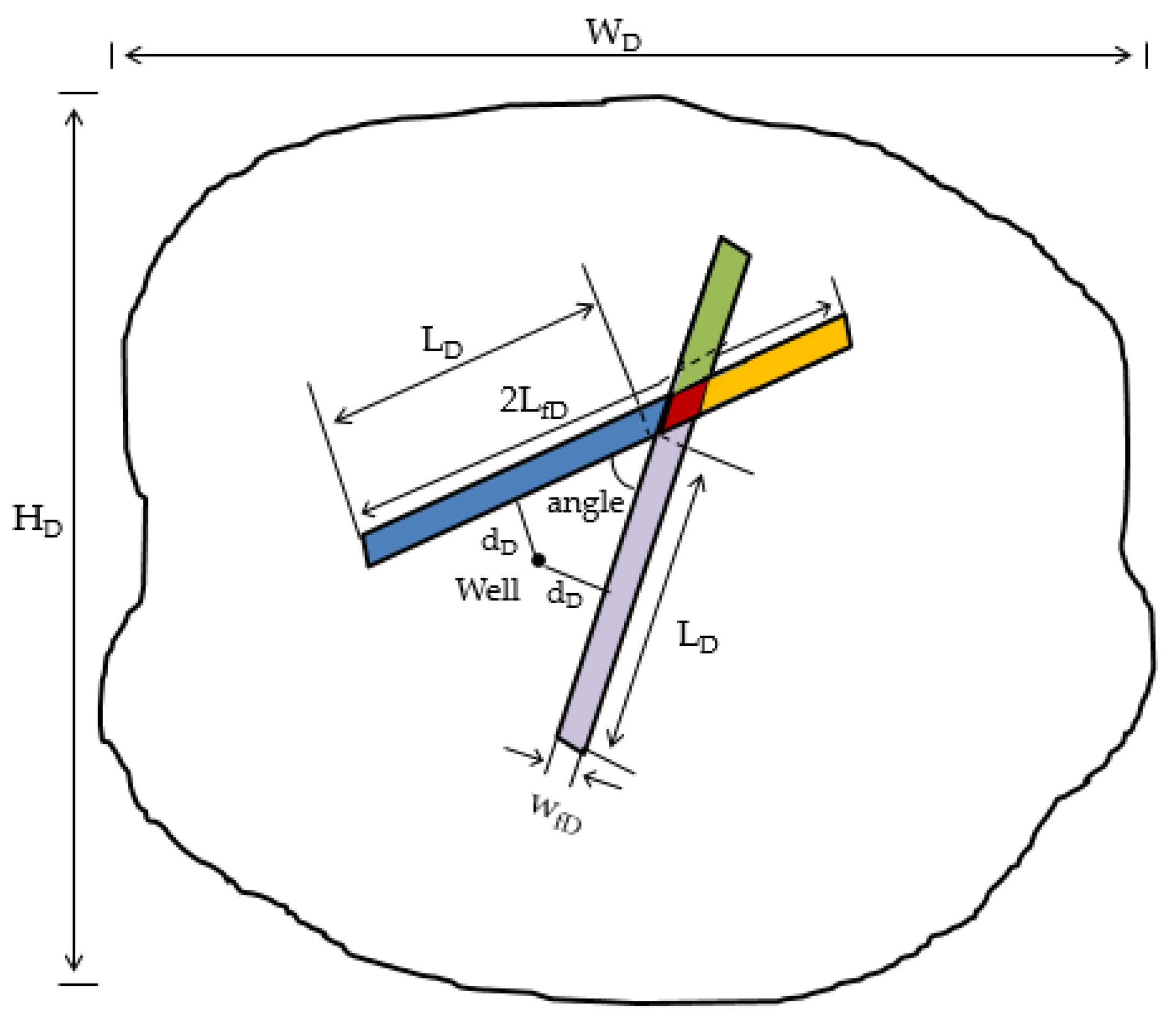
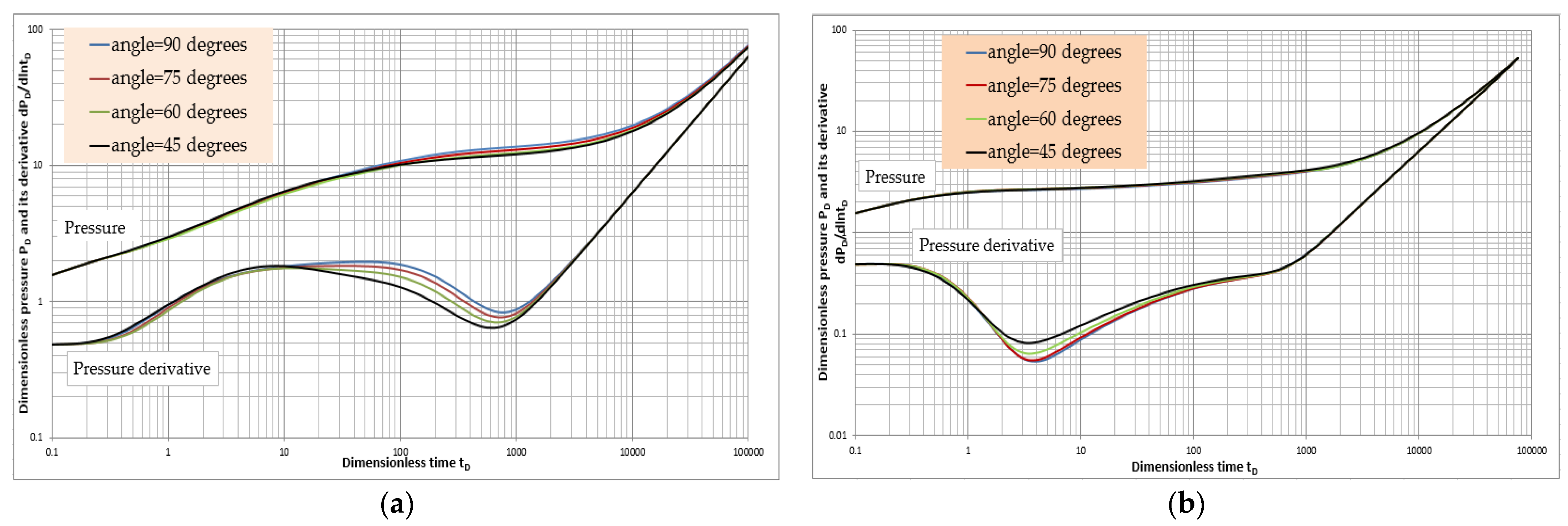
3.2.2. Scenario 2—2: A Reservoir with Two Isolated, Crossing, Natural Fractures

The effect of two isolated crossing natural fractures on well behaviors is investigated in this scenario, assuming fluid properties remain unchanged. Figure 14 presents the schematic of the naturally fractured reservoir. Two isolated, crossing fractures intercepting each other at various angles, forming a parallelogram of the conjunction area. The reservoir is modeled by describing the fracture network consisting of the five regions, represented by different colors. The purpose of using colored regions is to clearly demonstrate the individual sections of this fracture network. The flow properties of these regions can be assigned with different values if needed.
The effect of the different angle between these two sealing faults with k f r a c / k m a t r i x = 0.0001 is examined at 90 ° ,   75 ° ,   60 ° , and 45 ° , with L D / 2 L f D = 3 / 4 , and d D = 1 . Figure 15a shows that, at the time roughly after tD > 10, a wider, included angle causes slightly greater pressure drop, which responds to the fact that a wider angle results in a larger extent to allow the sealing faults to impede fluid flow towards the wellbore, and the fluid has to bypass the sealing faults. It is noticeable that, when fractures are orthogonal at 90 ° angle, the pressure derivative increases and stays at d p D / l n t D = 2 . This is due to the well-known derivative doubling phenomena caused by a sealing fault’s influence, which occurs for a specific period of time before it drops as a result of the fluid beyond the faults starting to flow towards the wellbore.
If the fracture geometry setting remains the same and only the fractures become very conducive with a permeability ratio of k f r a c / k m a t r i x = 1.0 × 10 4 , it is observable that, at dimensionless time after tD > 1.2, a wider included angle causes a slightly smaller pressure drop with a decreased derivative value (Figure 15b). This is due to the fact that the fracture setting with a wider angle covers a larger extent to promote fluid flow towards the wellbore. The detailed derivative characteristics identified in this scenario show how a large-scale geological feature can be quantitatively determined.

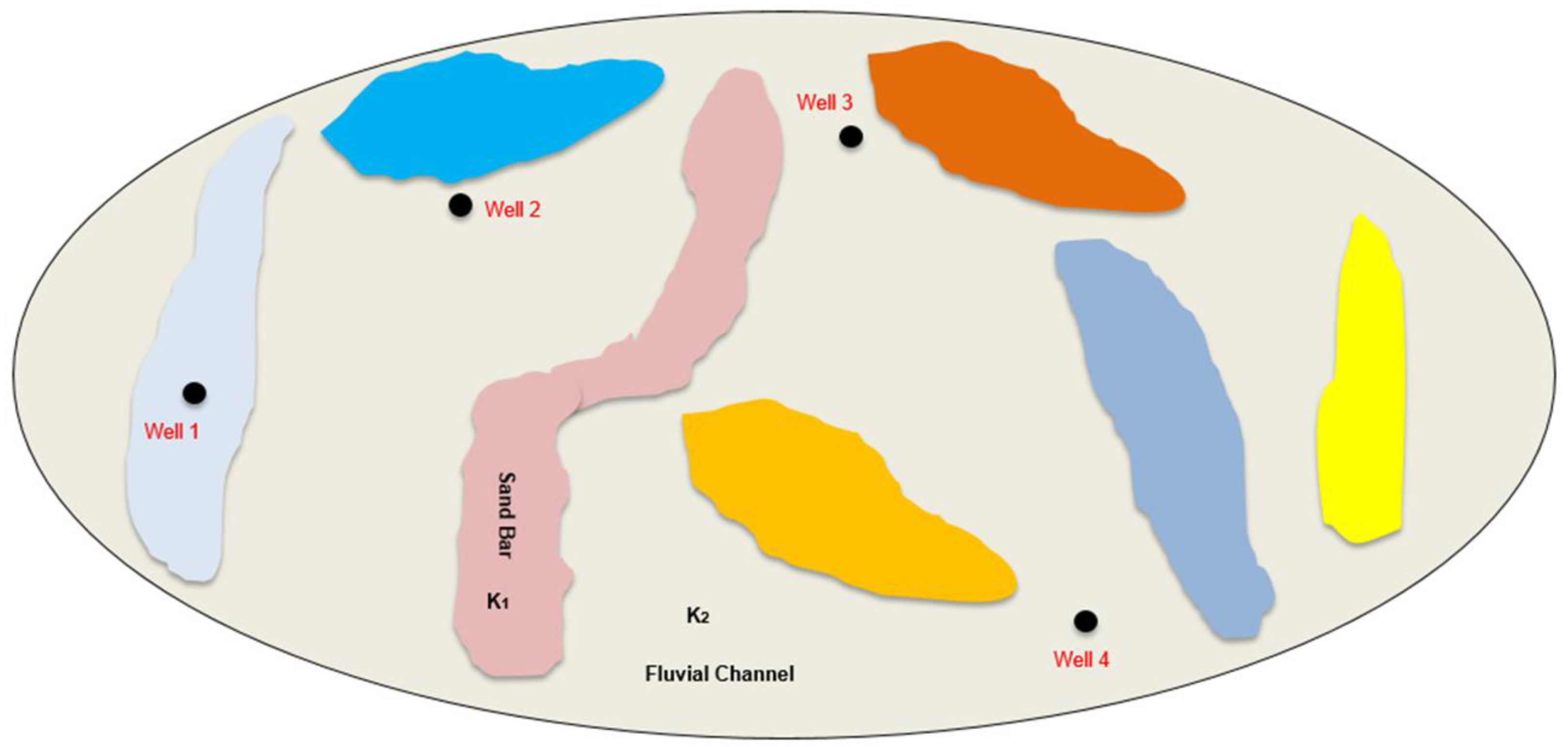
3.2.3. Scenario 2—3: Reservoir with Sandbars in Fluvial Channeling

The fluvial reservoir scenario models the transient behaviors of multiple wells completed in geologically complex environments. A schematic of a geologically complex reservoir is illustrated in Figure 16, with K1 representing the permeability inside the sand bar while K2 representing the permeability of the fluvial channel. The layout of the reservoir is represented as a fluvial channel with an elliptical outer boundary under braided fluvial sedimentation consisting of seven irregularly shaped sandbars. Note that all of the sandbars were assumed to have the same storativity and mobility. In a fluvial channel system, sandbars are usually the “sweet spots” and are the target locations to complete wells due to the highly transmissive sediments. The application of seismology in delineating sandbars in deep reservoirs has many limitations due to the lack of high-resolution information to determine the spatial extent and distribution of the sediments. However, interpretation of the pressure data from such a reservoir can provide an estimate of the relative spatial relationships between the well and the fluvial system.
The pressure derivatives of the 4 vertical wells, where Well 1 is placed in a sandbar and the other 3 wells are located in the fluvial channel (Wells 2 and 3 are located spatially closer to a sandbar as compared to Well 4) are shown in Figure 17. In this scenario, the permeability ratio of the sandbars to the fluvial channel is set at 50. Pressure derivative profiles of Wells 1, 2, and 3 clearly reflect the effect of reservoir heterogeneities. The pressure derivative of Well 1 increases quickly early when its pressure transient hits the sandbar’s boundary. Subsequently, the characteristic of the channel flow with a half slope is evolved due to the contrast in permeability between the sandbar and the outside fluvial channel environment. The transition is due to the change of permeability from the sandbar and the fluvial channel sediments, where the fluid that in the less-permeable fluvial channel has difficulty flowing into Well 1 and the production is mainly provided by fluid in the sandbar; this is especially true early in the flow period. Wells 2 and 3 are affected by the surrounding sandbars with a decline in their pressure derivatives, while Well 4 is only slightly affected due to the distant sandbars near it.
Although the simple reservoir settings of the 3 scenarios in this example are insufficient to comprehensively examine the effect caused by all types of natural fracture networks or fluvial systems, the main purpose of the examples is to showcase the technical capacity of modeling natural fracture networks or fluvial systems and the high level of solution accuracy using the proposed BEM modeling strategy. Because tight oil/gas reservoirs have been increasingly playing an important role in oil/gas production, with multi-stage fractures being implemented on horizontal wells, there is a need to understand and analyze complex fracture networks as formed by connections of hydraulic fractures and natural fractures. The proposed BEM modeling technology provides a powerful tool to simulate complex, natural networks. It can address multiple complex fracture networks. The only limitation of the method is that it is subject to the available computing resources.

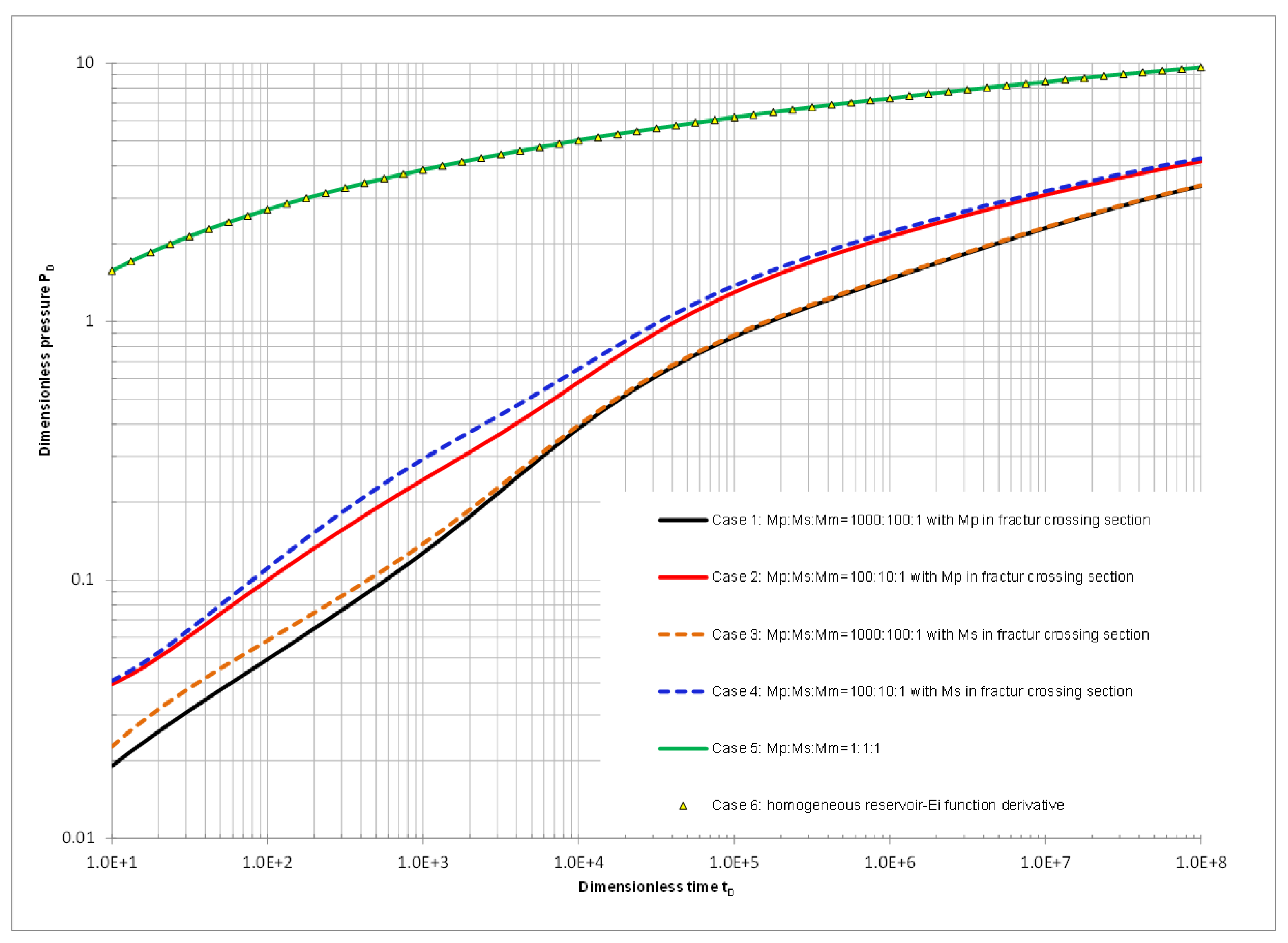
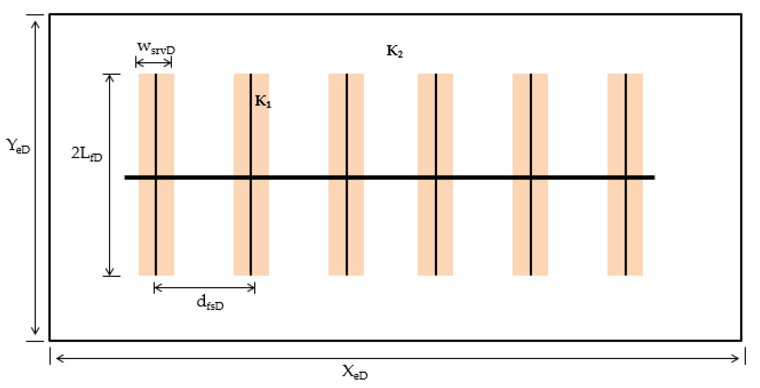
3.3. Scenario 3: Enhanced-Fracture-Region (ERF) Model

Stalgorova and Mattar proposed a physical model to address multi-stage hydraulically fractured horizontal wells (MHFHW) [33]. This model provides an excellent attempt to capture the effect of an “enhanced” permeability region in the vicinity of each main fracture by assigning a local, stimulated reservoir volume (SRV) with a higher permeability than the formation matrix’s permeability. The local SRV can be considered as inclusive of fracture branching/complex networks or densely distributed natural fractures. However, a comprehensive set of solutions for this model has not been fully established. In reality, a region of “reduced” permeability may also be generated in the vicinity of fracture, due to the fracturing fluid induced formation damage and the effective hydrocarbon permeability reduction caused by the multiphase flow environment under the condition of high fracturing fluid saturation. For the possible phenomena within this scenario, the effects of local SRV permeability versus matrix permeability need to be comprehensively studied.
The schematic of the physical model with local SRVs in this scenario is shown in Figure 18. The six-stage transverse fractures are evenly spaced along the horizontal wellbore. It is assumed that each stage has only one main fracture, and fractures can be easily placed unevenly along the wellbore when necessary. With the flexibility of the BEM strategy, it is of great technical benefit to compute and analyze pressure or rate behaviors when a local SRV around a fracture has various levels of permeability or various sizes.

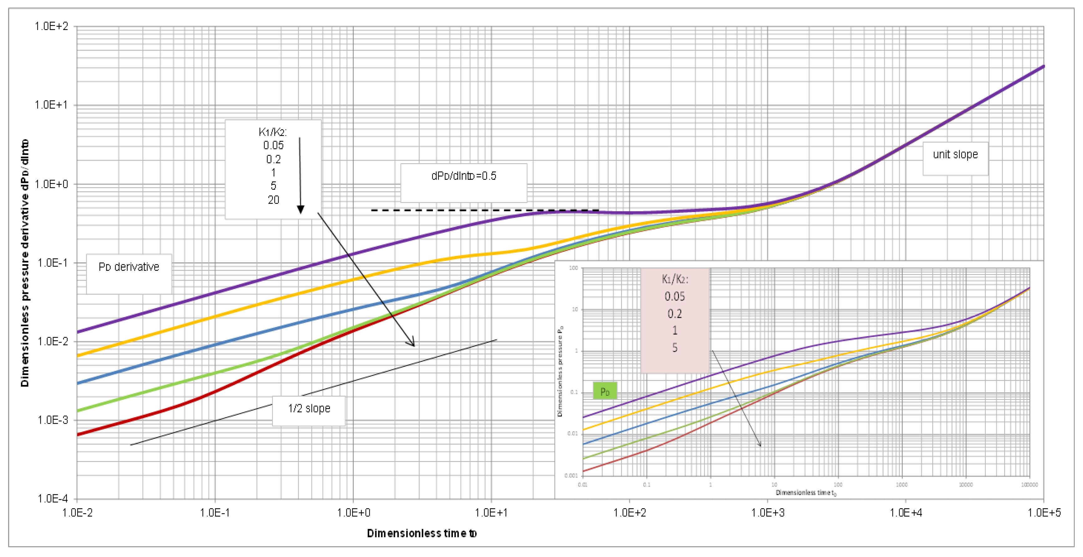
3.3.1. Effect of Local SRV Region Permeability

Pressure- and rate-transient behaviors of MHFHW are shown in Figure 19 and Figure 20, respectively. In Figure 19, early formation linear flow with 1/2 slope is exhibited for different permeability ratios of k 1 / k 2 . However, when the k 1 / k 2 ratio is larger than 1, indicating an SRV region with enhanced permeability and after the pressure response hits the SRV boundary, the diffusive flowing process causes the flow regime to change from linear flow to elliptic flow, and then with an extended time period, to approach pseudo-radial flow. On the other hand, when the k 1 / k 2 ratio is less than 1, indicating an SRV region with poor permeability caused potentially by drilling mud or fracturing fluid damage, the diffusive flowing process intends to keep evolving in a linear flow regime for a relatively long time. It then gradually shifts to a bilinear flow regime with a tendency to approach a trend with ¼ slope. Subsequently, it eventually transitions to an elliptical and pseudo-radial flow regime. Physically, the earlier linear flow regime can evolve continuously because the outer reservoir region can feed the flux-need of the early linear regime relatively easily. This explains why the linear flow regime is not evolving into an elliptical flow regime quickly and immediately. However, it does exhibit the elliptical flow regime over time.
Comparatively, for a MHFHW to exist in a homogeneous reservoir, an increase of stage number will eventually reduce the available reservoir volume around each fracture. This is equivalent to causing a flow situation under a pseudo-steady state flow around each fracture at a relatively early time. The entire system subsequently evolves into a global, pseudo-radial flow regime as indicated in the work of Chen and Raghavan [34] and Zhao [35]. The slope of the pressure derivative curve in this kind of case is much steeper and only slightly less than 1. Identifying these diagnostic features of pressure derivative curves prevents reservoir engineers from mistakenly interpreting testing data, thus enhancing our technical confidence. This also helps solve the intriguing question as to why there is a duration where the derivative has a slope near 1, as originally proposed by Chen and Raghavan [34].

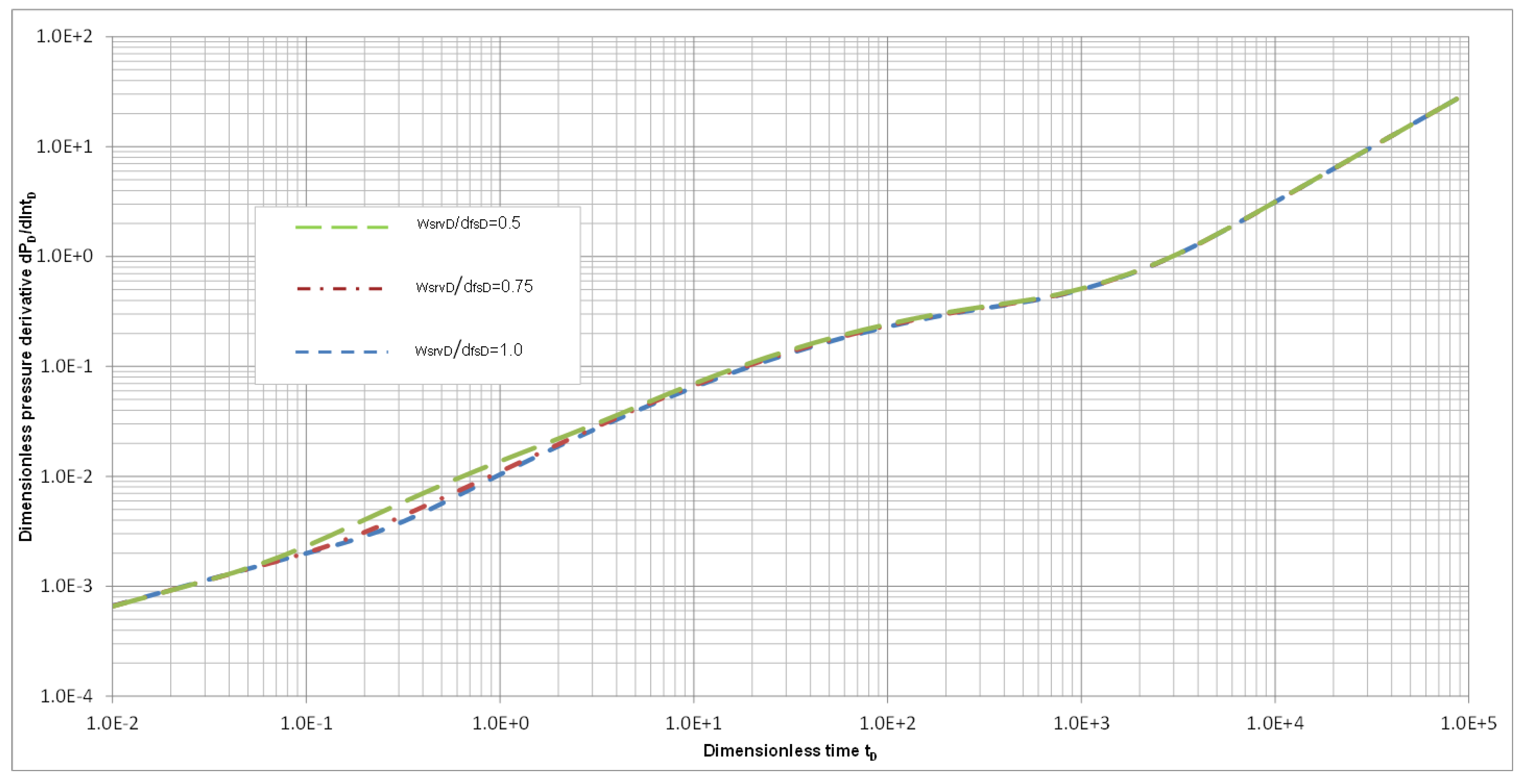
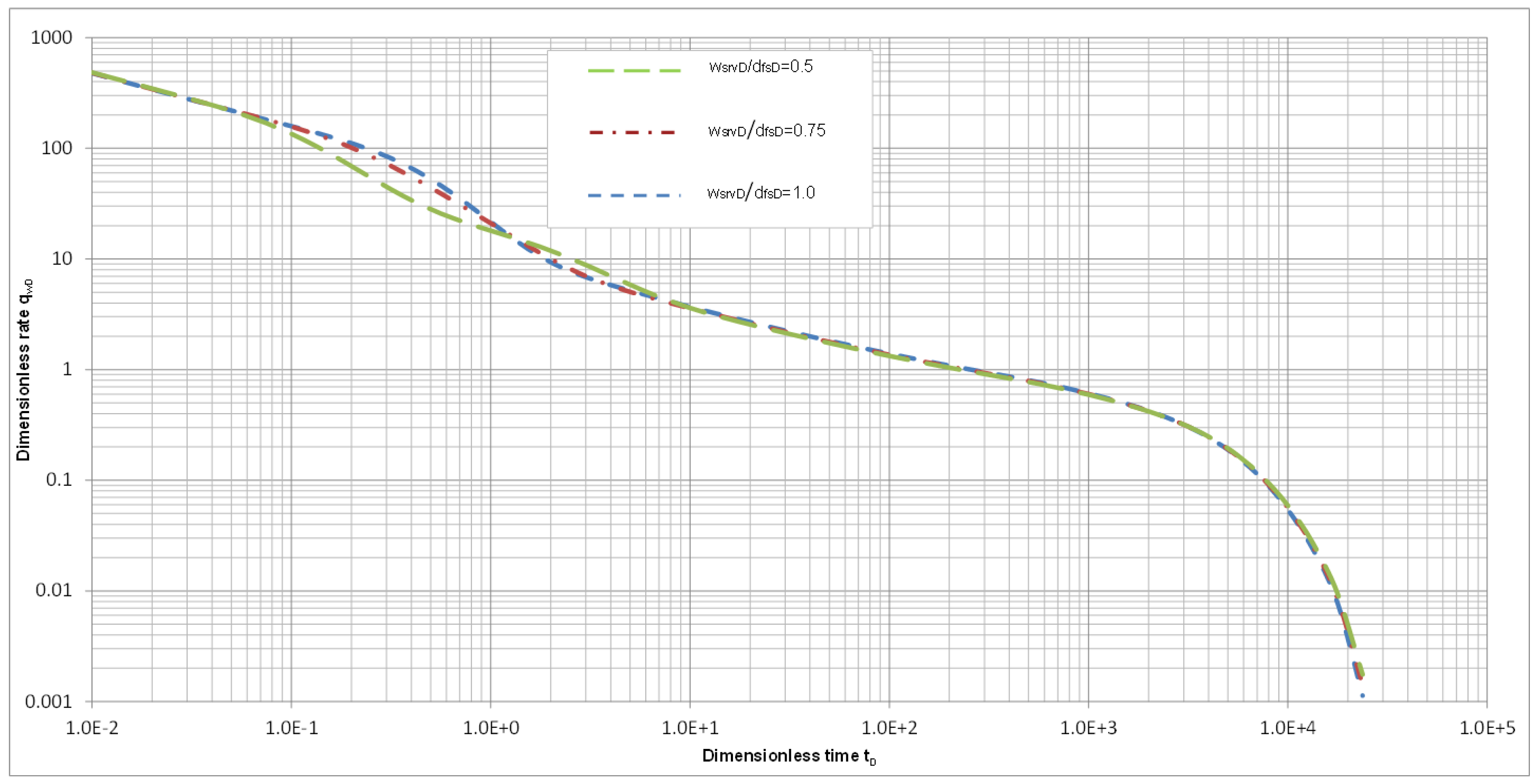
3.3.2. Effect of Local SRV Size
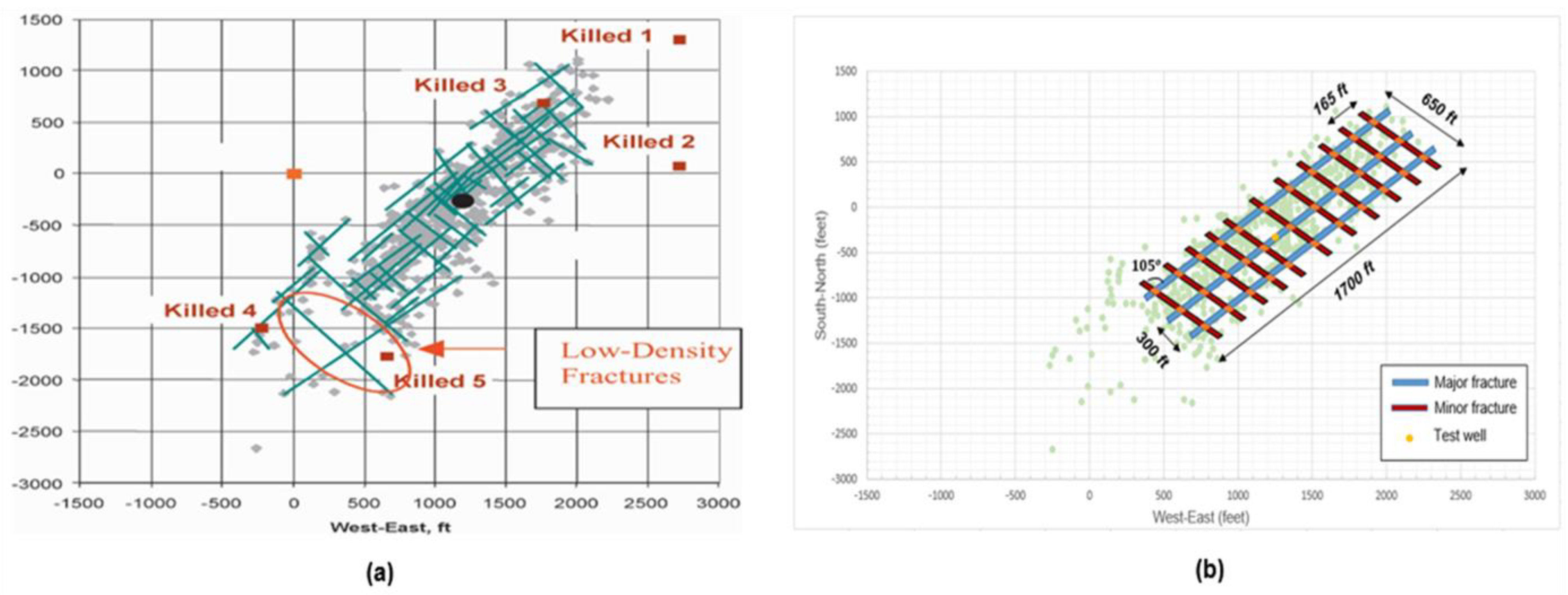
In this scenario, we examine how the width of a local SRV region can affect well behavior when the permeability of the region is enhanced. If the enhanced region accounts for natural fractures around the hydraulic facture, the wider the region, the more natural fractures are indicated to be distributed between hydraulic fractures.
Neither pressure nor rate shows much of a difference among the three curves in Figure 21 and Figure 22. When local SRV regions between hydraulic fractures are connected as W s r v D / d f s D = 1 , the difference in time profile lies mainly between t D = 0.1   to   5 , during which the production rate is roughly as much as 2 times the rate when W s r v D / d f s D = 0.5 . For the case W s r v D / d f s D = 1 , the EFR model becomes a two-region composite reservoir, as local SRV regions between hydraulic fractures are connected. Zhao proposed an SRV model for a fractured, horizontal well to capture the relation between SRV and the original formation. The case of W s r v D / d f s D = 1 in this example represents a similar reservoir model schematic to the model of Zhao [35].
Spatial pressure profiles within the reservoir for such a complex reservoir–well system at a different time t D = 10 ,   100   and   1000 are mapped out and illustrated in Figure 23 with L s r v D / d f s D = 0.5 . The high level of accuracy of the solutions is clearly demonstrated in these profiles.
Theoretical results of various reservoir–well systems from the three examples suggest that the BEM modeling strategy can deal with complex reservoir with multi-scale heterogeneities in an efficient and convenient manner, and the solutions generated possess near analytical accuracy.

4. Field Case Study

This case addresses a complex fracture network using the proposed BEM strategy based on the well-known fracture network interpretation of the microseismic image recorded during hydraulic fracturing by Fisher et al. [36] for the Barnett shale reservoir represented in Figure 24a. The microseismic image is interpreted into a communicated fracture network in the BEM model with the intent of simplifying the problem while capturing the essential features of the fracture network (Figure 24b). The BEM model consists of 3 parallel primary fractures and 11 parallel secondary fractures. Each secondary fracture intersects all 3 primary fractures with an angle of 105°, with the crossing joint section assigned with the properties of either the primary fracture or the secondary fracture. Each primary fracture spans 1700 feet, with 300 feet of spacing between the adjacent primary fractures. The secondary fracture extends 650 feet, with 165 feet spacing. Both the primary fracture and the secondary fracture were assumed to have a fracture width of 0.1 feet. The reservoir is infinite-acting in the model, without the effect of an outer boundary, and the test well is placed in the central portion of the middle primary fracture. Although further detailed modeling with a more complicated fracture network can be performed systematically, it was deemed to be unnecessary at this stage due to the lack of detailed supporting field geology, reservoir, and testing information.
The complexity of this field case and the information provided in the work of Fisher et al. have encouraged general investigation under the given fracture network [36]. The solutions are presented in dimensionless terms, such that the other reservoir properties are not included here. The focus is on the mobility contrasts of the primary and secondary fractures with respect to the reservoir, i.e., the ratios among Mm, Mp, and Ms. We are particularly interested in the effect of the mobility of the fracture crossing section on well performance. Under this context, 6 cases are planned, with details shown in Table 1. The mobility ratio comparison of Mp:Ms:Mm plus the mobility information for the fracture crossing section for the cases based on the simplified fracture network model after Fisher et al. are listed. The computational results using the BEM model constructed are shown in Figure 25 for the dimensionless pressure and Figure 26 for the derivatives of the dimensionless pressure under unit rate conditions. Figure 27 illustrates the dimensionless rate-decline curve under unit pressure-drop conditions.
The first case has the mobility ratio of the primary fracture and the secondary fracture to the original reservoir matrix as 1000 and 100, respectively. The second case has the mobility ratio of the primary fracture and the secondary fracture to the original reservoir matrix as 100 and 10, respectively. The third case sets all fractures and the original reservoir matrix as having the same mobility in simulating a homogeneous reservoir production.
Note that Cases 5 and 6 are essentially the same. Figure 25 and Figure 26 show that the results of these 2 cases exactly overlap each other, which is the standard solution of an infinite acting vertical well in a homogeneous reservoir mathematically described by P D = 1 2 E i ( r D 4 t D ) . This, to a great degree, validates the solution accuracy of the BEM model constructed in this work.
For Case 1, when the mobility of the fracture network is large, with the fracture crossing section having primary fracture mobility (Mp), bi-linear flow with a pressure derivative showing 1/4 slope is clearly seen in the very beginning, followed by linear flow with a pressure derivative showing 1/2 slope. Following the linear flow, the pressure derivative slope becomes slightly greater than 1/2, accounting for the influence of effective SRV surrounding the fracture network area. Finally, the pressure derivative approaches 0.5 as normal. For Case 2, when the mobility of the fracture network is not so dramatic with the fracture crossing section having Mp, the pressure derivative behavior becomes more complicated than expected and requires further investigation in a future research effort. As the fracture crossing section with Ms applies, shown as the dashed curves in Figure 25 and Figure 26, it clearly exhibits that the complexity of the well response increased. In general, because Ms < Mp, the flow process becomes more challenging for Cases 4 and 5, resulting in less productive qD(tD) curves, as shown in Figure 27. This can be applied in Barnett shale field production data analysis as a preliminary study before incorporating shale gas desorption process in analysis. These outcomes confirm our speculation at the time of designing the cases to be studied that the properties of the fracture crossing section do play an important role as far as accurately evaluating the fracture network contribution to fluid flow is concerned.
General speaking, the large difference among those derivative curves offers a great opportunity to characterize the fracture network and identify the conductive nature of both the primary and secondary fractures. The results provide valuable information that needs to be studied further. Due to the limitation of field information provided in the work of Fisher et al. [36], exemplifying a general solution coverage in Figure 25, Figure 26 and Figure 27 can be regarded as satisfactory.

5. Conclusions

Based on the study, the following conclusions can be drawn:
A general computing framework has been developed using the BEM strategy to address the need for describing the complicated geological features of actual heterogeneous reservoirs. This strategy solves the transient behaviors of a complex heterogeneous reservoir with two unique features; one is that the regionalization of each irregular simulation domain is based on the need for describing the geologically heterogeneous feature of local regions of interest, and the other is that the BEM method can handle the complicated boundary shapes and is able to generate solutions with near analytical accuracy.
By applying BEM, boundary discretization and approximation are only made on the boundary enclosing the specific flow domain with uniform fluid/rock properties. No further gridding or sub-partition inside the domain is necessary to further improve solution accuracy. Problems of grid orientation, grid size, and other numerical challenges encountered in other simulation methods are largely eliminated. In addition, numerical solutions are pursued in the Laplace domain by taking numerical Laplace transforms, and thereby, the simulation scheme is freed from time step restriction. This strategy helps reduce computational costs and models the physics of fluid flow in heterogeneous reservoirs more efficiently and reliably.
An important observation from the simplified fracture network modeling after a well-known field case study confirmed that, not only the exemplified complicated fracture network can be accurately modeled semi-analytically, but also the properties of the fracture crossing section do play an important role as far as the fracture network contribution to fluid flow is to be evaluated more reliably with confidence. The exemplification of the empirical, complicated fracture network modeling indicates a significant technical advancement.
This BEM-based technology has great capability and is advantageous in modeling complex geological features of heterogeneous reservoirs, such as naturally fractured reservoirs, fluvial reservoirs with wandering sandbars and channels, fully compartmentalized reservoirs, isolated fracture networks, and reservoirs produced by multi-stage fractured horizontal wells with near-fracture heterogeneities, etc. The simulation technology in this technical domain can be significantly expanded, based on the new realization and understanding achieved from this work. Currently, only single-phase flow is studied in this work. Future study will focus on multiphase flow and phase-behavior integration under complicated scenarios using BEM strategy.
Aiming at reducing the technical gap between reservoir engineering practice and simulation capacity, the work conducted in this research demonstrates the significance of adapting the BEM strategy in next-generation reservoir simulation practice due to its flexibility in handling reservoir heterogeneity, analytical solution accuracy, and high computing efficiency.
What has been achieved in this work can be categorized as: 1. Providing a general theoretical framework in detail, with proven solutions for real field cases and potential scenarios, to handle the complexity in reservoir–well system modeling; 2. Showcasing the accurate and reliable modeling of reservoir heterogeneity and complex natural fracture network systems semi-analytically; and 3. Demonstrating and pointing out the future of next-generation reservoir simulation by adapting BEM strategy, mainly due to its identified flexibility, powerfulness, and accuracy in complicated reservoir heterogeneity simulation.

Author Contributions

Conceptualization, C.S., G.Z. and Y.-C.J.; methodology, C.S., G.Z. and Y.-C.J.; software, C.S. and G.Z.; validation, C.S. and G.Z.; formal analysis, C.S. and W.Y.; investigation, C.S. and W.Y.; resources, G.Z.; data curation, C.S. and G.Z.; writing—original draft preparation, C.S.; writing—review and editing, C.S., W.Y., Y.-C.J. and G.Z.; visualization, C.S. and W.Y.; supervision, Y.-C.J. and G.Z.; project administration, G.Z.; funding acquisition, G.Z. and Y.-C.J. All authors have read and agreed to the published version of the manuscript.

Funding

This research was partially funded by the Petroleum Technology Research Centre (PTRC), NO. 24860, the Faculty of Graduate Studies and Research (FGSR), and the Faculty of Engineering and Applied Science of the University of Regina.

Data Availability Statement

Not applicable.

Acknowledgments

The primary portion of this work was completed during the Ph.D. program of the first author. Our sincere thanks go to Kei Lo for dedicated proofreading.

Conflicts of Interest

The authors declare no conflict of interest.

Nomenclature

c t =total compressibility of reservoir, 1/Pa
C s =storativity, 1/Pa
C R =diffusivity, m2/s
G =free-space Green’s function
h =reservoir vertical thickness, m
k =permeability, m2
L=length, m
L f =fracture half-length, m
M =mobility, m 2 / Pa · s
n =the outward-pointing normal on a boundary element
N =discretized number of boundary element for a flow domain
N e =discretized number of boundary element for a reservoir outer boundary directly surrounding the outer region
N w =number of sources/sinks in a flow domain
p =pressure, Pa
Δ p = p p i ,   Pa
q =rate of source/sink, m 3 / s
q w =producing rate of well, m 3 / s
s =Laplace variable
t =time, s
x =horizontal coordinate, m
x =x coordinate of the source/sink point, m
y =horizontal coordinate, m
y =y coordinate of the source/sink point, m
ξ =local coordinate for boundary element, m
ζ =local coordinate for boundary element, m
η =reservoir diffusivity, m 2 / s
μ =fluid viscosity, Pa · s
τ =time variable, s
ϕ =porosity of the reservoir, fraction
δ=the Dirac delta function
θ =included angle between two boundary elements, or the term defined in Equation (3)
Θ ^ =the function term defined in Equation (A23)
Θ ˜ =the function term defined in Equation (A24)
Ω =locally homogeneous domain
Γ =enclosed boundary for domain Ω
Γ o u t e r =reservoir outer boundary
k =the k-th boundary element
Subscripts
e =boundary related term
i =initial
j =the j-th flow domain
k =the k-th boundary element
m=reservoir matrix
p=primary fractures
ref=reference system
s=secondary fractures
D =dimensionless term
SRV=stimulated reservoir volume

Appendix A. Dimensionless Terms Defined

Dimensionless pressure and dimensionless time are defined in terms of reference rock and fluid properties:
p D = 2 π k r e f h ( q μ ) r e f Δ p ,
t D = k r e f t ( ϕ μ c t ) r e f l 2 ,
where the reference properties of rock/fluid are based on the referenced reservoir system, and the characteristic length, l , can be randomly defined.
Dimensionless rate of source/sink is defined under a constant reference rate, q r e f
q D = q q r e f .  
Dimensionless x- and y-coordinates are defined as:
x D = x l ,  
y D = y l .  
Dimensionless mobility ratio of each region is based on the reference mobility:
M j M r e f = ( k μ ) j ( k μ ) r e f , j [ 1 , 8 ] .
Dimensionless storativity of each region is also based on the reference storativity:
C s j C s r e f = ( ϕ c t ) j ( ϕ c t ) r e f , j [ 1 , 8 ] .
Dimensionless diffusivity ratio is:
C R j C R r e f = ( M C s ) j ( M C s ) r e f , j [ 1 , 8 ] .
Dimensionless well-rate under constant bottom flowing pressure is defined as:
q w D = q w μ r e f 2 π k r e f h Δ p w f .

Appendix B. Pressure Solution Derivation of the Outer Region

It is schematically shown in Figure A1 that Region 8 is a multiply connected domain with complex internal interfaces and with an outer no-flow boundary that directly surrounds this region. From the perspective of Region 8, the other 7 regions behave as if they were “holes” physically extracted out of the original reservoir with their untamed pressures and pressure gradients existing along the boundaries exerted with this region.
Figure A1. The reservoir from the perspective of Region 8.
Minerals 12 00663 g0a1
The following step is to fictitiously divide Region 8 into several simple domains by introducing necessary auxiliary curves. It is shown in Figure A2 that, by introducing auxiliary lines AB and CD, as well as MN and PQ, with a negligible spanning distance as ε 0 , Region 8 becomes a simply connected domain with an interface/boundary expressed as Γ 8 , which is:
Γ 8 = Γ A B + ( Γ o u t e r Γ 2 , o u t e r ) + ( Γ 2 Γ 2 , o u t e r ) + Γ M N + Γ N R S P + Γ P Q + Γ C D + Γ 1 .
Figure A2. Region 8 fictitiously divided into a simply connected region.
Minerals 12 00663 g0a2
With the boundary given by Equation (A10), pressure within this region, similar to Equation (2), now can be written as:
θ 8 2 π p D 8 ( x D , y D , t D ) = 0 t D [ Γ A B ϑ 8 d Γ + Γ o u t e r Γ 2 , o u t e r ϑ 8 d Γ + Γ 2 Γ 2 , o u t e r ϑ 2 d Γ + Γ M N ϑ 8 d Γ + Γ N R S P ϑ i d Γ + Γ P Q ϑ 8 d Γ + Γ C D ϑ 8 d Γ + Γ 1 ϑ 1 d Γ + k = 1 N w 8 q D 8 , k G 8 ]   d τ ,
where θ 8 has the same definition as:
θ 8 = 2 π i f   ( x , y ) Ω 8 θ 8 = θ 8 i f   ( x , y ) Γ 8 ,
and
ϑ j = M 8 M r e f C s r e f C s 8 ( G 8 p D j n p D j G 8 n ) j [ 1 , 8 ] ,
and i { 3 ,   5 ,   6 ,   7 } , one may referring to Figure 1 for the details of the regions defined. The subscript “i” in Equation (A11) represents the regions that connect to Region 8 with the interface that is a portion of the cross-like Γ N R S P .
The pressure expression in Equation (A11) can be further simplified because of the fact that the sum of the four-line integrals—integration along line AB, CD, MN, and PQ—practically equals zero. For Region 8, the outward-pointing normals on lines AB and CD, and on MN and PQ, are opposite of each other. Since the distance ε between the lines is assumed to be negligible, the fluid leaving AB (CD) is entering CD (AB), so that the rate (pressure gradient) must be the same, which makes
A B ϑ 8 d Γ = C D ϑ 8 d Γ ,  
M N ϑ 8 d Γ = P Q ϑ 8 d Γ .  
Assuming that the pressure gradient, from the perspective of each of the seven regions, on the interfaces connected to Region 8 hydraulically, is pointing consistently to the outward normal direction, the p n or G n on the same boundary interface is then pointing to the inward normal direction, from the perspective of Region 8. A “negative” sign, therefore, should be added to curve integrals integrated along ( Γ 2 Γ 2 , o u t e r ) , Γ 1 , and Γ N R S P for Equation (A11). Now, pressure solution within Region 8 becomes
θ 8 2 π p D 8 ( x D , y D , t D ) = 0 t D [ Γ o u t e r Γ 2 , o u t e r ϑ 8 d Γ Γ 2 Γ 2 , o u t e r ϑ 2 d Γ Γ N R S P ϑ i d Γ Γ 1 ϑ 1 d Γ + k = 1 N w 8 q D 8 , k G 8 ] d τ .

Appendix C. Pressure Solution in Discrete Form

As shown in Figure A3, Γ j ( j [ 1 , 7 ] ) is respectively discretized into N j boundary elements, and ( Γ o u t e r Γ 2 , o u t e r ) is discretized into N e boundary elements. Applying the discretization to Equations (2) and (5), the pressure solution within each region can be expressed in its discrete form consisting of the integrals of all the boundary elements discretized along its corresponding boundary.
Figure A3. Scheme of boundary discretization.
Minerals 12 00663 g0a3

Pressure in Region 1 to 7 in Discrete Form

The contour integral of Equation (2) is now written in discrete form, which gives
θ j k 2 π p D j ( x D , y D , t D ) = 0 t D { M j M r e f C s r e f C s j [ k = 1 N j p D j k n Γ j k G j d Γ k = 1 N j p D j k Γ j k G j n d Γ ] + k = 1 N w j q D j , k G j } d τ ,
with
θ j k = 2 π   i f   ( x , y ) Ω j θ j k = π   i f   ( x , y ) Γ j j [ 1 , 7 ] ;   k [ 1 , N j ] .
In Equation (A17), the superscript “k” for pressure stands for the k-th boundary element of Γ j . As spatial pressure and pressure gradient along each element are approximated as being constant, we have them on the k-th boundary element of Γ j as
p D j ( x D , y D , t D ) p D j k ( t D ) ,   f o r   ( x D , y D ) Γ j k ,
p D j n ( x D , y D , t D ) p D j k n ( t D ) ,   f o r   ( x D , y D ) Γ j k .
The evaluation of line integrals, which are free-space Green’s functions and their derivatives integrated along each boundary element, is tedious and inconvenient as the integration path spans two dimensions and the slope of each element is different. To avoid this difficulty and also help attain consistent and high computing accuracy, a general, local coordinate system is defined, based on the element on which the spatial integration is performed.
Figure A4 illustrates the global Cartesian coordinate system, x O y , and the local Cartesian coordinate system for the k-th element of Γ j , ξ j k O j k ζ j k . The locations of the starting node and ending node of the k-th element are marked as ( x n o d , j k , y n o d , j k ) and ( x n o d , j k + 1 , y n o d , j k + 1 ) in the global coordinate system. The local coordinate has the element to lie on its ξ j k -axis, has the included angle j k between x -axis and ξ j k -axis, and has its origin O j k in the global coordinate system at ( g , h ) . From the perspective of this local coordinate system, any point with x- and y-coordinates in the global coordinate system now has ξ j k - and ζ j k -coordinates as
ξ j k = ( x g ) cos j k + ( y h ) sin j k ,
ζ j k = ( y h ) cos j k ( x g ) sin j k ,
with the defined local coordinate system and Equation (A21) and Equation (A22), the line integrals in Equation (A17) now can be evaluated analytically, which is
Θ ^ j k ( x D , y D , x D , y D , t D , τ D ) = Γ j k G j d Γ = Γ j k 1 4 π C R j C R r e f ( t τ ) D exp [ ( x x ) D 2 + ( y y ) D 2 4 C R j C R r e f ( t τ ) D ] d Γ = ξ n o d , j k ξ n o d , j k + 1 1 4 π C R j C R r e f ( t τ ) D exp [ ( ξ j k ξ ) D 2 + ( ζ j k 0 ) D 2 4 C R j C R r e f ( t τ ) D ] d ξ = 1 4 C R j C R r e f π ( t τ ) D · { erf [ ( ξ n o d , j k + 1 ξ j k ) D 2 C R j C R r e f ( t τ ) D ] erf [ ( ξ n o d , j k ξ j k ) D 2 C R j C R r e f ( t τ ) D ] } · exp [ ( ζ j k ) D 2 4 C R j C R r e f ( t τ ) D ]
Figure A4. Local coordinate system defined for k-th element on Γ j .
Minerals 12 00663 g0a4
By applying the same procedure, the other integral, which is the derivative of a free-space Green’s function integrated along the element, can be obtained, and it is given as:
Θ ˜ j k ( x D , y D , x D , y D , t D , τ D ) = Γ j k G j n d Γ = ζ j k 2 C R j C R r e f ( t τ ) D 1 4 C R j C R r e f π ( t τ ) D { erf [ ( ξ n o d , j k + 1 ξ j k ) D 2 C R j C R r e f ( t τ ) D ] erf [ ( ξ n o d , j k ξ j k ) D 2 C R j C R r e f ( t τ ) D ] } erf [ ( ξ n o d , j k ξ j k ) D 2 C R j C R r e f ( t τ ) D ] .
with the analytical evaluation of line integrals; the pressure solution within Region j ( j ∈ [1,7]) can be expressed as:
θ j k 2 π p D j ( x D , y D , t D ) = 0 t D { M j M r e f C s r e f C s j [ k = 1 N j p D j k ζ j k Θ ^ j k k = 1 N j p D j k Θ ˜ j k ] + k = 1 N w j q D j , k G j } d τ ,

Pressure in Region 8 in Discrete Form

Using similar procedures as those we have taken for the pressure in the first seven regions, the pressure solution within Region 8 by Equation (5) can also be expressed in discrete form, which yields:
θ 8 k 2 π p D 8 ( x D , y D , t D ) = M 8 M r e f C s r e f C s 8 { 0 t D [ k = 1 N e p D 8 k ζ 8 k Θ ^ 8 k k = 1 N e p D 8 k Θ ˜ 8 k ] d τ 0 t D [ k = 1 N 2 , 8 p D 2 k ζ 2 k Θ ^ 8 k k = 1 N 2 , 8 p D 2 k Θ ˜ 8 k ] d τ 0 t D [ k = 1 N N R S P p D i k ζ i k Θ ^ 8 k k = 1 N N R S P p D i k Θ ˜ 8 k ] d τ 0 t D [ k = 1 N 1 p D 1 k ζ 1 k Θ ^ 8 k k = 1 N 1 p D 1 k Θ ˜ 8 k ] d τ } + 0 t D k = 1 N w 8 q D 8 , k G 8   d τ
where,
θ 8 k = 2 π   i f   ( x , y ) Ω 8   θ 8 k = π   i f   ( x , y ) Γ 8   k [ 1 , N e + N 2 , 8 + N N R S P + N 1 ] .
On the right hand side of Equation (A26), the first term accounts for line integrals along ( Γ o u t e r Γ 2 , o u t e r ) , the second along ( Γ 2 Γ 2 , o u t e r ) , the third along the boundary of the cross-like Γ N R S P , and the fourth along Γ 1 . The total number of boundary elements for ( Γ 2 Γ 2 , o u t e r ) is denoted by N 2 , 8 , and for Γ N R S P is denoted by N N R S P as N N R S P = N 3 + N 5 + N 6 + N 7 N 4 .

References

  1. Carslaw, H.S.; Jaeger, J.C. Conduction of Heat in Solids, 2nd ed.; Oxford at the Clarendon Press: Oxford, UK, 1959. [Google Scholar]
  2. Gringarten, A.C.; Ramey, H.J., Jr. The Use of Source and Green’s Functions in Solving Unsteady-Flow Problems in Reservoirs. Soc. Pet. Eng. J. 1973, 13, 285–296. [Google Scholar] [CrossRef]
  3. Gringarten, A.C.; Ramey, H.J., Jr.; Raghavan, R. Unsteady-State Pressure Distributions Created by a Well With a Single Infinite-Conductivity Vertical Fracture. Soc. Pet. Eng. J. 1974, 14, 347–360. [Google Scholar] [CrossRef] [Green Version]
  4. Ozkan, E.; Raghavan, R. New Solutions for Well-Test-Analysis Problems: Part 1—Analytical Considerations. SPE Form. Eval. 1991, 6, 359–368. [Google Scholar] [CrossRef] [Green Version]
  5. Ozkan, E.; Raghavan, R. New Solutions for Well-Test-Analysis Problems: Part 2—Computational Considerations and Applications. SPE Form. Eval. 1991, 6, 369–378. [Google Scholar] [CrossRef]
  6. Ramey, H.J. Approximate Solutions For Unsteady LiquidFlow In Composite Reservoirs. J. Can. Pet. Technol. 1970, 9, 32–37. [Google Scholar] [CrossRef]
  7. Kuchuk, F.J.; Habashy, T. Pressure Behavior of Laterally Composite Reservoirs. SPE Form. Eval. 1997, 12, 47–56. [Google Scholar] [CrossRef]
  8. Basquet, R.; Alabert, F.G.; Caltagirone, J.P.; Batsale, J.C. A Semianalytical Approach for Productivity Evaluation of Complex Wells in Multilayered Reservoirs. SPE Reserv. Eval. Eng. 1999, 2, 503–513. [Google Scholar] [CrossRef]
  9. Medeiros, F.; Ozkan, E.; Kazemi, H. A Semianalytical Approach To Model Pressure Transients in Heterogeneous Reservoirs. SPE Reserv. Eval. Eng. 2010, 13, 341–358. [Google Scholar] [CrossRef]
  10. Zhao, G.; Thompson, L.G. Transient Pressure Analysis of Bounded Communicating Reservoirs. In Proceedings of the SPE Rocky Mountain Petroleum Technology Conference, Keystone, CO, USA, 21–23 May 2001. [Google Scholar] [CrossRef]
  11. Zhao, G.; Thompson, L.G. Semianalytical Modeling of Complex-Geometry Reservoirs. SPE Reserv. Eval. Eng. 2002, 5, 437–446. [Google Scholar] [CrossRef]
  12. Zhao, G.; Thompson, L.G. Transient Pressure Response of Fluvial Reservoir with Branching Channel and Splay. In Proceedings of the 2001 SPE Annual Technical Conference and Exhibition, New Orleans, LO, USA, 30 September–3 October 2001. [Google Scholar] [CrossRef]
  13. Zhao, G.; Thompson, L.G. Well Testing Analysis in Heterogeneous Reservoir Using Semi-Analytical Method. In Proceedings of the 55th Annual Technical Meeting, Canadian International Petroleum Conference (CIPC), Petroleum Society Canadian Institute of Mining, Metallurgy & Petroleum, Calgary Stampede Roundup Centre, Calgary, AB, Canada, 8–10 June 2004. [Google Scholar]
  14. Zhao, G. Reservoir Modeling Method. U.S. Patent 8,275,593, 25 September 2012. [Google Scholar]
  15. Kikani, J.; Horne, R.N. Pressure-Transient Analysis of Arbitrarily Shaped Reservoirs With the Boundary-Element Method. SPE Form. Eval. 1992, 7, 53–60. [Google Scholar] [CrossRef]
  16. Xiao, L.; Zhao, G.; Qing, H. A Compatible Boundary Element Approach with Geologic Modeling Techniques to Model Transient Fluid Flow in Heterogeneous Systems. J. Pet. Sci. Eng. 2017, 151, 318–329. [Google Scholar] [CrossRef]
  17. Wu, M.; Ding, M.; Yao, J.; Li, C.; Huang, Z.; Xu, S. Production-Performance Analysis of Composite Shale-Gas Reservoirs by the Boundary-Element Method. SPE Reserv. Eval. Eng. 2018, 22, 238–252. [Google Scholar] [CrossRef] [Green Version]
  18. Lennon, G.P.; Liu, P.L.-F.; Liggett, J.A. Boundary Integral Solutions to Three-Dimensional Unconfined Darcy’s Flow. Water Resour. Res. 1980, 16, 651–658. [Google Scholar] [CrossRef]
  19. Lafe, O.E.; Liggett, J.A.; Liu, P.L.-F. BEIM Solutions to Combinations of Leaky, Layered, Confined, Unconfined, Nonisotropic Aquifers. Water Resour. Res 1981, 17, 1431–1444. [Google Scholar] [CrossRef]
  20. Azevedo, J.P.S.; Wrobel, L.C. Non-Linear Heat Conduction in Composite Bodies: A Boundary Element Formulation. Int. J. Numer. Methods Eng. 1988, 26, 19–38. [Google Scholar] [CrossRef]
  21. Bialecki, R.; Kuhn, G. Boundary Solution of Heat Conduction Problems in Multizone Bodies of Non-Linear Materials. Int. J. Numer. Methods Eng. 1993, 36, 799–809. [Google Scholar] [CrossRef]
  22. Kikani, J.; Horne, R.N. Modeling Pressure-Transient Behavior of Sectionally Homogeneous Reservoirs by the Boundary-Element Method. SPE Form. Eval. 1993, 8, 145–152. [Google Scholar] [CrossRef]
  23. Layne, M.A.; Numbere, D.T.; Koederitz, L.F. Future Performance Prediction for Water Drive Gas Reservoirs. In Proceedings of the SPE Annual Technical Conference and Exhibition, Houston, TX, USA, 3 October 1993. [Google Scholar] [CrossRef]
  24. Pecher, R.; Stanislav, J.F. Boundary Element Techniques in Petroleum Reservoir Simulation. J. Pet. Sci. Eng. 1997, 17, 353–366. [Google Scholar] [CrossRef]
  25. Xiao, L.; Zhao, G. Estimation of CHOPS Wormhole Coverage From Rate/Time Flow Behaviors. SPE Reserv. Eval. Eng. 2017, 20, 957–973. [Google Scholar] [CrossRef]
  26. Wu, Y.; Cheng, L.; Fang, S.; Huang, S.; Jia, P. A Green Element Method-Based Discrete Fracture Model for Simulation of the Transient Flow in Heterogeneous Fractured Porous Media. Adv. Water Resour. 2020, 136, 103489. [Google Scholar] [CrossRef]
  27. Su, C. Semi-Analytical Modeling of Fluid Flow in and Formation Evaluation of Unconventional Reservoir Using Boundary Integration Strategies. Dissertation, University of Regina, Saskatchewan, SK, Canada, 2018. [Google Scholar]
  28. Onur, M.; Reynolds, A.C. Numerical Laplace Transformation of Sampled Data for Well-Test Analysis. SPE Reserv. Eval. Eng. 1998, 1, 268–277. [Google Scholar] [CrossRef]
  29. Stehfest, H. Numerical Inversion of Laplace Transforms. Commun. ACM 1970, 13, 47. [Google Scholar] [CrossRef]
  30. Karimi-Fard, M.; Durlofsky, L.J. A General Gridding, Discretization, and Coarsening Methodology for Modeling Flow in Porous Formations With Discrete Geological Features. Adv. Water Resour. 2016, 96, 354–372. [Google Scholar] [CrossRef]
  31. Xu, Y.; Cavalcante Filho, J.S.; Yu, W.; Sepehrnoori, K. Discrete-Fracture Modeling of Complex Hydraulic-Fracture Geometries in Reservoir Simulators. SPE Reserv. Eval. Eng. 2016, 20, 403–422. [Google Scholar] [CrossRef]
  32. Zhao, G. Modeling Complex Natural Fracture Network in Heterogeneous Tight Formations Using Semi-Analytical Strategy. In Proceedings of the SPE Unconventional Resources Conference, Calgary, AB, Canada, 5 November 2013. [Google Scholar] [CrossRef]
  33. Stalgorova, E.; Mattar, L. Analytical Model for Unconventional Multifractured Composite Systems. SPE Reserv. Eval. Eng. 2013, 16, 246–256. [Google Scholar] [CrossRef]
  34. Chen, C.; Raghavan, R. On Some Characteristic Features of Fractured-Horizontal Wells and Conclusions Drawn Thereof. SPE Reserv. Eval. Eng. 2013, 16, 19–28. [Google Scholar] [CrossRef]
  35. Zhao, G. A Simplified Engineering Model Integrated Stimulated Reservoir Volume (SRV) and Tight Formation Characterization With Multistage Fractured Horizontal Wells. In Proceedings of the SPE Canadian Unconventional Resources Conference, Calgary, AB, Canada, 30 October 2012. [Google Scholar] [CrossRef]
  36. Fisher, M.K.; Wright, C.A.; Davidson, B.M.; Goodwin, A.K.; Fielder, E.O.; Buckler, W.S.; Steinsberger, N.P. Integrating Fracture Mapping Technologies to Optimize Stimulations in the Barnett Shale. In Proceedings of the SPE Annual Technical Conference and Exhibition, San Antonio, TA, USA, 29 September 2002. [Google Scholar] [CrossRef]
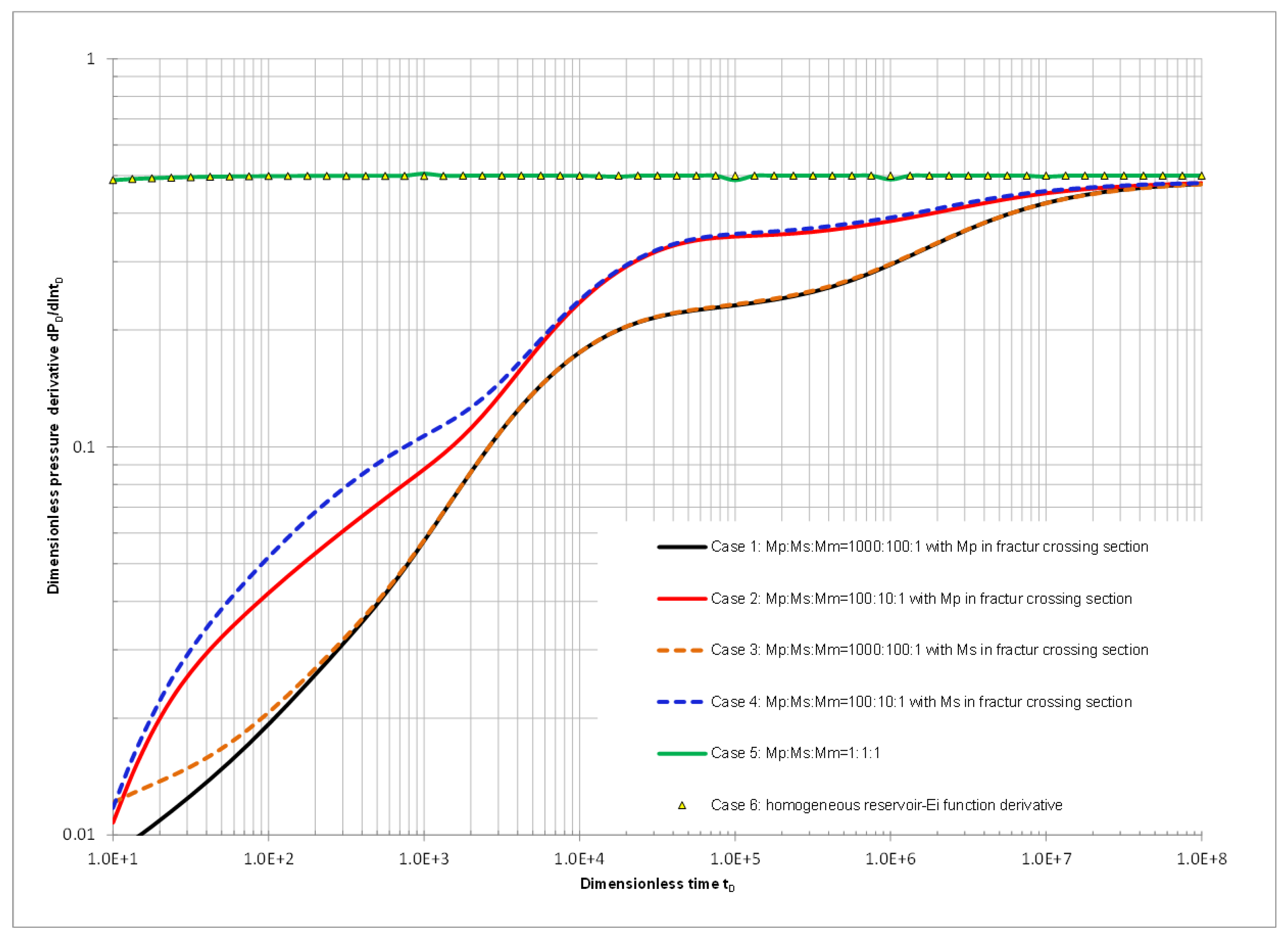
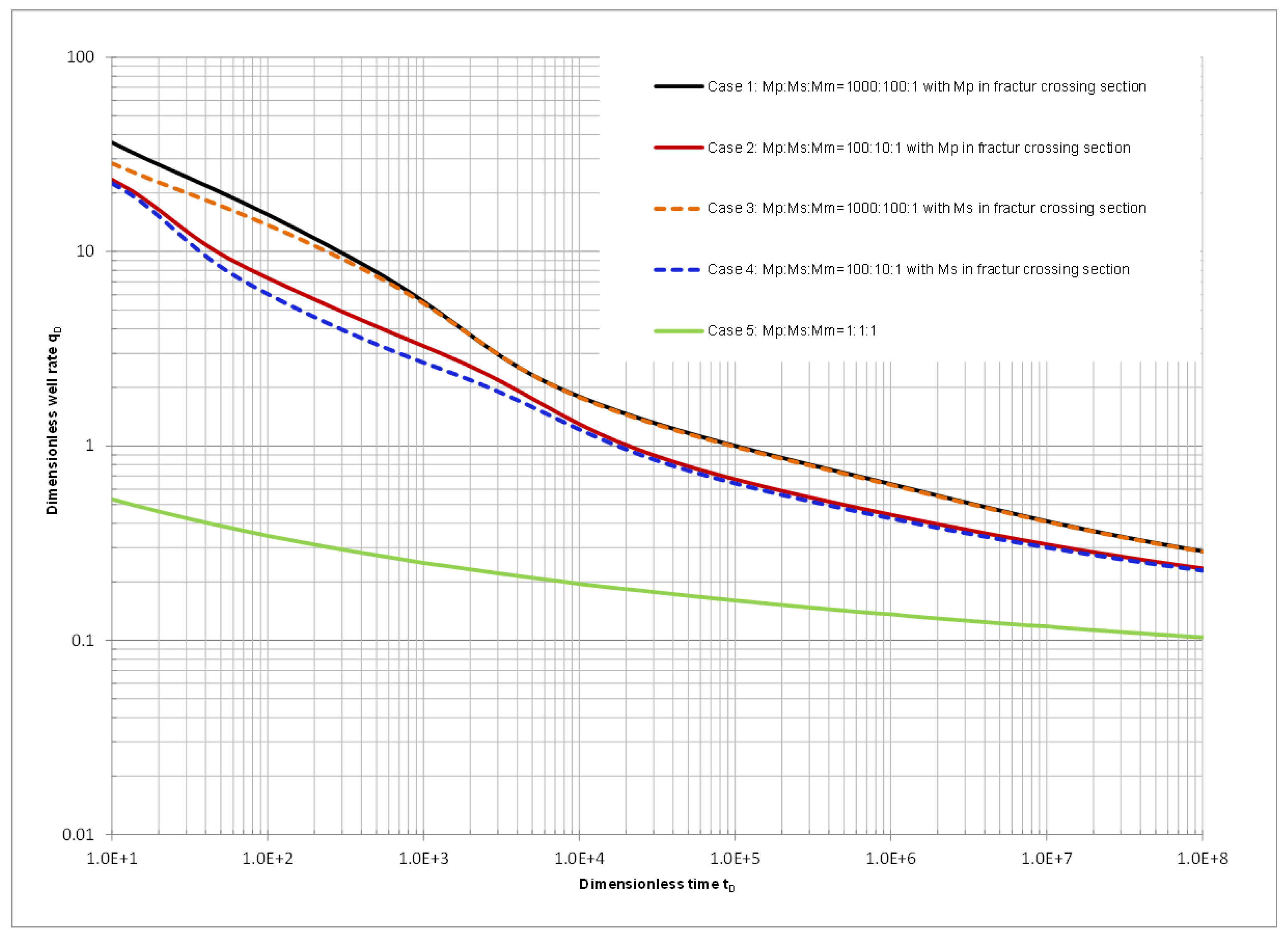
Figure 1. Schematic of the exemplified heterogeneous reservoir with eight regions.
Minerals 12 00663 g001
Figure 2. The perspectives of Regions 1–7 and their integration paths.
Minerals 12 00663 g002
Figure 3. Schematic reservoir with (a) an irregular-gridding system and (b) a rectangular gridding system, X e D = 50 and Y e D = 50 .
Minerals 12 00663 g003
Figure 4. Standard solutions to reservoir schematics in Figure 3a,b under homogeneous reservoir condition, X e D = 50 and Y e D = 50 .
Minerals 12 00663 g004
Figure 5. Comparison between solutions generated by this BEM model and Zhao and Thompson’s SSFM semi-analytical model [10].
Minerals 12 00663 g005
Figure 6. Reservoir with two parallel, natural, fractures bounded by an arbitrarily shaped outer boundary, with the values of all terms shown, W D ,   H D , w f D , and X v D may vary.
Minerals 12 00663 g006
Figure 7. Pressure and its derivative behaviors of a well producing between two sealing faults in comparison to the solutions from Saphir for different 2 L f D H D , with k f r a c / k m a t r i x = 0.0001 , W D = 50 , H D = 50 , w f D = 0.01 , and X v D = 5 .
Minerals 12 00663 g007
Figure 8. Rate behaviors of a well producing between two sealing faults for different 2 L f D H D , with k f r a c / k m a t r i x = 1.0 × 10 4 , W D = 50 , H D = 50 , w f D = 0.01 , and X v D = 5 .
Minerals 12 00663 g008
Figure 9. Pressure and its derivative behaviors of the well with respect to different permeability ratios of natural fracture to formation, W D = 50 , H D = 50 , w f D = 0.01 , 2 L f D = 10 , and X v D = 2 .
Minerals 12 00663 g009
Figure 10. Rate behaviors of the well with respect to different permeability ratios of natural fracture to formation, W D = 50 , H D = 50 , w f D = 0.01 , 2 L f D = 10 , and X v D = 2 .
Minerals 12 00663 g010
Figure 11. Definitions of (a) the LHS and the RHS of the isolated fracture faces and (b) the positive flow direction for flowing flux.
Minerals 12 00663 g011
Figure 12. Flux profiles along the LHS and RHS of the isolated fracture of k f r a c / k m a t r i x = 10 , 000 , with W D = 50 , H D = 50 , w f D = 0.01 , 2 L f D = 10 , and X v D = 2 .
Minerals 12 00663 g012
Figure 13. Flux profiles along the LHS and RHS of the isolated fracture of k f r a c / k m a t r i x = 0.01 , with W D = 50 , H D = 50 , w f D = 0.01 , 2 L f D = 10 , and X v D = 2 .
Minerals 12 00663 g013
Figure 14. Reservoir with isolated, crossing, natural fractures; the variable values of all terms.
Minerals 12 00663 g014
Figure 15. Pressure and its derivative behaviors of a well for different fracture crossing angles under (a)   k f r a c / k m a t r i x = 1.0 × 10 4 and (b)   k f r a c / k m a t r i x = 1.0 × 10 4 , with W D = 50 ,   H D = 50 , L D = 15 ,   2 L f D = 20 , d D = 1 , and w f D = 0.1 .
Minerals 12 00663 g015
Figure 16. Schematic of four wells producing in a fluvial reservoir environment with meandering sandbars under different permeability values, K1 inside sand bar and K2 within fluvial channel.
Minerals 12 00663 g016
Figure 17. Pressure derivatives of the 4 wells under K1/K2=50, CS1/CS2=1.
Minerals 12 00663 g017
Figure 18. MHFHW model with local SRVs of six-stage fractures.
Minerals 12 00663 g018
Figure 19. Pressure and its derivative behaviors of a fractured, horizontal well under a different permeability ratio k 1 / k 2 , with 2 L f D / Y e D = 0.1 , w s r v D / d f s D = 0.5 , X e D = 200 , and Y e D = 100 .
Minerals 12 00663 g019
Figure 20. Rate behaviors of a fractured, horizontal well under a different permeability ratio k 1 / k 2 , with 2 L f D / Y e D = 0.1 , w s r v D / d f s D = 0.5 , X e D = 200 , and Y e D = 100 .
Minerals 12 00663 g020
Figure 21. Pressure response of a fractured, horizontal well under a different ratio of local SRV width and space between fractures as k 1 / k 2 = 20 , 2 L f D / Y e D = 0.1 , X e D = 200 , and Y e D = 100 .
Minerals 12 00663 g021
Figure 22. Rate response of fractured, horizontal well under a different ratio of local SRV width and space between fractures as k 1 / k 2 = 20 , 2 L f D / Y e D = 0.1 , X e D = 200 , and Y e D = 100 .
Minerals 12 00663 g022
Figure 23. Pressure profiles within the entire reservoir at (a)   t D = 10 (b) t D = 100 (c) t D = 1000 with w s r v D / d f s D = 0.5 , 2 L f D / Y e D = 0.2 and k 1 / k 2 = 20 , X e D = 200 , and Y e D = 100 .
Minerals 12 00663 g023
Figure 24. (a) Complex-fracture network interpretation for Barnett shale microseismic image recorded during fracturing (Fisher et al. [36], permission of SPE); (b) a simplified fracture network in the BEM model (after Fisher et al. 2002).
Minerals 12 00663 g024
Figure 25. PD for the six cases based on the simplified fracture network model.
Minerals 12 00663 g025
Figure 26. dPD/d(lntD) responses for the six cases based on the simplified fracture network model.
Minerals 12 00663 g026
Figure 27. qD responses for the six cases based on the simplified fracture network model.
Minerals 12 00663 g027
Table 1. The fracture mobility parameters for the cases based on the simplified fracture network model after Fisher et al. [36].
Mobility Ratio Comparison of
Mp:Ms:Mm
Mobility of
Fracture Crossing Section
Case 11000:100:11000
Case 2100:10:1100
Case 31000:100:1100
Case 4100:10:110
Case 51:1:1homogeneous
Case 6homogeneous reservoirhomogeneous
Publisher’s Note: MDPI stays neutral with regard to jurisdictional claims in published maps and institutional affiliations.

