Abstract
Image segmentation approaches have been utilized to determine the particle size distribution of crushed ores in the past decades. It is not possible to deploy large and high-powered computing equipment due to the complex working environment, so existing algorithms are difficult to apply in practical engineering. This article presents a novel efficient and lightweight framework for ore image segmentation to discern full and independent ores. First, a lightweight backbone is introduced for feature extraction while reducing computational complexity. Then, we propose a compact pyramid network to process the data obtained from the backbone to reduce unnecessary semantic information and computation. Finally, an optimized detection head is proposed to obtain the feature to maintain accuracy. Extensive experimental results demonstrate the effectiveness of our method, which achieves 40 frames per second on our new ore image dataset with a very small model size. Meanwhile, our method maintains a high level of accuracy—67.68% in and 46.73% in —compared with state-of-the-art approaches.
1. Introduction
Ore particle size distribution is a significant parameter for analyzing the effectiveness of operation and status of crushing equipment in the mining process. In the past, ore particle size detection was mainly completed manually. For long-term detection, it requires a large amount of manpower and material resources, and accuracy and efficiency are very low [1]. An increasing number of image processing technologies have been applied to ore particle size detection in recent years. The acquisition of ore images is often done during the ore delivery process. As a result, external physical conditions such as dust and uneven illumination can have a significant impact on ore particle size detection as shown in Figure 1. These external physical conditions present significant challenges to any image segmentation technique.
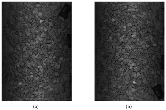
Figure 1.
Image of ore in a real-world working situation. (a) Example 1. (b) Example 2.
Many image processing methods have been proposed in response to these issues. For example, watershed [2,3,4] and FogBank [5] algorithms are often used in region-based segmentation techniques. An effective particle segmentation method [6] was proposed to eliminate the droplets in crystals and particle shadow, but this method is not suitable for ore segmentation with overlapping. The dual-window Otsu threshold [7] is used to determine the threshold value, which reduces the influence of noise, but this method still cannot accurately segment ore images with overlapping and fuzzy boundaries. A watershed transformation approach [8] was permuted to generate superpixels efficiently, but this method is not robust enough and is time-consuming. A regression-based classifier [9] is able to improve the segmentation accuracy of ore particle boundaries by learning ore shape features, but the disadvantage of this method is that the parameters need to be adjusted manually. These technologies have the common disadvantages of slow speed and complicated operation, as well as the inability to deal with ores in complex environments, such as stickiness, dust, and uneven illumination. When traditional methods failed to outperform deep learning approaches in ore segmentation, researchers began to consider deep learning approaches. Ma et al. [1] and Wang et al. [10] proposed two ore image segmentation approaches based on deep learning methods. However, the computing cost of these complicated deep learning methods is prohibitively expensive. In this case, we need approach the problem of ore image segmentation from a different angle.
In recent years, many scholars have been considering the use of deep learning-based approaches to solve real challenges. Deep learning-based methods have higher accuracy and are easier to deploy than the standard approaches mentioned above. A large number of researchers are devoting themselves to applying deep learning-based methods to practical engineering [11]. In comparison to other deep learning-based methods, instance segmentation currently offers the most application potential. More and more instance segmentation algorithms are being used in a variety of scenarios, including medical treatment, road construction, and so on. The two-stage methods (e.g., Mask R-CNN [12]) in instance segmentation have high precision, but slow speed, while the one-stage methods (e.g., YOLACT [13]) have fast speed, but low precision. This demonstrates how the instance segmentation algorithm has significant practical ramifications. However, these methods fail to achieve a balance between speed and precision. In a resource-constrained environment, a lightweight and high accuracy framework is required to meet actual needs, such as real-time speed and small model size. It is well known that the computational costs of deep learning-based algorithms are primarily concentrated in the backbone, neck, and detection head. Therefore, we improve these three components to obtain higher accuracy and real-time instance segmentation at a low computational cost.
In this paper, we propose a light ore segmentation network (LosNet) for real-time ore image analysis. For feature extraction, we first employ a lightweight backbone to dramatically reduce model size and inference time. Then, we propose a lightweight feature pyramid network (FPN) to reduce unnecessary semantic information and computational costs while improving the accuracy and speed. Finally, we suggest an improved detection head to further maintain accuracy. Experiments on our released ore image datasets reveal that our LosNet outperforms the state-of-the-art methods with small model size and real-time speed. In general, our main contributions are as follows.
- We propose an efficient and lightweight network—LosNet—for instance segmentation of ore images;
- We propose a lightweight FPN and an optimized detection head to reduce the computational complexity of the model while increasing the speed;
- We release a new dataset for ore instance segmentation that contains 5120 images manually annotated with bounding boxes and instance masks;
- Extensive quantitative and qualitative experiments on the new ore images dataset show that our LosNet achieves superior performance in comparison with the state-of-the-arts.
The rest of this article is organized as follows. Section 2 introduces related works about general instance segmentation methods and ore segmentation methods. Section 3 presents our overall framework and three individual modules. To verify the effectiveness of our method, we conducted comprehensive experiments, shown in Section 4. Finally, the full text is summarized in Section 5.
2. Related Work
2.1. Ore Image Segmentation
In the past decades, limited by hardware technology, it was difficult to obtain sharp images, and many algorithms that required too much computer performance could not be adopted. Scholars mainly researched image-based system software and hardware framework, contour detection, reasonable measurement parameters, and size transformation functions.
Recently, with the rapid development of computer hardware and new technologies, image-based, online, and real-time particle size measurement development has made much progress. For example, watershed [2,3,4] and FogBank [5] algorithms are often used in region-based segmentation techniques. However, it is difficult to accurately segment the ore particles with fuzzy edges, uneven illumination, and adhesion degree. Threshold-based methods are the most common parallel region technique, and certain requirements were followed to determine the grayscale threshold. For instance, Lu et al. [6] proposed a particle segmentation method to eliminate droplets in crystals and particle shadow by using the background difference and local threshold method, respectively. However, this method is not suitable for ore segmentation with overlapping. Zhang et al. [7] adopted the dual-window Otsu threshold method to determine the threshold value, which reduces the influence of noise and improves the thresholding performance of uneven lighting images efficiently. However, their method still cannot accurately segment ore images with overlapping and fuzzy boundaries. Malladi et al. [8] permuted a watershed transformation approach to generate superpixels efficiently, but this method is not robust enough and is time-consuming. Based on a multi-level strategy, Yang et al. [14] adopted the marker-based region growing method to carry out image segmentation. Mukherjee et al. [9] utilized a regression-based classifier to learn ore shape features, which improved the segmentation accuracy of ore particle boundary, but the parameters were manually adjusted. Zhang et al. [15] reduced noise and separated touching objects by combining wavelet transform and fuzzy c-means clustering for particle image segmentation. Ma et al. [1] devised a method for accurately segmenting belt ore images based on the deep learning method and image processing technologies. However, because this method requires the employment of several algorithms to analyze different types of ore pictures, the algorithm processing procedure is complex and slow. Wang et al. [10] proposed an improved encoder of U-Net based on Resnet18 to improve ore image segmentation accuracy.
2.2. Two-Stage Instance Segmentation
Two-stage instance segmentation splits the task into two subtasks, object detection and segmentation. He et al. [12] presented a conceptually simple, flexible, and general framework Mask R-CNN for object instance segmentation, which extended Faster R-CNN [16] by adding a branch for predicting an object mask in parallel with the existing branch for bounding box recognition. This approach efficiently detected objects in an image while simultaneously generating a high-quality segmentation mask for each instance. Huang et al. [17] researched how to score instance segmentation masks and proposed the mask scoring R-CNN. The network evaluates the IoU of the projected mask and utilizes it to enhance the prediction scores in mask scoring R-CNN. Chen et al. [18] presented a new cascade architecture for instance segmentation called hybrid task cascade (HTC). It uses a semantic segmentation branch to offer spatial context and intertwines box and mask branches for combined multi-stage processing. Kuo et al. [19] introduced class-dependent shape priors and used them as preliminary estimates to obtain the final detection. Liang et al. [20] introduced a novel instance segmentation algorithm that required a mask for the first stage and used polygon representation. The final prediction was obtained by refining the initial mask with a deforming network. Content-aware reassembly of features (CARAFE) is a ubiquitous, lightweight, and highly effective upsampling operator proposed by Wang et al. [21]. Vu et al. [22] proposed an architecture referred to as the sample consistency network (SCNet) to ensure that the IoU distribution of the samples at training time was close to that at inference time. Rossi et al. [23] proposed a novel RoI extraction layer for two-step architectures. The suggested layer built upon intuition by first pre-processing every single layer, aggregating them together, and then applying attentive techniques as post-processing to eliminate unnecessary (global) data.
2.3. One-Stage Instance Segmentation
These above methods accomplish state-of-the-art accuracy, but they are generally slower than one-stage methods. One-stage methods can be roughly divided into two categories: global area-based and local area-based approaches. Global-area-based methods first generate intermediate and shared feature maps based on the whole image, then assemble the extracted features to form the final masks for each instance. YOLACT is a basic, fully-convolutional model for real-time instance segmentation proposed by Zhou et al. [13], and it is one of the first approaches to attempt real-time instance segmentation. YOLACT splits the instance into two parallel jobs, generates a set of prototype masks, and predicts the mask coefficient of each instance. By efficiently merging instance level information with semantic information with lower-level fine granularity, Chen et al. [24] enhanced mask prediction. Instead of predicting a scalar coefficient for each prototype mask, BlendMask predicts a low-resolution (7 × 7) attention map to blend the bounding box of the mask. A single shot and anchor-free instance segmentation approach was presented by Wang et al. [25]. The mask prediction was separated into two important modules: the local form branch, which effectively separates various instances, and the global saliency branch, which achieves pixel-by-pixel segmentation. Tian et al. [26] proposed a simple, yet effective instance segmentation framework, termed CondInst, which went one step further and completely eliminated any dependence on bounding boxes. It does not assemble the cropped prototype mask, but borrows the idea of dynamic filters and predicts the parameters of the lightweight fully convolution network (FCN) header. Wang et al. [27] introduced SOLOv2, which improved the mask detection effect and operation efficiency by adding mask learning and mask non-maximum suppression (NMS) to the elegant and concise design of SOLO [28]. Tian et al. [29] proposed a high-performance method that can achieve mask-level instance segmentation, using only bounding box annotations for training.
3. Approach
In this section, we first introduce the overall framework. Then, we show our proposed lightweight FPN and optimized detection head. Finally, we describe the loss function used in the framework.
3.1. Overall Framework
As discussed before, hardware resources are restricted in the wild. As a result, the instance segmentation model requires a low computational cost. A significant quantity of the computation frequently occurs in the backbone, neck, and detection head. For ore images, the complicated network obtains a large amount of meaningless data, causing the model to grow larger and operate slower. We present real-time instance segmentation for ore images, which consists primarily of a lightweight backbone, a lightweight FPN, and an optimized detection head.
We employ the lightweight backbone MobileNetV3-small [30] to reduce computational costs. In Figure 2, the backbone can generate feature maps across different scales. High-level feature maps provide more semantic information, whereas low-level feature maps have more resolution. The features of different scales are input into the FPN [31]. The rich semantic information of the upper-layer feature maps is conveyed to the lower-layer high-resolution feature maps for fusion. After that, the fusion feature maps are input into the detection head. The detection head has the following output heads. The classification head predicts the class of the instance associated with the location. The regression head can regress the four distances of the prediction bounding boxes. The centerness head is used to suppress the low-quality detected bounding boxes. The controller head, which has the same architecture as the abovementioned classification head, is used to predict the parameters of the mask head for the instance at the location. The P3, P4, and P5 layers are translated to mask branches to obtain the results, which are convoluted and passed to the mask FCN head. The mask FCN head outputs the final results after obtaining the parameters predicted by the controller head and the information input by the mask branch.
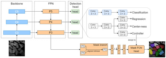
Figure 2.
Architecture of the proposed LosNet. In the feature pyramid networks (FPN), 1 × 1 convolutions are retained for feature channel dimension alignment extracted from the backbone. The detection head consists of four branches. The centerness branch is used to suppress the low-quality detected bounding boxes. The controller branch is used to generate the parameters of the mask full convolution network (FCN) head. In the mask branch, the feature maps P4 and P5 are added to P3 after the linear calculation. Then, these feature maps are input into the mask FCN head to obtain the final result.
3.2. Lightweight FPN
We propose the lightweight FPN to improve the inference speed and reduce the model size. It can be seen from Figure 3a that the feature maps of different scales complete channel alignment by a 1 × 1 convolution. After up-sampling, the feature maps with high semantic information are added to the corresponding feature maps. These feature maps are processed by a 3 × 3 convolution to obtain the P3, P4, and P5 layers. Then, two downsamples are taken from P5 to P6 and P7, respectively. It is well known that features of different scales have a superior influence on detecting objects of different sizes. However, the ores have been processed by an ore crusher. This demonstrates that the size of these ores is manageable. We no longer require small-scale feature maps in this scenario. Therefore, we choose to remove layers P6 and P7 from FPN.
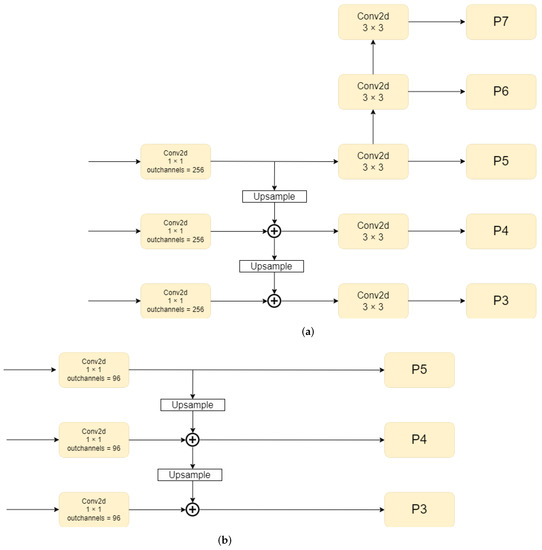
Figure 3.
Architecture of (a) original FPN and (b) our proposed lightweight FPN. In the original FPN network, the output has five layers: P3 to P7. In our proposed lightweight FPN, C3, C4, and C5 are processed to obtain P3, P4, and P5, with a 1 × 1 convolution and an up-sampling block.
For ore images, rich semantic information not only has little effect, but also increases the amount of computation. Reducing the number of channels and convolutions can achieve our needs for reducing extra semantic information. As a result, we propose a lightweight FPN, as shown in Figure 3b. First of all, we delete the 3 × 3 convolutions in FPN, which makes a significant contribution to our lightweight model. Then, we adjust the number of channels in the FPN. Since the number of channels needs to be kept at multiples of 8 or 16, the parallel acceleration of most inference frameworks can be enjoyed. The number of channels of 96 is a compromise between accuracy and model size. The number of parameters P can be calculated as P = . The parameter P of our method is 82,944, which is only 1/37 of the traditional FPN. We compare the feature maps of P3 of our proposed lightweight FPN and the original FPN to better highlight the performance of our suggested lightweight FPN. In Figure 4, the original FPN obtains more semantic information, resulting in more complex feature maps and more incorrect features. The feature maps produced by our proposed lightweight FPN are more concise, with no major loss of contour information.
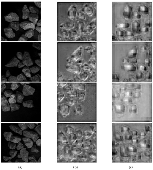
Figure 4.
(a) Input images; (b) rhe feature maps from the original FPN; (c) the feature maps from the lightweight FPN.
3.3. Optimized Detection Head
In the detection head, we use the centerness branch in parallel with the regression branch and controller branch to predict the centerness of a location, which can reduce the low-quality bounding boxes. The centerness depicts normalized distance from the location to the center of the object corresponding to that location. The centerness target is defined as,
where () and () represent the coordinates of the upper-left corner and the lower-right corner of the ground truth box, respectively, and (x, y) is the coordinate of each pixel.
In Equation (1), we employ sqrt to slow down the decay of the centerness. The centerness is trained with binary cross entropy (BCE) loss since it is between 0 and 1, which is added to the total loss function [32]. The final score is used to rank the detection targets in non-maximum suppression (NMS), which is defined as,
where the is the predicted centerness and the is the corresponding classification score. Centerness reduces the weight of the bounding box score away from the center of the object, which can increase the probability that these low-quality bounding boxes are filtered out by the final NMS process. The accuracy of LosNet can remain competitive with the help of centerness. To further decrease the computational cost, we simplify the network structure of the detection head. Since the input and output channels of the FPN are set to 96, the number of input channels is naturally consistent with the detection head.
In general, the most straightforward and effective technique to decrease model and computation is to reduce the number of convolutions. We can see from Figure 5a that the original detection head has a total of eight convolution layers, which is not acceptable for our lightweight model. We consider decreasing the four convolution groups in the detection head to two, as shown in Figure 5b. As a result, the detection head requires half the calculation that it does previously. Furthermore, we discovered that the original detection head uses group normalization as its method of normalization.
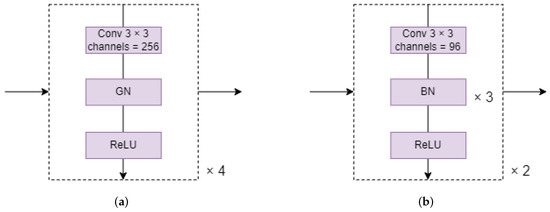
Figure 5.
(a) Original detection head and (b) our optimized detection head. The convolution layers in the original detector head and the optimized detector head are 4 and 2, respectively, and the number of input channels are 256 and 96, respectively. The original detection head consists of a 3 × 3 convolution layer, a GN layer, and ReLU, while our optimized detection head consists of a 3 × 3 convolution layer, three BN layers, and ReLU.
When comparing group normalization (GN) [33] to batch normalization (BN) [34], there is one disadvantage: BN can immediately integrate its normalized parameters into convolution during reasoning, allowing it to skip this part of the calculation, whereas GN cannot. We replaced GN with BN to reduce the time required for the normalization operation. In Figure 6, we compare the feature maps of the bounding box branches of our proposed optimized detection head and the original detection head to demonstrate the performance of our optimized detection head. The feature maps in Figure 6c are more accurate than those in Figure 6b.
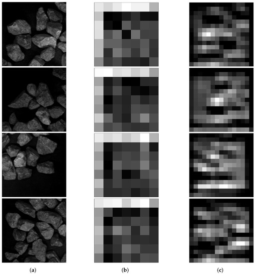
Figure 6.
(a) Input images. (b) The feature maps output from the original detection head. (c) The feature maps output from our optimized detection head.
3.4. Loss Function
Formally, the total loss function can be expressed as,
where and denote the loss for object detection and the loss for instance masks, respectively. To balance the two losses, is 1 in this work [26]. defined as,
where is focal loss [35] and is the generalized intersection over union (GIoU) loss [36]. is the number of locations where on the feature maps . is the indicator function, which is 1 if and 0 otherwise. and represent the classification scores and the regression prediction, respectively, for each location on the feature maps . defined as,
where is the classification label of location (x, y). is the class of the instance associated with the location; it is 0 if the location is not associated with any instance. is the parameter of the generated filter at location (x, y). is the combination of and a map of coordinates . is the relative coordinates from all the locations on to (x, y) (i.e., the location of generated filters). MaskHead denotes the mask head, which consists of a stack of convolutions with dynamic parameters . is the mask of the instance associated with location (x,y). is the dice loss as in [37], which is used to overcome the foreground–background sample imbalance. In Equation (5), we do not use focal loss because it requires special initialization. If the parameters are generated dynamically, it cannot be implemented. The predicted mask and the ground-truth mask are required to be the same size to compute the loss between them. The upsampling rate of the prediction is 4, so the resolution of the final prediction is half that of the ground truth mask . Accordingly, to make the sizes equal, we downsample by 2. These operations are omitted in Equation (5) for clarification.
4. Experiments
In this section, we first introduce the ore datasets and evaluation metrics. Then, we perform ablation studies to dissect our various design choices. Finally, we compare our LosNet with the state-of-the-art methods for instance segmentation.
4.1. Experiments Setup
4.1.1. Implementation Details
Unless otherwise specified, we use the following implementation details. All models were trained on a single GTX2080Ti GPU for 18K iterations with an initial learning rate of 0.01 and a mini-batch of 20 images. During training, the input photographs were altered to have shorter sides in the range [300, 480] and longer sides less than or equal to 640 pixels. During testing, we did not use any data augmentation and the scale of shorter and longer sides used was 640 and 800, respectively. We utilized a batch size of 4 in the experiments in Section 4.2 and Section 4.3. The inference time and inference memory usage were measured on a single GTX2080Ti GPU.
4.1.2. Datasets
We supplemented ore datasets in the following ways. First, we gathered ore pictures at various scales. Then, on various scales, we altered the positioning of ores, such as sparse, thick, etc. Furthermore, we partitioned large photos into small images that can be used in network training. To boost the number of datasets even further, we split images with a sliding window in Figure 7. We used 4060 images for training and 1060 images for validating. Stacking, sticky, and occulting between ores are all serious issues that complicated our task. The ores in the second row of images are denser and brighter than those in the first row.
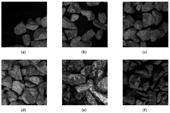
Figure 7.
(a–d) depict ore images with varying densities under the same light. (e) is a different type of ore image with a smaller ore volume. (f) depicts the ore image in low light.
4.1.3. Evaluation Metrics
There are 11 indexes [12,13] that were used to verify the effectiveness of the proposed LosNet, i.e., , , , , , , training speed, training memory usage, inference memory usage, inference speed, and model size. Accuracy was measured using the top six indexes. The computational expenses of the model are reflected in the inferred speed. When computing power is limited, we prefer models with minimal computational costs and fast detection speeds. The memory usage of a model during training demonstrates the reliance on the hardware system. The last three indexes are critical in determining if a model may be deployed on modest equipment.
4.2. Backbone
To test the effectiveness of our LosNet, we first analyzed the network’s overall structure. For experimentation, we replaced the baseline network with other backbones, using our ore dataset as an example. The goal of our framework is to achieve lightweight and real-time performance while maintaining competitive accuracy. As shown in Table 1, ResNet50 has the highest accuracy, but its model size and inference time are 259 MB and 56.7 ms, respectively. Despite having the smallest model size, its inference time reaches 49.9 ms. MobileNetV3-Small has an accuracy of 61.49 in and 47.85 in , while its model size and inference time are only 89 MB and 35.9 ms, respectively. Furthermore, the inference memory usage of MobileNetV3-Small is the smallest in all backbones. Therefore, we chose MobileNetV3-Small as the backbone of our LosNet.

Table 1.
Comparison of different backbones.
4.3. Ablation Study
The following ablation experiments were performed on the MobileNetV3-small [30]. In addition, we reserve two significant figures in the accuracy results to clearly indicate the results of the ablation experiment.
4.3.1. FPN Structure Design
To compress the model size, we reduced the number of input channels in the FPN and deleted the internal 3 × 3 convolution. In Table 2, we performed ablation experiments on the number of FPN input channels. Similarly, we also conducted the same experiment on the FPN after deleting the 3 × 3 convolution. This allows us to demonstrate our impact on FPN improvement in a more intuitive manner. The first two requirements for this task are small models and high speeds; thus, we reduce the number of channels from 128 to 64 at 32 channel intervals.
Table 2.
Comparisons of different channels. Channels represents the number of input channels in FPN and convs. represents 3 × 3 convolutions in the FPN.
In Table 2, with 3 × 3 convolution preserved, 128 channels achieves 48.05% in . When the number of channels decreases from 128 to 96, the performance is improved by 0.8 ms in inference time, and the model size is reduced by 8 MB. When the number of channels decreases from 96 to 64, the performance is improved by 1 ms, and model size is reduced by 6 MB. However, the loss of the latter is 2.75× higher than that of the former (0.22% vs. 0.08% in ). The reason for this is that too much useful information is lost in 64 channels and too much redundant information is obtained in 256 channels. Therefore, deleting the 3 × 3 convolution with fewer channels has little effect on accuracy and speed. Therefore, when the number of channels is 96, we achieve the benefit of model downsizing by 1 MB without any loss.
Due to the characteristics of mineral images, most of the small-scale information in the FPN is redundant. From Table 3, we can see that all metrics are improved after deleting P6 and P7. It is reasonable and feasible to delete the P6 and P7 layers. Without the P6 and P7 layers, the amount of calculation of the model is reduced, so the model size is reduced from 89 MB to 80 MB. Meanwhile, discarding redundant and incorrect semantics leads to improved accuracy ( increases from 61.49% to 61.90%, and increases from 47.85% to 47.95%). Most importantly, the inference time reaches 31.0 ms after deleting P6 and P7, which makes a large contribution to the real-time implementation of our method.
Table 3.
Ablation study of P6 and P7 layer in the FPN.
4.3.2. Design of Detection Head
As discussed above, there is only one category in the ore images. In this case, too many convolutions can easily lead to an excessive interpretation of image information by the network. Therefore, it is necessary to discuss the number of convolution layers in the bounding box regression branch and classification branch in the detection head.
As shown in Table 4, when the number of convolution layers is 2, is only reduced by 0.63%. At the same time, the inference time is reduced by 4.3 ms and the model size is reduced by 18 MB. When the number of convolutional layers is reduced from 4 to 1, the improvement amplitude of inference time and model size begins to decrease. However, the decreases significantly by 3.07%. It is worth noting that the is improved when the number of convolutions is reduced. Similarly, when the number of convolutional layers is 2, the increases the most. Therefore, the most appropriate number of convolution layers in the bounding box regression branch and classification is 2. We obtain the maximum return with minimum loss of . The is increased from 61.49% to 66.20%, the inference time is reduced from 35.9 ms to 31.6 ms, and the model size is reduced from 89 MB to 71 MB.
Table 4.
Design of convolution number in bounding box regression and classification branches.
In Table 5, we compare the two mainstream normalization methods (GN and BN). Inference time reduces from 35.9 ms to 33.4 ms, but the and decrease from 61.49% and 47.85% to 60.65% and 47.63%, respectively. It is difficult to avoid the loss of accuracy in exchange for the improvement of speed, and a small loss of accuracy is acceptable. It is reasonable to replace GN with BN to increase inference speed.
Table 5.
Comparison of group normalization (GN) and batch normalization (BN). Norm. represents the normalization method.
4.3.3. Lightweight FPN vs. Original FPN
We compare the two FPNs on our LosNet framework to demonstrate the difference between the original FPN and our lightweight FPN. Table 6 shows that the accuracy of LosNet is increased by 0.41 in with the help of the lightweight FPN and the inference time and model size are lowered by 4.5 ms and 45 MB, respectively. Simultaneously, the accuracy is only reduced by 0.1 in . This demonstrates the significance and effectiveness of our lightweight FPN.
Table 6.
Ablation study of lightweight FPN and original FPN.
4.4. Comparison with State-of-the-Art Methods
To further illustrate the superiority of our LosNet, we compare our framework with the state-of-the-art methods, e.g., Mask R-CNN [12], mask scoring R-CNN (MS R-CNN) [17], CARAFE [21], cascade mask R-CNN (CM R-CNN) [47], HTC [18], GRoIE [23], SCNet [22], YOLACT [13], BlendMask [24], CondInst [26], SOLOv2 [27], and BoxInst [29]. As shown in Table 8, the inference time of all methods was calculated on a NVIDIA 2080ti and the parameters in each method were tuned to achieve the best performance on our datasets. In Table 7 and Table 8, “RX-101”, “R2-101”, “S-50”, and “M-V3s” refer to ResNeXt-101 [48], Res2Net-101 [49], ResNeSt [50], and MobileNetV3-small [30], respectively.
Table 7.
Comparison of accuracy with the state-of-the-art methods on ore image datasets.
Table 8.
Comparison of the speed, memory, and model size with the state-of-the-art methods on ore image datasets.
In Table 7, LosNet performs well in and . When LosNet takes MobileNetV3-small as the backbone, the is higher than all other algorithms. Although LosNet with MobileNetV3-small is 2.87% lower than Cascade Mask R-CNN in , the model size of Cascade Mask R-CNN is 22× larger than LosNet. The inference time of LosNet is only 1/3 of that of Cascade R-CNN. The inference time of LosNet is only about 25 ms (40 FPS, while even YOLACT needs 33 ms (30 FPS) of inference time with the help of ResNet-50. Furthermore, the model size of LosNet is only 26 MB, which shows that our method has the ability to be deployed on edge devices. The model size of other methods is at least 10× that of ours. Furthermore, we can also see that our LosNet performs best in training time and memory usage in Table 8.
LosNet performs best in model size and inference time with the same backbone, ResNet-50. With such excellent performance, our method is only 0.41% lower than Cascade Mask R-CNN in . LosNet performs better than YOLACT in all indexes (e.g., 56.6% vs. 50.5% in , 49.2% vs. 11.5% in , 32 ms vs. 33 ms in inference time, 193 MB vs. 256 MB in model size). The accuracy of our method is higher than CondInst and the inference time and model size are also much smaller than CondInst. As shown in Figure 8, we analyzed the ore images in different situations. LosNet can still obtain high-quality instance segmentation results even when there is stacking and stickiness.
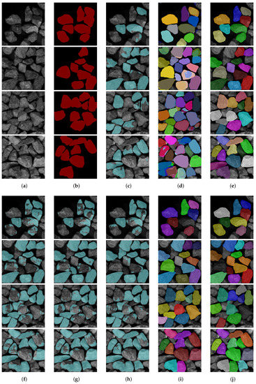
Figure 8.
The visual results of ore images processed by different methods. (a) Original picture; (b) ground truth; (c) YOLACT; (d) SOLOv2; (e) CondInst; (f) Mask R-CNN; (g) MS R-CNN; (h) CARAFE; (i) LosNet(R-50); (j) LosNet(M-V3).
5. Conclusions
We developed a real-time system for ore image analysis. More specially, we put forward the LosNet framework for instance segmentation of ore images to discern full and independent ores. This framework includes a lightweight backbone and a lightweight FPN to simultaneously reduce unnecessary semantic information and computation. Moreover, we suggest an improved detection head to maintain the accuracy of our framework. Experiments on ore image datasets demonstrate that our proposed LosNet can achieve real-time speed of 40 FPS with a small model size of 26 MB. Meanwhile, our LosNet retains competitive accuracy performance, i.e., 67.68% in and 46.73% in , in comparison with the state-of-the-art methods.
In the future, we plan to apply our model to edge computing devices to address the needs of practical engineering. We will keep improving accuracy and speed while reducing model size.
Author Contributions
Conceptualization, G.S.; data curation, D.H., L.C., J.J. and C.X.; methodology, D.H., L.C. and Y.Z.; project administration, G.S. and Y.Z.; writing—original draft, D.H., L.C. and Y.Z.; writing—review and editing, G.S., D.H. and Y.Z.; funding acquisition, G.S. All authors have read and agreed to the published version of the manuscript.
Funding
This work was supported in part by the National Natural Science Foundation of China (Grant 51775177) and the PhD early development program of Hubei University of Technology (Grant XJ2021003801).
Data Availability Statement
Not applicable.
Conflicts of Interest
The authors declare no conflict of interest.
References
- Ma, X.; Zhang, P.; Man, X.; Ou, L. A New Belt Ore Image Segmentation Method Based on the Convolutional Neural Network and the Image-Processing Technology. Minerals 2020, 10, 1115. [Google Scholar] [CrossRef]
- Wang, R.; Zhang, W.; Shao, L. Research of ore particle size detection based on image processing. In Proceedings of the 2017 Chinese Intelligent Systems Conference (CISC 2017), MudanJiang, China, 14–15 October 2017; Lecture Notes in Electrical Engineering Series; Springer: Singapore, 2018; Volume 460, pp. 505–514. [Google Scholar]
- Amankwah, A.; Aldrich, C. Automatic ore image segmentation using mean shift and watershed transform. In Proceedings of the 21st International Conference Radioelektronika 2011, Brno, Czech Republic, 19–20 April 2011; pp. 245–248. [Google Scholar]
- Dong, K.; Jiang, D. Automated estimation of ore size distributions based on machine vision. In Unifying Electrical Engineering and Electronics Engineering; Lecture Notes in Electrical Engineering Series; Springer: New York, NY, USA, 2014; Volume 238, pp. 1125–1131. [Google Scholar]
- Chalfoun, J.; Majurski, M.; Dima, A.; Stuelten, C.; Peskin, A.; Brady, M. FogBank: A single cell segmentation across multiple cell lines and image modalities. BMC Bioinform. 2014, 15, 431. [Google Scholar] [CrossRef] [PubMed] [Green Version]
- Lu, Z.M.; Zhu, F.C.; Gao, X.Y.; Chen, B.C.; Gao, Z.G. In-situ particle segmentation approach based on average background modeling and graph-cut for the monitoring of l-glutamic acid crystallization. Chemom. Intell. Lab. Syst. 2018, 178, 11–23. [Google Scholar] [CrossRef]
- Zhang, G.Y.; Liu, G.Z.; Zhu, H.; Qiu, B. Ore image thresholding using bi-neighbourhood Otsu’s approach. Electron. Lett. 2010, 46, 1666–1668. [Google Scholar] [CrossRef]
- Malladi, S.R.S.P.; Ram, S.; Rodriguez, J.J. Superpixels using morphology for rock image segmentation. In Proceedings of the IEEE Southwest Symposium on Image Analysis and Interpretation, San Diego, CA, USA, 6–8 April 2014; pp. 145–148. [Google Scholar]
- Mukherjee, D.P.; Potapovich, Y.; Levner, I.; Zhang, H. Ore image segmentation by learning image and shape features. Pattern Recognit. Lett. 2009, 30, 615–622. [Google Scholar] [CrossRef]
- Wei, W.; Li, Q.; Xiao, C.; Zhang, D.; Miao, L.; Wang, L. An Improved Boundary-Aware U-Net for Ore Image Semantic Segmentation. Sensors 2021, 21, 2615. [Google Scholar]
- Menshchikov, A.; Shadrin, D.; Prutyanov, V.; Lopatkin, D.; Sosnin, S.; Tsykunov, E.; Iakovlev, E.; Somov, A. Real-Time Detection of Hogweed: UAV Platform Empowered by Deep Learning. IEEE Trans. Comput. 2021, 70, 1175–1188. [Google Scholar] [CrossRef]
- He, K.; Gkioxari, G.; Dollár, P.; Girshick, R. Mask R-CNN. In Proceedings of the IEEE International Conference on Computer Vision (ICCV), Venice, Italy, 22–29 October 2017; pp. 2980–2988. [Google Scholar]
- Bolya, D.; Zhou, C.; Xiao, F.; Lee, Y.J. YOLACT: Real-Time Instance Segmentation. In Proceedings of the IEEE/CVF International Conference on Computer Vision (ICCV), Seoul, Korea, 27 October–2 November 2019; pp. 9156–9165. [Google Scholar]
- Yang, G.Q.; Wang, H.G.; Xu, W.; Li, P.C.; Wang, Z.M. Ore particle image region segmentation based on multilevel strategy. Chin. J. Anal. Lab. 2014, 35, 202–204. [Google Scholar]
- Zhang, B.; Mukherjee, R.; Abbas, A.; Romagnoli, J. Multi-resolution fuzzy clustering approach for image-based particle characterization. IFAC Proc. Vol. 2010, 43, 153–158. [Google Scholar] [CrossRef]
- Ren, S.; He, K.; Girshick, R.; Sun, J. Faster R-CNN: Towards Real-Time Object Detection with Region Proposal Networks. IEEE Trans. Pattern Anal. Mach. Intell. 2017, 39, 1137–1149. [Google Scholar] [CrossRef] [PubMed] [Green Version]
- Huang, Z.; Huang, L.; Gong, Y.; Huang, C.; Wang, X. Mask scoring R-CNN. In Proceedings of the IEEE/CVF Conference on Computer Vision and Pattern Recognition (CVPR), Long Beach, CA, USA, 15–20 June 2019; pp. 6402–6411. [Google Scholar]
- Chen, K.; Pang, J.; Wang, J.; Xiong, Y.; Li, X.; Sun, S.; Feng, W.; Liu, Z.; Shi, J.; Ouyang, W.; et al. Hybrid Task Cascade for Instance Segmentation. In Proceedings of the IEEE/CVF Conference on Computer Vision and Pattern Recognition (CVPR), Long Beach, CA, USA, 15–20 June 2019; pp. 4969–4978. [Google Scholar]
- Kuo, W.; Angelova, A.; Malik, J.; Lin, T.Y. ShapeMask: Learning to Segment Novel Objects by Refining Shape Priors. In Proceedings of the IEEE/CVF International Conference on Computer Vision (ICCV), Seoul, Korea, 27 October–2 November 2019; pp. 9206–9215. [Google Scholar]
- Liang, J.; Homayounfar, N.; Ma, W.C.; Xiong, Y.; Hu, R.; Urtasun, R. PolyTransform: Deep Polygon Transformer for Instance Segmentation. In Proceedings of the IEEE/CVF International Conference on Computer Vision and Pattern Recognition (CVPR), Seattle, WA, USA, 13–19 June 2020; pp. 9128–9137. [Google Scholar]
- Wang, J.; Chen, K.; Xu, R.; Liu, Z.; Loy, C.C.; Lin, D. CARAFE: Content-Aware ReAssembly of FEatures. In Proceedings of the IEEE/CVF International Conference on Computer Vision (ICCV), Seoul, Korea, 27 October–2 November 2019; pp. 3007–3016. [Google Scholar]
- Vu, T.; Kang, H.; Yoo, C.D. SCNet: Training Inference Sample Consistency for Instance Segmentation. arXiv 2020, arXiv:2012.10150. [Google Scholar]
- Rossi, L.; Karimi, A.; Prati, A. A Novel Region of Interest Extraction Layer for Instance Segmentation. In Proceedings of the 25th International Conference on Pattern Recognition (ICPR), Milan, Italy, 10–15 January 2021; pp. 2203–2209. [Google Scholar]
- Chen, H.; Sun, K.; Tian, Z.; Shen, C.; Huang, Y.; Yan, Y. BlendMask: Top-Down Meets Bottom-Up for Instance Segmentation. In Proceedings of the IEEE/CVF International Conference on Computer Vision and Pattern Recognition (CVPR), Seattle, WA, USA, 13–19 June 2020; pp. 8570–8578. [Google Scholar]
- Wang, Y.; Xu, Z.; Shen, H.; Cheng, B.; Yang, L. CenterMask: Single Shot Instance Segmentation With Point Representation. In Proceedings of the IEEE/CVF International Conference on Computer Vision and Pattern Recognition (CVPR), Seattle, WA, USA, 13–19 June 2020; pp. 9310–9318. [Google Scholar]
- Tian, Z.; Shen, C.; Chen, H. Conditional Convolutions for Instance Segmentation. In Proceedings of the 16th European Conference on Computer Vision (ECCV 2020), Glasgow, UK, 23–28 August 2020; pp. 282–298. [Google Scholar]
- Wang, X.; Zhang, R.; Kong, T.; Li, L.; Shen, C. SOLOv2: Dynamic and fast instance segmentation. In Proceedings of the 34th Conference on Neural Information Processing Systems (NeurIPS 2020), Vancouver, BC, Canada, 6–12 December 2020. [Google Scholar]
- Wang, X.; Zhang, R.; Shen, C.; Kong, T.; Li, L. SOLO: A Simple Framework for Instance Segmentation. IEEE Trans. Pattern Anal. Mach. Intell. 2021, in press. [Google Scholar] [CrossRef] [PubMed]
- Tian, Z.; Shen, C.; Wang, X.; Chen, H. BoxInst: High-Performance Instance Segmentation with Box Annotations. In Proceedings of the IEEE/CVF International Conference on Computer Vision and Pattern Recognition (CVPR), Nashville, TN, USA, 20–25 June 2021; pp. 5439–5448. [Google Scholar]
- Howard, A.; Sandler, M.; Chen, B.; Wang, W.; Chen, L.C.; Tan, M.; Chu, G.; Vasudevan, V.; Zhu, Y.; Pang, R.; et al. Searching for MobileNetV3. In Proceedings of the IEEE/CVF International Conference on Computer Vision (ICCV), Seoul, Korea, 27 October–2 November 2019; pp. 1314–1324. [Google Scholar]
- Lin, T.Y.; Dollár, P.; Girshick, R.; He, K.; Hariharan, B.; Belongie, S. Feature Pyramid Networks for Object Detection. In Proceedings of the IEEE International Conference on Computer Vision and Pattern Recognition (CVPR), Honolulu, HI, USA, 21–26 July 2017; pp. 936–944. [Google Scholar]
- Tian, Z.; Shen, C.; Chen, H.; He, T. FCOS: Fully Convolutional One-Stage Object Detection. In Proceedings of the IEEE/CVF International Conference on Computer Vision (ICCV), Seoul, Korea, 27 October–2 November 2019; pp. 9626–9635. [Google Scholar]
- Wu, Y.; He, K. Group Normalization. Int. J. Comput. Vis. 2020, 128, 742–755. [Google Scholar] [CrossRef]
- Ioffe, S.; Szegedy, C. Batch normalization: Accelerating deep network training by reducing internal covariate shift. In Proceedings of the 32nd International Conference on Machine Learning (ICML 2015), Lille, France, 6–11 July 2015; Volume 1, pp. 448–456. [Google Scholar]
- Lin, T.Y.; Goyal, P.; Girshick, R.; He, K.; Dollár, P. Focal Loss for Dense Object Detection. IEEE Trans. Pattern Anal. Mach. Intell. 2020, 42, 318–327. [Google Scholar] [CrossRef] [PubMed] [Green Version]
- Rezatofighi, H.; Tsoi, N.; Gwak, J.; Sadeghian, A.; Reid, I.; Savarese, S. Generalized Intersection Over Union: A Metric and a Loss for Bounding Box Regression. In Proceedings of the IEEE/CVF International Conference on Computer Vision and Pattern Recognition (CVPR), Long Beach, CA, USA, 15–20 June 2019; pp. 658–666. [Google Scholar]
- Milletari, F.; Navab, N.; Ahmadi, S.A. V-Net: Fully Convolutional Neural Networks for Volumetric Medical Image Segmentation. In Proceedings of the Fourth International Conference on 3D Vision, Stanford, CA, USA, 25–28 October 2016; pp. 565–571. [Google Scholar]
- Yu, F.; Wang, D.; Shelhamer, E.; Darrell, T. Deep Layer Aggregation. In Proceedings of the IEEE/CVF Conference on Computer Vision and Pattern Recognition, Salt Lake City, UT, USA, 18–23 June 2018; pp. 2403–2412. [Google Scholar]
- Tan, M.; Le, Q. EfficientNet: Rethinking Model Scaling for Convolutional Neural Networks. In Proceedings of the 36th International Conference on Machine Learning, Long Beach, CA, USA, 9–15 June 2019; pp. 6105–6114. [Google Scholar]
- Tan, M.; Chen, B.; Pang, R.; Vasudevan, V.; Sandler, M.; Howard, A.; Le, Q.V. MnasNet: Platform-Aware Neural Architecture Search for Mobile. In Proceedings of the IEEE/CVF International Conference on Computer Vision and Pattern Recognition (CVPR), Long Beach, CA, USA, 15–20 June 2019; pp. 2815–2823. [Google Scholar]
- Sandler, M.; Howard, A.; Zhu, M.; Zhmoginov, A.; Chen, L.C. MobileNetV2: Inverted Residuals and Linear Bottlenecks. In Proceedings of the IEEE/CVF Conference on Computer Vision and Pattern Recognition, Salt Lake City, UT, USA, 18–23 June 2018; pp. 4510–4520. [Google Scholar]
- He, K.; Zhang, X.; Ren, S.; Sun, J. Deep Residual Learning for Image Recognition. In Proceedings of the IEEE Conference on Computer Vision and Pattern Recognition (CVPR), Las Vegas, NV, USA, 27–30 June 2016; pp. 770–778. [Google Scholar]
- Lee, Y.; Hwang, J.; Lee, S.; Bae, Y.; Park, J. An Energy and GPU-Computation Efficient Backbone Network for Real-Time Object Detection. In Proceedings of the IEEE/CVF Conference on Computer Vision and Pattern Recognition Workshops (CVPRW), Long Beach, CA, USA, 16–17 June 2019; pp. 752–760. [Google Scholar]
- Wang, R.J.; Li, X.; Ling, C.X. Pelee: A Real-Time Object Detection System on Mobile Devices. In Proceedings of the 32nd International Conference on Neural Information Processing Systems, Montreal, QC, Canada, 3–8 December 2018; pp. 1967–1976. [Google Scholar]
- Radosavovic, I.; Kosaraju, R.P.; Girshick, R.; He, K.; Dollar, P. Designing network design spaces. In Proceedings of the IEEE/CVF International Conference on Computer Vision and Pattern Recognition (CVPR), Seattle, WA, USA, 13–19 June 2020; pp. 10425–10433. [Google Scholar]
- Ma, N.; Zhang, X.; Zheng, H.T.; Sun, J. ShuffleNet V2: Practical Guidelines for Efficient CNN Architecture Design. In Computer Vision—ECCV 2018, Proceedings of the 15th European Conference, Munich, Germany, 8–14 September 2018; Lecture Notes in Computer Science Series; Springer: Cham, Switzerland, 2018; pp. 122–138. [Google Scholar]
- Cai, Z.; Vasconcelos, N. Cascade R-CNN: High Quality Object Detection and Instance Segmentation. IEEE Trans. Pattern Anal. Mach. Intell. 2021, 43, 1483–1498. [Google Scholar] [CrossRef] [PubMed] [Green Version]
- Xie, S.; Girshick, R.; Dollár, P.; Tu, Z.; He, K. Aggregated Residual Transformations for Deep Neural Networks. In Proceedings of the IEEE International Conference on Computer Vision and Pattern Recognition (CVPR), Honolulu, HI, USA, 21–26 July 2017; pp. 5987–5995. [Google Scholar]
- Gao, S.H.; Cheng, M.M.; Zhao, K.; Zhang, X.Y.; Yang, M.H.; Torr, P. Res2Net: A New Multi-Scale Backbone Architecture. IEEE Trans. Pattern Anal. Mach. Intell. 2021, 43, 652–662. [Google Scholar] [CrossRef] [PubMed] [Green Version]
- Zhang, H.; Wu, C.; Zhang, Z.; Zhu, Y.; Zhang, Z.; Lin, H.; Sun, Y.; He, T.; Mueller, J.; Manmatha, R.; et al. ResNeSt: Split-Attention Networks. arXiv 2020, arXiv:2004.08955. [Google Scholar]
Publisher’s Note: MDPI stays neutral with regard to jurisdictional claims in published maps and institutional affiliations. |
© 2022 by the authors. Licensee MDPI, Basel, Switzerland. This article is an open access article distributed under the terms and conditions of the Creative Commons Attribution (CC BY) license (https://creativecommons.org/licenses/by/4.0/).