Article

Simulation Algorithm for Water Elutriators: Model Calibration with Plant Data and Operational Simulations

1
Department of Mining, Metallurgy & Materials Engineering, University Laval, Québec, QC G1V 0A6, Canada
2
Department of Chemical Engineering, University Laval, Québec, QC G1V 0A6, Canada
*
Author to whom correspondence should be addressed.
Minerals 2022, 12(3), 316; https://doi.org/10.3390/min12030316
Submission received: 31 January 2022 / Revised: 22 February 2022 / Accepted: 25 February 2022 / Published: 1 March 2022

Abstract

:
A dynamic simulation algorithm based on 1-D transient convection/diffusion transport per particle size class is proposed to simulate a hydraulic classifier operated to selectively remove quartz from an iron oxide concentrate produced by processing the ore from an iron ore mine in northeastern Canada. The calibrated model is used to simulate the operation of dense bed hydraulic classifiers of different sizes and/or under different operating conditions. The simulator predicts the behavior and characteristics of the pulp at different depths within the classifier as a function of time. The simulator is validated by confronting the simulation results to experimental data obtained from sampling industrial and laboratory classifiers. The simulator is then used to assess the role of the fluidization or teeter water and of bed density on the quality of the produced separation of quartz from the valuable iron oxide of the processed ore. The knowledge acquired in the noise-free environment of simulation provides clues on the way to manipulate the hydraulic classifier operating variables in a process control strategy for an industrial scale unit.

1. Introduction

Mineral concentration processes refer to the operations used to separate the valuable minerals from the non-valuable minerals (gangue) in mined ores or rocks. Mineral concentration equipment either use the physical (specific gravity, magnetic susceptibility, electrical conductivity, etc.) or chemical (surface composition) properties of the minerals to achieve their separation [1]. Reliance on the differences in the specific gravities between valuable and non-valuable minerals is certainly the oldest and most traditional way to carry out such separations. Gravity separation devices are inexpensive to operate and do not require the addition of chemical reagents to carry out the separation of valuable minerals from the gangue and are thus often considered as environmentally friendly (Burt, 1999 [2]). Das and Sakar (2018, [3]) present a review of gravimetric concentration processes. The present study focuses on a type of gravity separation equipment named hydraulic classifier (Hc) or water elutriator.
The different types of hydraulic classifiers are presented in the work of Tripathy et al. [4] and the one studied here is the floatex density separator. Hc units have been the subject of several studies and publications (Bazin et al. 2011–2012 [5,6], Das et al. 2007–2010 [7,8,9,10]; Sar et al. 2017 [11]; Sadeghi and Bazin 2020 [12], among others). Generally, the prevailing separation mechanisms in an Hc are hindered settling, elutriation and fluidization [4,13]. These separators consist of continuously-fed units that can process large amounts of solids and generate dense fluidized particle beds that can greatly improve the separation acuity (Galvin et al., 1999 [14]). Hc combines low capital installation and operating costs (Luttrell et al., [13]) and should therefore always be considered as an economically viable option for the separation of minerals.
The main objective of the study is to develop a phenomenological model that explicitly accounts for the common operating variables (flow rate of the teeter water, bed density, and so forth) of the classifier and the geometric characteristics of the apparatus. The proposed mathematical model can help the operators to improve the operation of existing processes by simulating the performances of different control strategies or by predicting the performances of separation equipment prior to its commissioning into a circuit consisting of several gravity separators. The separation of particles in an Hc results from a combination of particle size and specific gravity effects given the properties of the liquid (density, viscosity), which is often an aqueous base. Indeed, a coarse and low-density non-valuable mineral particle may behave similarly to a small and dense heavy valuable mineral particle, making it difficult to anticipate the classifier’s separation quality without pilot-scale testing of the ore under scrutiny. However, multiplication of pilot-scale testing may rapidly lead to an increase in the costs of a pre-feasibility study. Hence, the development and use of virtual mathematically-based models for industrial equipment are certainly viewed as the ‘voie royale’ to help reduce the risk associated with the commissioning of a circuit incorporating that equipment or to assist plant operators in designing a control strategy for the existing operating equipment.
The objective of this paper is to propose an Hc mathematical model that can serve the two indicated purposes, namely, design and optimization. To establish the material balance of the Hcs, the algorithm considers that the volume flow of material is the resultant of the forces generated from dispersion and convection (hindered settling or elutriation). This relationship is used, among others, for the simulation of hydraulic classifiers [15,16,17] and for the simulation of fluidized beds [18,19,20,21,22,23]. The use of the dispersion term allows the modification of the velocity profile of the solid particles, which results from a non-uniform flow profile of the liquid, a mixing effect caused by the turbulence of the flow and the rebalancing of the density gradient as a function of height by the Archimedes’ principle, while the convection term allows to model the effect of gravity forces and the movement of the surrounding medium. The method of solving the equation of motion, which is a partial derivative equation, is inspired by the research works of Kim [15], Lee [23] and Honaker [16]. The combination of their solution methods results in a computational algorithm with high stability when there is a large variation of the solid concentration according to the depth.
More recently, Payenzo et al. (2011, [5]) analyzed the operation of an Hc for iron ores using the partition or efficiency curves of the minerals. However, their investigation was limited to simply observing the actual operation of the classifier. The authors concluded on the limited applicability of their model, as it was not possible to use their approach to simulate the response of the classifier to actions implemented on the two main operating variables of the classifier, namely, the density of the bed and the flow rate of the fluidization water. Most of the mathematical models proposed so far for the hydraulic classifiers do not explicitly account for all operating variables of the classifier (feed water and underflow), a weakness that the model proposed in this study attempts to overcome. Unlike many previous studies dealing with hydraulic classifiers that analyze the behavior of spheres in water, this study is concerned with the modeling of an industrial unit processing an actual ore. Despite the fact that gravity separation devices have been operating for eons, there is still no well-established mathematical representation for an industrial Hc. To improve the modeling of the behavior of industrial Hc, it was necessary to introduce new concepts, such as the convection generated by the underflow, supervision and control of simulation variables (concentration, underflow rate and pulp density) and the addition of methods for estimating the parameters of the model (bed porosity and axial dispersion coefficient). The developed mathematical model does not require physical assembly to be simulated and can help operators to improve designs using hydraulic classifiers, allowing the simulation of different control strategies and the design of equipment for particular applications. In addition, the simulation tool allows the prediction of the states of unmeasured and/or unmeasurable variables, such as local density, overflow composition and interface location, thus allowing it to be used as a virtual sensor.

2. Materials and Methods

2.1. Sampling the Industrial Hydraulic Classifier

Most of the data used for the development of the model for the Hc come from the sampling of the industrial Hc units. A sampling campaign on a hydraulic classifier usually lasts less than one hour. The hydraulic classifier was first allowed to operate under steady state during one hour before starting to collect samples from the feed, underflow and overflow streams. Each stream was cut three times during the one-hour sampling campaign and the cuts were combined to give the composite samples used for the analysis.
The samples were analyzed to obtain the slurry solids’ concentration, the elemental (Fe, SiO2, Al2O3, CaO, Na2O, MgO, etc.) composition and the particle size distribution of the solids. The material within each size fraction was assayed for the same elements as the head sample. The data were finally processed using a material balance program that calculates the solids split between the Hc underflow and overflow streams. The materiel balance algorithm was also built to calculate the mineral (hematite, magnetite, quartz, mica, garnet, ilmenite, etc.) concentrations from the elemental assays for the three sampled streams of the Hc [24,25]. The estimated mineral concentrations and the solid split were used to calculate the previously defined performance indices.
Samples were also collected during steady-state operation at various depths inside the Hc in order to evaluate the type of mixing along the vertical axis. These samples were analyzed to obtain the slurry solids’ concentration and the elemental composition. The results of this sampling, shown in Figure 1, clearly demonstrate [24] that the concentration of solids and the density of the pulp vary with depth and that the mixing within a Hc is clearly not that of a perfect mixer justifying the discretization approach used here for the model development.
The operating principle of the mine, concentrator and pellet plant is detailed in Appendix A.1. Appendix A.2 explains the operation of the Hcs in the pellet plant, while Appendix A.3 discusses the performance indices used to describe the separation efficiency.

Analytical Methods

The solid samples were assayed using a Pananalytical Epsilon 1 Energy Dispersive X-Ray Fluorescence (ED-XRF) (Malvern Panalytical, Westborough, MA, USA). XRF samples were fused with lithium Borax to prepare glasses for the chemical analysis. The mineral composition of the samples obtained from the tests conducted on the laboratory set-up was back calculated from the density of the sample, as measured using a Gas pycnometer (HumiPyc model 2 from Instruquest, Boca Raton, FL, USA). The size distribution of a sample was measured by using Tyler screens ranging from 1200 to 38 µm.

2.2. Laboratory Set-Up

In order to verify the versatility of the simulation algorithm in various situations (geometry, pulp characteristics, flow regime, etc.), experiments were also carried out using a laboratory unit [24]. Table 1 gives the characteristics and operating conditions for the laboratory set-up and presents an average value of the operating parameters of the Hcs of the pellet plant in Port-Cartier. The first experimental step in the laboratory set-up was to mix the solid and water in the feed tank. Once this step was completed, the hydraulic classifier was filled with water using the cone water and teeter water injectors. Afterwards, the feed, cone water and teeter water flow rates were set to the selected value for the experiment. Once the system was started, it was operated for 30 min to allow a steady state to be reached, before taking the first samples. The obtained samples were then weighed, dried and sieved. The last step consists in determining the density of the solid using a gas pycnometer (HumiPyc). This last step allows to estimate the proportion of heavy and light particles of the sample.

3. Mathematical Model

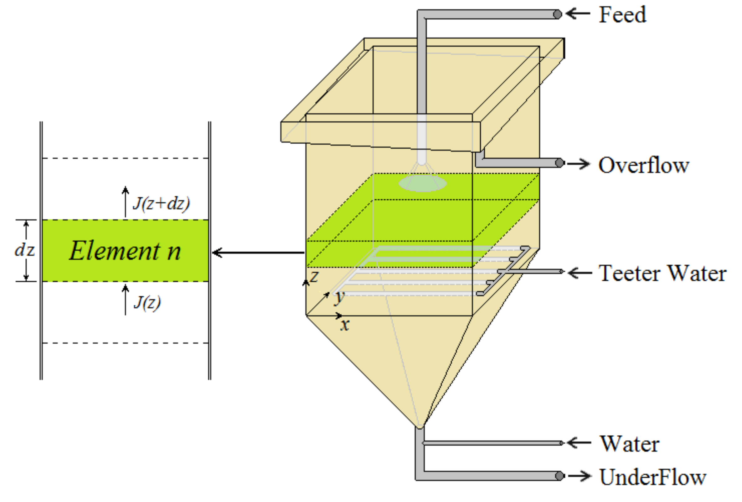
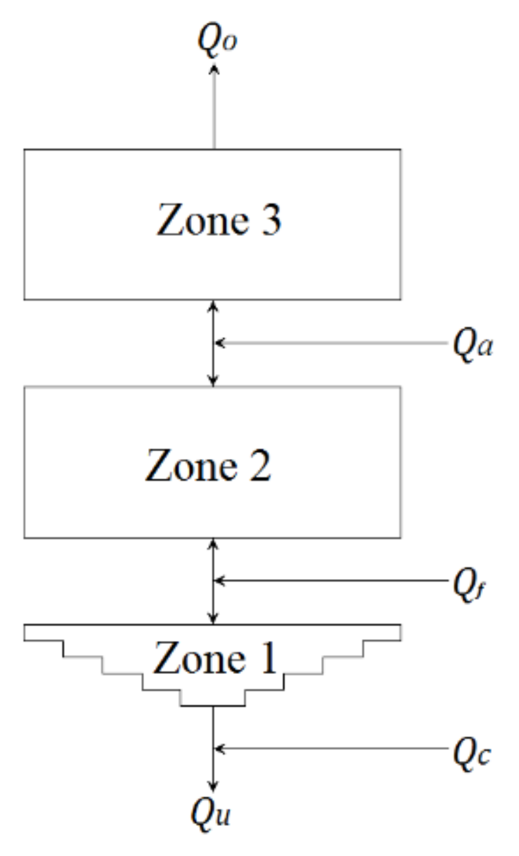
3.1. 1-D Unsteady-State Material Balance Equations

To develop a procedure for simulating Hcs, the overall material balance as well as the species-specific material balances (nature, density and particle size class) must be established. The first step in solving the material balance is to make the following assumptions:
Assumption 1.
The pulp is evenly distributed crosswise so that lateral gradients of any property are inexistent.
Therefore, the solid will be uniformly distributed horizontally regardless of the vertical position, making the material balance unidirectional in z . Equation (1) and Figure 2 illustrate that the local variation of material volume flux ( J ) over a differential axial slice ( z ) reduces to the accumulation of materials in terms of concentration ( C ) over the time interval ( t ):
J / z = C / t .
The particles’ movement along the vertical direction in the Hc is accounted for in a series of species-labeled transient one-dimensional volume balances, which relate the above-defined accumulation term to the linear convection transport and axial dispersion transport for each species, as shown in Equation (2). This relationship indicates that the variation of the local concentration (m3solid/m3element) of a species k , at the particle-size class j , in the interval z varies over time t due to the additive contributions of axial dispersion and convection terms:
C j , k ( z , t ) t = D 2 C j , k ( z , t ) Z 2 D i s p e r s i o n ( V j , k ( z , t , φ ) C j , k ( z , t ) ) Z C o n v e c t i o n
where D , C , V , φ , z and t are, respectively, the axial dispersion coefficient, concentration, velocity, total concentration, the height and time. The next step prior to solving these equations consists in discretizing the variables of Equation (2). To do this, the Hc is discretized into N elements of equal height ( Δ z ), as shown in Figure 2. By convention, element 1 is located just above the underflow valve, element N f corresponds to the element where the feed is introduced, and element N is just below the unit overflow. It is also necessary to discretize the time variable by selecting an appropriate interval ( Δ t ). The solution of Equation (2) is further simplified by make the following assumptions:
Assumption 2.
The axial dispersion coefficient is constant for each particle-size class ( j ), species ( k ) and the characteristics of the pulp in depth ( z ).
The initial and boundary conditions of Equation (2) are:
C j , k z , 0 = 0                     0 < z < H
C j , k z , t φ m a x                     0 < z < H           &           t 0
The height, H, of the classifier extends from the underflow to the overflow (Figure 2). The initial condition (Equation (3)) assumes that the system is free of solids at the beginning of the calculations. Boundary condition 4 states that the concentration cannot exceed the maximum concentration that can be obtained experimentally or estimated (fluidized bed) with the method presented in Section 3.3.
The partial temporal derivative term on the LHS in Equation (2) is approximated with a scheme of (Euler) forward differences. For the RHS terms, a centered difference for the dispersive-term second-order spatial derivatives (Leapfrog) [15] and a combination of forward and backward differences for the convective first-order spatial derivatives (Upwind/Downwind) are used [16]. Thus, the following finite-difference simplification of Equation (2) is obtained:
C j , k n t i + 1 C j , k n t i Δ t = D C j , k n + 1 t i 2 C j , k n t i + C j , k n 1 t i Δ z 2 + V j , k C j , k n + 1 t i + V j , k C j , k n 1 t i V j , k C j , k n t i V j , k C j , k n t i Δ z
where V j , k & is the ascending or descending velocity of the particles in absolute value ( V j , k ). Simplifying and rearranging leads to:
C j , k n t i + 1 = C j , k n t i + α C j , k n + 1 t i 2 C j , k n t i + C j , k n 1 t i + β V j , k C j , k n + 1 t i + V j , k C j , k n 1 t i V j , k C j , k + V j , k C j , k n t i
with:
α = D Δ t Δ z 2                           &                             β = Δ t Δ z
where the value of the variables at time i is known and where i + 1   must be found from a forecast of the value at the next time step. The previous equation is valid only if the elements have identical volumes. When the elutriator has elements with different volumes (Figure 2), Equation (6) takes the more general form:
C j , k n t i + 1 = C j , k n t i + α R h C j , k n + 1 t i 2 C j , k n t i + R l C j , k n 1 t i + β R h V j , k C j , k n + 1 t i + R l V j , k C j , k n 1 t i β V j , k C j , k + V j , k C j , k n t i
with:
R h = v n + 1 v n                                     &                                     R l = v n 1 v n
where vn represents the volume of element n. The next step in solving this set of algebraic equations is to make the following assumption:
Assumption 3.
Anything that leaves the hydraulic classifier cannot return.
Therefore, the material balances for the boundary elements are:
C j , k 1 t i + 1 = C j , k 1 t i + α C j , k 2 t i R h 2 C j , k 1 t i + β V j , k C j , k 2 t i R h V j , k C j , k + V j , k C j , k 1 t i ,
C j , k N t i + 1 = C j , k N t i α 2 C j , k N t i C j , k N 1 t i R l + β V j , k C j , k N 1 t i R l V j , k C j , k + V j , k C j , k N t i ,
C j , k u t i + 1 = α R h C j , k 1 t i + β R h V j , k C j , k 1 t i ,
C j , k o t i + 1 = α C j , k N t i R b + β R b V j , k C j , k N t i ,
In these equations the subscripts u and o indicate the underflow and overflow streams of the Hc, respectively. The solid balance is completed with addition of the feed rate. The method consists of introducing the volume of feed solids to be added at the beginning of each time step according to:
C j , k N f t i = C j , k N f t i + Q j , k , a Δ t v N f
where Q is the volumetric flow rate and the index α represents the feed stream. As shown in the work of Roy [24], particle settling might occur from the pulp before being introduced into the classifier so that the solid must be introduced in zone 2 and the water in zone 3 (Figure 3). In the industrial simulation case, the solid and the fluid are introduced in the same differential element.

3.2. Particle and Pulp Interstitial Velocities

The interstitial velocity can be estimated by considering it to be approximately equal to the hindered-settling velocity of the particles ( U j , k ), to which the interstitial velocity of the pulp ( V p ) is added:
V j , k = U j , k + V p .
Several equations have been developed to estimate the hindered-settling rate of the particles. The method used in the algorithm to calculate the settling velocity of a single particle in water is that of Hartman et al. [26]. The conversion from free to hindered-settling velocity is performed with the equations of Masliyah [27] and the Richardson–Zaki index adapted as suggested by Rowe [28]. The three methods are explained in Appendix B.
Before calculating the motion generated by the displacement of the pulp, another assumption must be made. Thus:
Assumption 4.
To calculate the velocities of the water and the solid from the flow, we consider that the water flows mostly in the space not occupied by the solid, which is inversely the case for the solid too.
Therefore, the interstitial velocity of the pulp ( V p ) is calculated by adding the interstitial velocity of water ( V w , n ) to the interstitial velocity of the solid ( V s , n ) as follows:
V p = V w , n + V s , n
with:
V p , n = Q w , n a n ε n + Q s , n a n 1 ε n
and
ε n = 1 φ n = 1 j = 1 J k = 1 K C j , k , n .
In these equations, the variables a , ε and φ represent, respectively, the area (normal to flow), the void fraction and the total solid volumetric concentration. The subscripts   w and s designate water and solid, respectively. When the solid concentration reaches the maximum compaction concentration (see Section 3.3.2), the algorithm estimates the net particle velocity from the pulp volumetric flow rate as follows:
V j , k , n = V p , n = Q p / a n .
The next step in the resolution is to obtain an estimate of the overall motion of the pulp surrounding the particles ( V p , n ). For this purpose, the hydraulic classifier is separated into three distinct zones according to the direction of the pulp flow, as shown in Figure 3.
The flow rates for each zone are obtained as follows:
Q z o n e   1 = Q u Q c
Q z o n e   2 = Q u Q c Q f = Q a Q o
and
Q z o n e   3 = Q o
To find the contribution of the solid and liquid phase, it is possible to estimate the volume concentration of underflow and overflow solids during the time step as being equal to the volume concentration of solids in the adjacent element at the beginning of the time step. This yields:
Q o , w = Q o 1 j = 1 J k = 1 K C j , k , N
and
Q u , w = Q u 1 j = 1 J k = 1 K C j , k , 1  
where Q o , w and Q u , w are estimates of the water flow rate in the overflow and in the underflow.

3.3. Methods to Estimate Model Parameters

The use of a phenomenological simulation model of hydraulic classifiers presented in this study implies prior estimation of the axial dispersion coefficient ( D ) and the porosity in the fluidized bed.

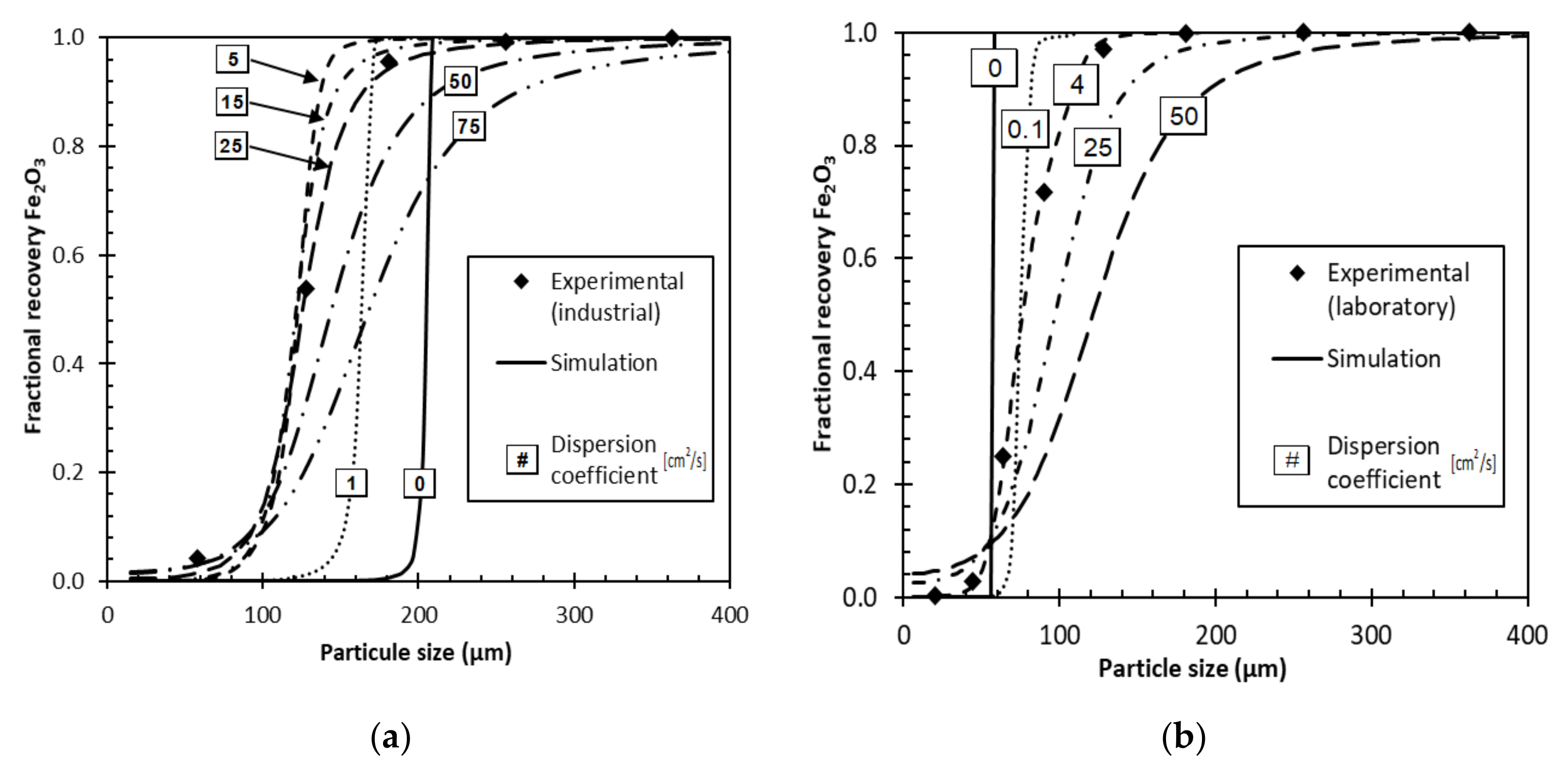
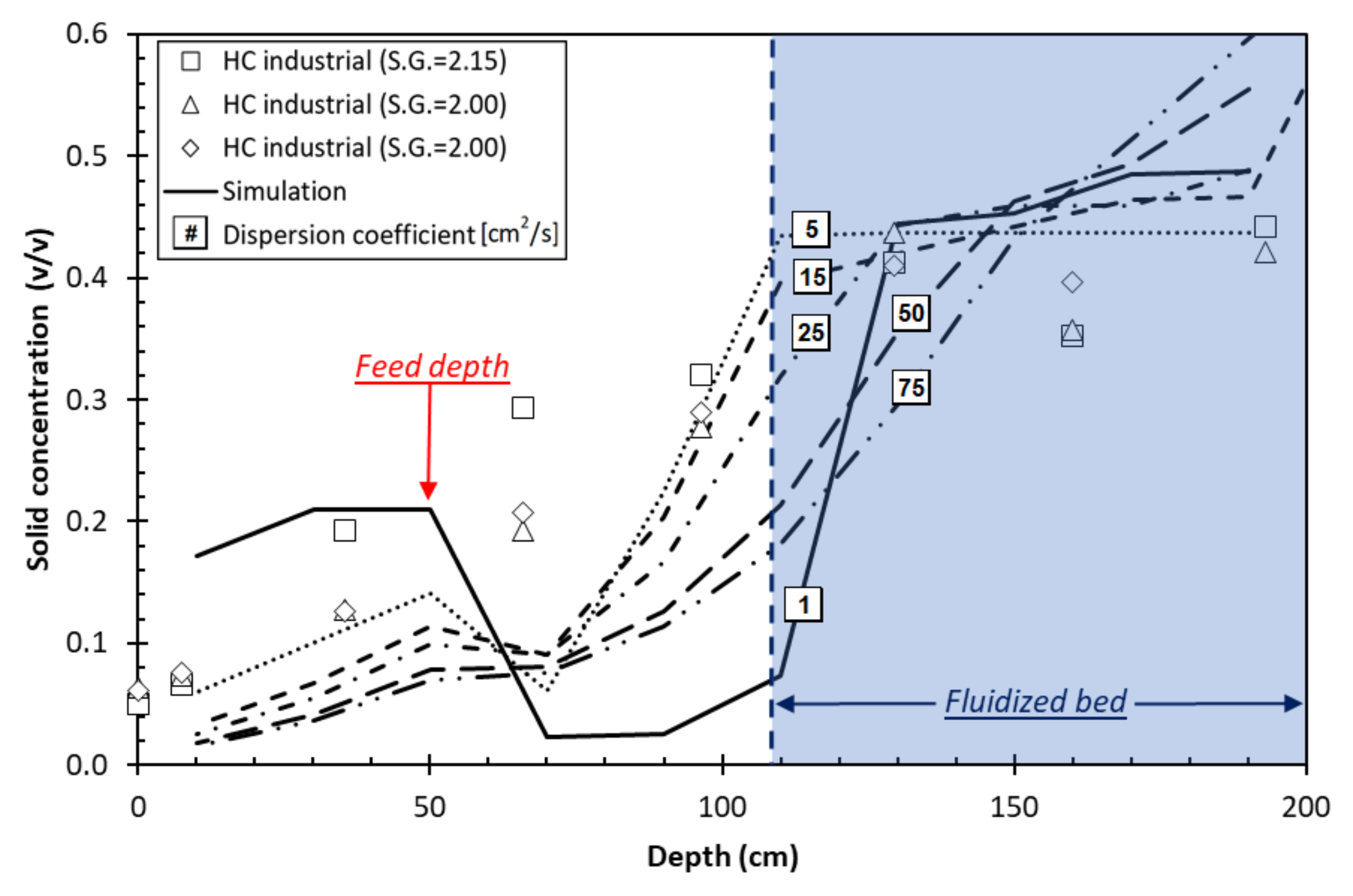
3.3.1. Dispersion Coefficient

Figure 4 shows the variation of the hematite partition curve as a function of D (axial dispersion coefficient) during the simulations of an experiment for the industrial (Figure 4a) and laboratory (Figure 4b) scales. These figures suggest that a value of D between 15–25 cm2/s yields the best fit for the industrial data, while a value of 4 cm2/s is more appropriate for the laboratory set-up. This latter value is very close to the 4–6 cm2/s reported by Kim [15]. The values obtained from the laboratory set-up also agree with the values found in the literature [18,19,20,21,22,29,30,31]. The higher D describing the industrial set-up is expectable because a larger back-mixing prevailing in the larger sizes as well as the flow rate of treated solid per unit area is larger in the industrial unit (e.g., ~10 m/h) compared to that of the laboratory one (~4 m/h). From the simulation results, a method for estimating D has been developed based on the value of the flow rate of treated solid per unit area. This method is presented in the work of Roy [24] and allows the simulation of the Hc when no experimental set-up is available.
Figure 5 shows the simulated axial profiles of the solid concentration for different values of D against the axial profiles’ concentration of the plant measured data. The feed element is located at 50 cm from the top of the Hc and the teeter injector at 200 cm from the top. Figure 5 confirms that a low D produces a variation in solid concentration as a function of depth that is not consistent with the observations made around the Hc feed zone. It also can be observed in Figure 5 that an increase in the value of D decreases the slope of the solid concentration around the feed but increases the slope of the solid concentration in the fluidized bed zone. The difference between simulation and observation could be due to the inclusion of the dispersion term ( D 2 C / z 2 in the computational algorithm to represent the pulp density re-equilibrium in the feed area due to Archimedes’ principle and that D is kept constant over the height of the Hc (Assumption 2).

3.3.2. Methods to Estimate the Porosity of the Fluidized Bed

The Hc can be divided into 6 zones according to the characteristics of the pulp flow [16]. This division is shown in Figure 6. The water added to the feed increases the upward velocity of the fluid in zones A, B and C. This velocity is different from that in zones D, E and F. The teeter water causes the same type of variation (fluid velocity) between zones D and E and the collection zone F. As a result, the velocity of the water in the classifier varies according to the height in the device. This is also valid for the solid concentration (Figure 1), which also varies along the height of the apparatus, implying a variation in the density and viscosity of the pulp.
The minimum porosity or maximum volume concentration of compaction of the ore (zone F, Figure 6), before the underflow, is estimated from the results of sampling campaigns showing that the solid concentration in the underflow is always in the vicinity of 47% v/v. If this value is adjusted to account for the fact that the cone water exits with the slurry in the underflow, then the volumetric solid concentration in zone F is 67%.
The bed porosity in zones D and E is estimated according to a minimum fluidization velocity analysis for multi-species and multi-sized solid-containing pulps similar to that of Asif and Ibrahim in 2002 [32]:
V m f ¯ r = k = 1 K X k V m f , k r
with V m f , k and X k which represent, respectively, the minimum fluidization velocity and the water-free solid volume fraction of species k . The exponent r can vary from 1 to 1 , thus passing from harmonic to arithmetic mean. Asif and Ibrahim [32,33] obtained better results with r = 1 , Rincon et al. [34] with r = 0.5 , while in the present analysis the best estimation of bed porosity was obtained with r = 1 .
To determine the value of the porosity of the fluidized bed, Equation (24) was used. The simulator calculates the arithmetic averaging particle velocity ( V m e a n , n φ ) as a function of total concentration ( φ ) over a range of values from 30% to 70%. From these results, the simulator considers the maximal concentration in bed of particles to be the one where the average velocity is closest to zero.
V n φ ¯ j = 1 J k = 1 K X j , k , n V j , k , n φ 0
where V j , k , n φ is the hindered settling velocity of particles of dimensions j of species k when the total concentration of the element is equal to φ .

4. Results and Discussion

4.1. Evaluation of the Calculation Algorithm

The simulation model will be validated with performance indices (Equation (A2), Appendix A.2) on a set of experimental data, including a total of 23 industrial experiments (1 to 23) and 8 laboratory experiments (L-1 to L-8). The experimental conditions are presented in Table 2 (and Figure A5 in Appendix C). Figure 7 shows the global underflow recovery of hematite (Fe2O3) and quartz (SiO2) for all experiments. The simulation model provides a good estimate of the experimental values. It also demonstrates that the simulation algorithm can be adapted to different flow regimes (laminar/turbulent) and Hc geometry (size and shape). Furthermore, the simulation algorithm remains stable despite the presence of a discontinuity in the solid concentration of the pulp as a function of depth. This stability comes from the addition of an analysis loop that separates the particle velocity caused by convection into two variables ( V j , k , V j , k ) depending on their direction (Equation (5)).

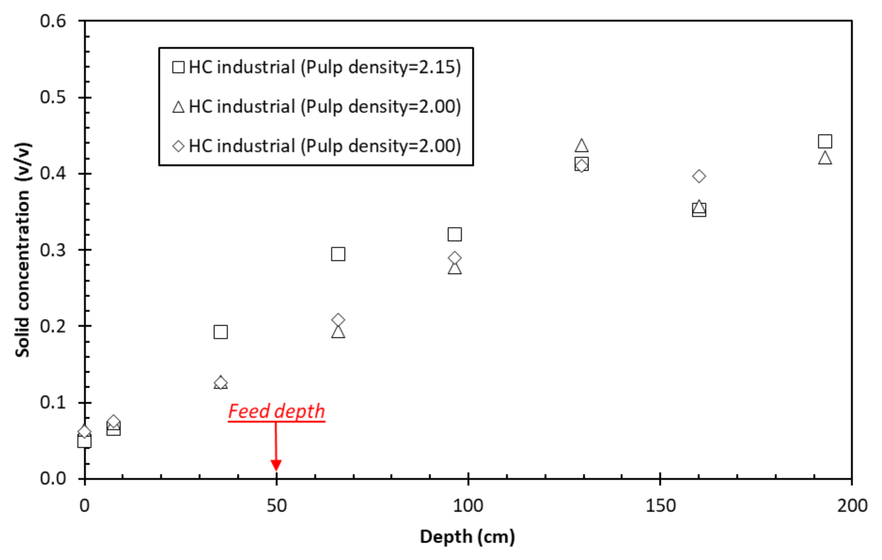
4.2. Influence of Pulp Density

Hcs as physical separation devices generate a dense particle bed that offer the exploitation of the gravitational force and the density differences between solid particles and their surrounding environment. This makes quartz particles (SiO2; specific gravity = 2.7) more dependent on the density variations of the pulp in zones D, E and F (Figure 6) than the hematite particles (Fe2O3; specific gravity = 5.2). However, the pulp density in these zones is not known as only the density of the slurry in the upper part of the Hc is measured, which includes zones A to D. Hence, lack of representation of the local density tends to inflate the error in simulating the behavior of light particles as their behavior in the pulp largely depends on the density of these zones.
Figure 8 shows the pulp density as a function of depth for three industrial-scale tests. Taken together, the experiments show that heavy particles behave significantly more predictably than light particles. This difficulty in adequately representing the displacement of light particles comes partly from the fact that the density of the pulp in the fluidized bed is close to the density of the quartz particles making all the particles of this species more dependent on the motion of medium then the dispersion force. Furthermore, as shown in Figure 5, the dispersion coefficient will be stronger in the feed zone than in the fluidized bed. Nevertheless, for simplicity, the dispersion coefficient has been assumed to be constant over the height of the apparatus (Assumption 2, Section 3.1). The dependence on the dispersion force of quartz makes its behavior slightly more difficult to predict.

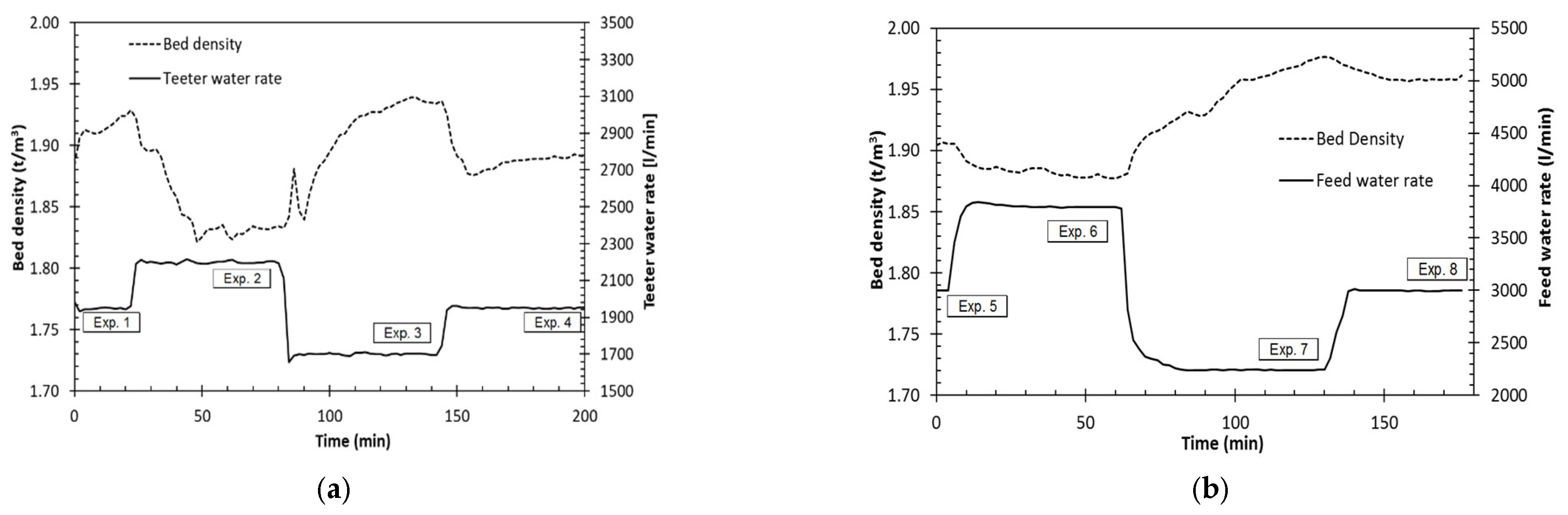
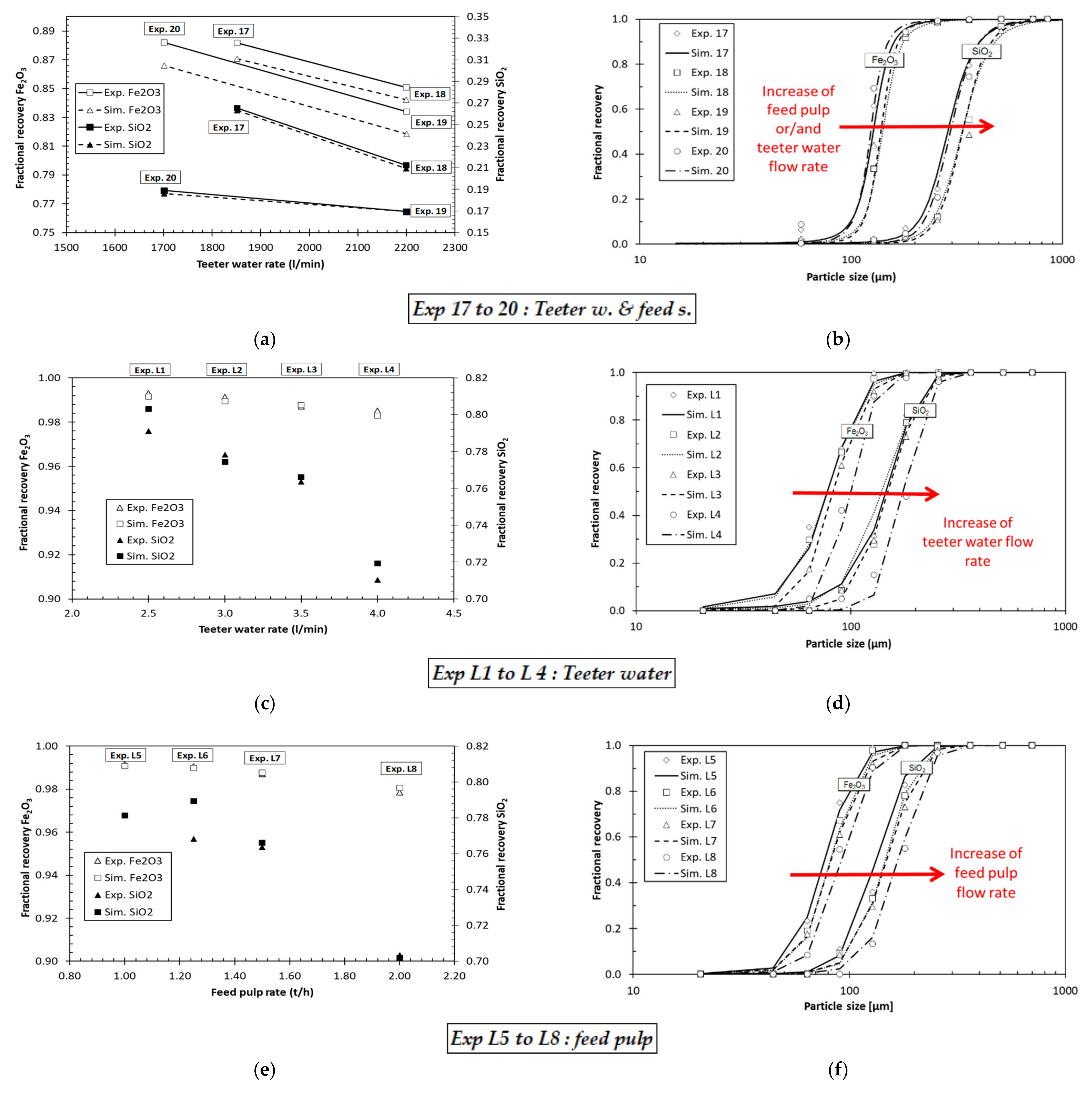
4.3. Control Variables

The two main operating variables used to control the operation of an Hc against the natural disturbances (iron oxide composition and size distribution) are:
  • The upper bed density as measured by a pressure sensor and manipulated via the opening of the Hc underflow valve;
  • The flow rate of teeter water flow rate that is used to correct an underflow composition (e.g., SiO2 content) that is off-spec.
Although these control variables are widely accepted as those that need to be manipulated to maintain a target operating performance for the Hc, it is somewhat surprising to find the void on the role of these variables in the literature dealing with the modeling of Hc. The proposed model provides a noise-free environment to study the impact of these variables on the performance of the Hc.
Figure 9 and Figure 10 show the values of the hematite and quartz weight recovery fraction at the Hcs underflow obtained experimentally and with the simulation model as a function of the different simulated operating variables, and as a function of the particle size. The figures show that to increase the underflow recovery, it is possible to decrease the flow of teeter water (experiments 1–4 and L1–L4); decrease the flow of feed water (experiments 5–8). When the unit is operated with a constant underflow valve opening value, it is possible to decrease the flow of the solids’ flow rate of the feed (experiments 9–12) or increase the opening of the underflow valve (experiments 13–16). While when controlling the bed density set point, it is necessary to increase the solids’ flow rate of the feed (experiments 17–20) or decrease the pulp density set point. The amount of light particle found in the underflow can be decreased by increasing the density of the pulp in the fluidized bed to inhibit the passage of light particles (experiments 5–8 and 13–16) or with decreasing the water flow rate at the top of the apparatus to reduce the loss of heavy particles in the overflow.
In summary, Figure 9 and Figure 10 show that the effect of the fluidization water is well captured by the simulator as well the effect of the bed density or valve opening, and this capability is used in [24] for studying control strategies that can reduce the variability reported in Figure 3 and as a way to define strategies to minimize iron losses while maintaining a low silica content in the Hc underflow.

4.4. Simulation of Primary, Secondary and Tertiary Hc

One of the objectives of the model development was to establish a mathematical model for the Hc that can be used to simulate an Hc without requiring calibration if the characteristics of the feed material change. The ability of the model to represent the operation of the primary Hc is demonstrated in Section 4.1, but whether this model could be used or not to predict the performances of secondary and tertiary Hcs (see Figure A2, Appendix A.2) remains to be checked. Finally, Table 3 gives the observed and simulated global performance indices for the primary, secondary and tertiary Hcs (see Figure A2, Appendix A.2). These results were obtained without altering calibration of the original model. The only input variables that were changed from one simulation to the other are the solid feed rate, the Hc feed mineral contents and the particle size distribution, and the dimensions (diameter and height) of the Hc. The Hc operating conditions (teeter water flow rate and bed density) applied for the simulation are those used in the plant. Despite the differences in the applications of the three Hcs, the model predictions are close to the Hc actual performances confirming that the fundamental approach used to develop the model ensures robustness and flexibility to simulate the behavior of various materials when processed in an Hc.

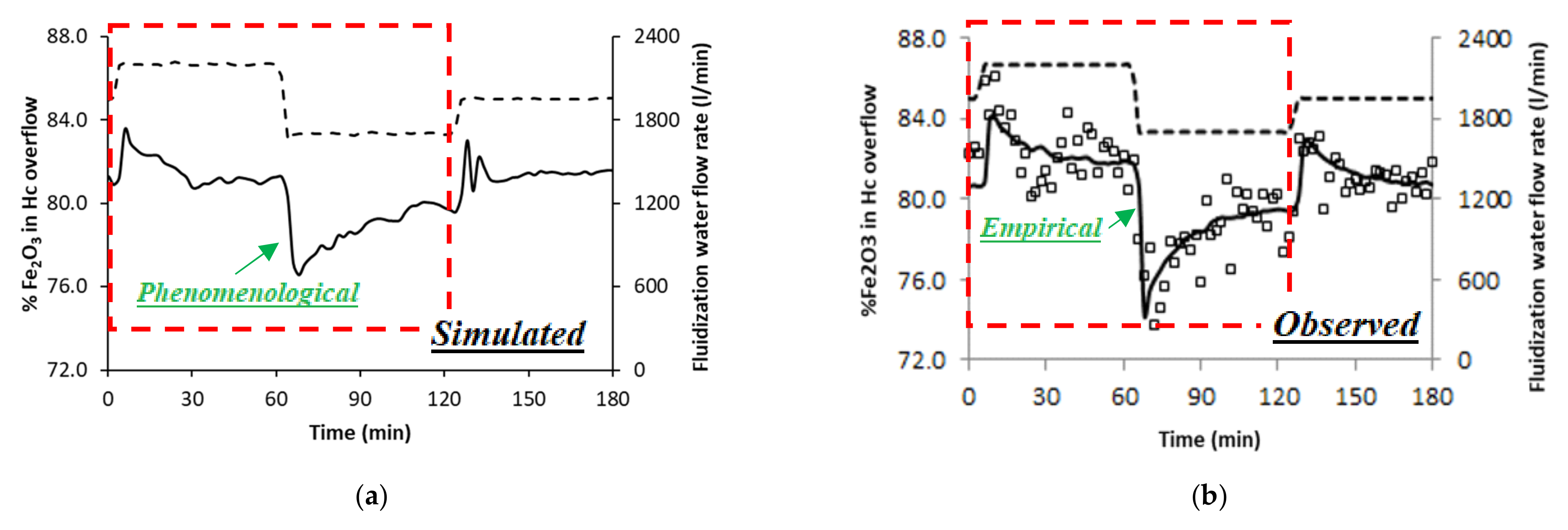
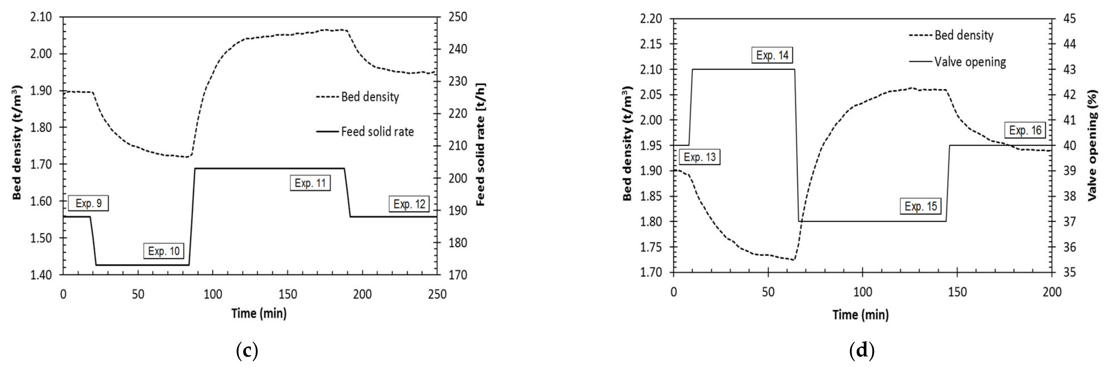
4.5. Dynamic Simulations

The model is built to allow the dynamic (time variation) simulation of the Hc response to step changes in the main Hc input variables. Details and other dynamic simulations can be found in [24]. An example of a dynamic simulation in response to step changes in the fluidization water flow rate is shown in Figure 11. This dynamic simulation example (Figure 11a) follows the same operating conditions as the industrial experiments 1 to 4 (Figure 11b). The iron oxide content in the Hc overflow is used as the output variable. The curve superimposed on the sampled values in Figure 11b was produced with an empirical simulation model proposed in the work of Payenzo [25], while that in Figure 11b was produced with the phenomenological simulation model presented in the present work. The simulated response is consistent with the observed response shown in Figure 11b where it can be seen that the simulator is able to predict the observed trend on the step response. This good prediction ability was possible without any adjustment to the calibrated model, confirming that the simulator could be used to virtually assess control strategies. Part of the observed error between the simulation and the experimental values comes from the fact that the experiments were carried out with a constant valve opening and that the simulation was carried out by modifying the underflow rate to follow the bed density obtained in these experiments. In addition, an error is contributed by the presence of particles that are not fully released and therefore have intermediate densities between heavy and light particles.

5. Conclusions

A one-dimensional dynamic model based on phenomenological convection/diffusion transport equations has been developed to simulate the operation of industrial Hc and of a laboratory for the separation of hematite from quartz. The model is able to predict both the steady state and dynamic responses of an industrial Hc to changes in teeter water addition and bed density.
The use of the assumptions presented in Section 3 allows to simplify the solution of the system of equations (Equations (2), (13), (21) and (22)) and allows to obtain the versatile simulation model. However, the study shows that assumption 2 is not always representative of the real behavior of the pulp (Section 3.3.1, Figure 5) and would require further investigation of the dispersion behavior as a function of depth under ranges of operating conditions similar to those of the experiments presented in Table 2.
In this research, it was possible to observe that the simulation of quartz is more subject to prediction errors than hematite. In addition to the error generated by the very low content of quartz in certain size classes and its non-uniform size distribution discussed in the work of Roy [24], it is possible to observe in Section 4.2 that the density of quartz is very close to the density of the fluidized bed, which increases the chances of error in the prediction of behavior and increases the influence of the dispersion at the expense of convection. Moreover, part of the error generated by the simulation model comes from the fact that the simulation algorithm does not take into account the particles that have not undergone a complete liberation, thus an intermediate density.
Nevertheless, the simulator has helped, for instance, to verify the following patterns and trends.
  • To increase the underflow recovery, it is possible to:
    • Decrease the flow of teeter water or feed water;
    • Increase the opening of the underflow valve or decrease the pulp density set point;
    • Decrease the solids flow rate of the feed with a constant underflow valve opening;
    • Increase the solids flow rate of the feed while maintaining a constant slurry feed pulp density.
  • To decrease the yield of light particle in the underflow, it is possible to increase the density of the pulp in the fluidized bed to help hinder their buildup in the underflow.
  • To decrease the loss of heavy particles in the overflow, it is possible by decreasing the water flow rate at the top of the apparatus without disturbing the fluidized bed under the feed by reducing the amount of water introduced by the feed (when it is allowed).
The simulation algorithm proves to be an asset to help in the choice of operating conditions by allowing the testing of various adjustments without disturbing the industrial process. The model is flexible as it allows the representation of variations in the partition curves of hematite and quartz for industrial and laboratory applications.

Author Contributions

J.R.: algorithm development, writing; F.L.: supervision of research, contribution to writing, review and editing; C.B.: supervision of research, project administration, funding acquisition, contribution to writing, review and editing. All of the authors contributed to analyzing the results and writing the paper. All authors have read and agreed to the published version of the manuscript.

Funding

This research was funded by ArcelorMittal and Mitacs Acceleration. The first author received a MITACS-Acceleration scholarships #IT 02457.

Data Availability Statement

Acknowledgments

Jonathan Roy thanks ArcelorMittal, Mitacs Acceleration and the University Laval for the support provided.

Conflicts of Interest

The authors declare no conflict of interest.

Abbreviations

aFeed/area
C Concentration (v/v)
dParticle diameter (m)
d 50 Median diameter (m)
DAxial dispersion coefficient (m2/s)
iTime interval
jParticle-size class
JMaterial mass flux (kg/s)
kSpecies
maxMaximum
nElement number/Richardson–Zaki index
NTotal number of elements
N f Feed element number
oOverflow
pPulp
QVolumetric flow (m3/s)
ReReynolds number
sSolid
tTime (s)
uUnderflow/free settling velocity (m/s)
UHindered settling velocity (m/s)
vVolume (m3)
VVelocity (m/s)
V m f Minimum fluidization velocity (m/s)
V Ascending velocity (m/s)
V Descending velocity (m/s)
wWater
XFluid-free volume fraction of solid
zHeight (m)
εPorosity
ρDensity (t/m3)
φTotal concentration

Appendix A

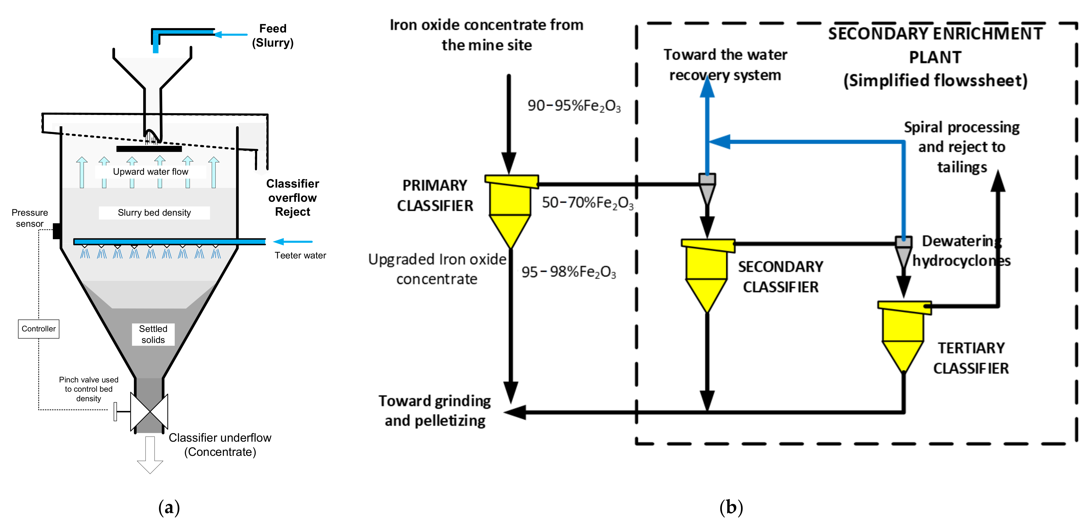
Appendix A.1. Hydraulic Classifiers (Hcs) for the Processing of Iron Ores

The data used for the development of the model were obtained by sampling industrial Hcs operated at the ArcelorMittal pellet plant in Port-Cartier (Canada) and by conducting tests using a laboratory set-up. The industrial and laboratory data were obtained from tests conducted using an iron oxide concentrate originating from the processing of the Mont-Wright mine iron ore (Canada). The iron ore extracted from the mine assays about 30% Fe in the form of hematite (Fe2O3; S.G. 5.2) in a gangue consisting mainly of quartz (SiO2; S.G. 2.7). The mined ore is transported to a nearby concentrator where it is crushed and ground down to less than 2 mm aiming at a liberation of the valuable (hematite) minerals from the non-valuable (quartz) minerals. The ground ore is then processed by spiral concentrators that separate the mineral particles on the basis of their densities [12]. The three consecutive stages of spiral concentration shown in Figure A1a are used to produce an iron oxide concentrate (IOxC) that assays 66% Fe (95% Fe2O3 and 5% SiO2). This IOxC is transported by train from the mine site to the pellet plant (about 300 km south) that prepares a portion of the concentrate for sale, as is, to steel producers. The other portion of the IOxC is prepared for specific customers that require a higher-grade product under the form of 1 cm diameter balls or pellets. Hcs are used to upgrade the IOxC from 95% Fe2O3 to 98% Fe2O3 by removing light silica minerals. The sequence of the steps from the mine to the production of enriched iron oxide pellets is shown in Figure A1b. The studied Hcs are operated at the pellet plant to increase the iron content of the IOxC by removing fine particles of quartz that are discarded to a tailings pond. In this special application, the Hcs are not located at the mine site. This is not a general practice as some iron ore concentrators [35] have started to incorporate Hcs within the iron ore spiral concentration circuit. This has stimulated interest on further improving the understanding of Hc operation.
Figure A1. ArcelorMittal mine, concentrator and pellet plants. (a) Iron ore processing from ore to the iron oxide products; Mine, concentrator and pellet plants. (b) Concentrator at the mine site; Production of the IOxC (mine and concentrator).
Minerals 12 00316 g0a1

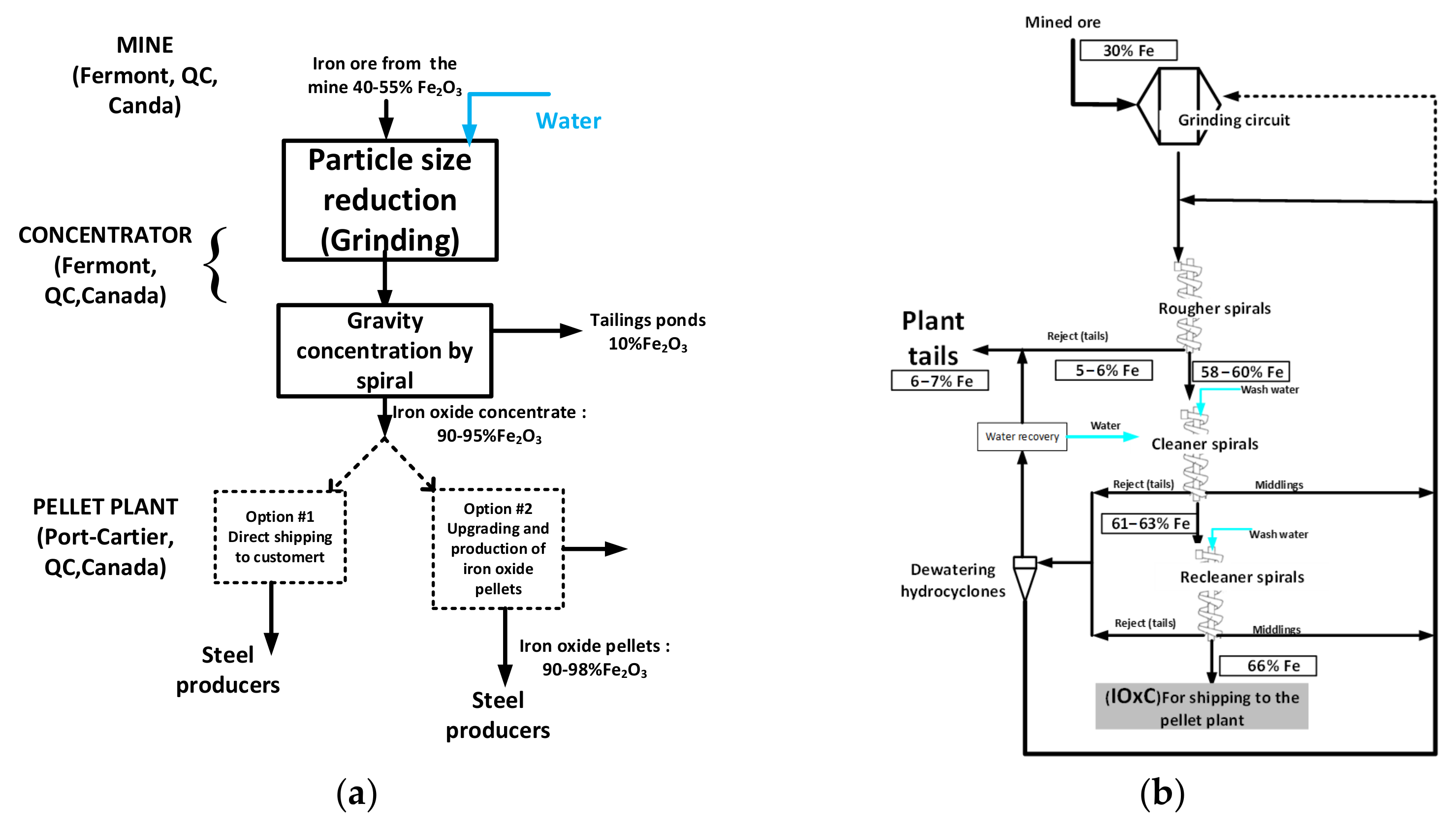
Appendix A.2. Operation of Hydraulic Classifiers for Upgrading Iron Oxide Concentrate at the ArcelorMittal Pellet Plant

The principle of operation of a hydraulic classifier is shown in Figure A2a. The feed is a slurry of water and particles and enters the top of the classifier. The slurry is then exposed to an upward flow of water that entrains the light particles (e.g., quartz) to an overflow launder while the heavy particles (e.g., coarse and medium size hematite) settle and are recovered at the bottom of the hydraulic classifier as an upgraded concentrate. Depending on the operating conditions, a portion of the fine heavy (valuable) minerals is lost to the classifier overflow. The operation of the Hc is controlled by:
  • The opening of the underflow valve that is used to adjust the density of the bed above the injection of teeter water;
  • The flow rate of teeter or fluidization water (see Figure A2a).
The upgraded iron oxide is recovered as the Hc underflow while the classifier overflow contains the rejected quartz but also some valuable iron oxide minerals that it is worthy to recover, as will be discussed later. The ArcelorMittal pellet plant operates Hcs for different purposes as shown in Figure A2b. Details of the process used by ArcelorMittal in the concentrator and pellet plant are presented in several papers [5,6,12,24,25,36]. The main application is the upgrading of the IOxC. Indeed, the primary Hcs are designed to process more than 200 t/h of concentrate delivered from the mine site. Since the upgrading process causes a loss of valuable iron oxide through the hydraulic classifier overflow (see Figure A2a), the primary classifier overflow stream is directed toward a secondary Hc (Figure A2b) that is operated to recover the iron oxide lost from the primary classifier. As for the primary Hc, the separation between iron oxide and quartz being imperfect, the overflow from the secondary Hc still contains valuable iron oxide and is thus directed toward a tertiary Hc whose role is to recover the lost iron oxide from the secondary classifier. The characteristics of the feed material are different for the primary, secondary and tertiary Hc; the hydraulic classifier model thus should be successful in simulating the three cases as a demonstration of its robustness.
Figure A2. Simplified diagrams of the (a) hydraulic classifier and (b) primary upgrading of the IOxC.
Minerals 12 00316 g0a2

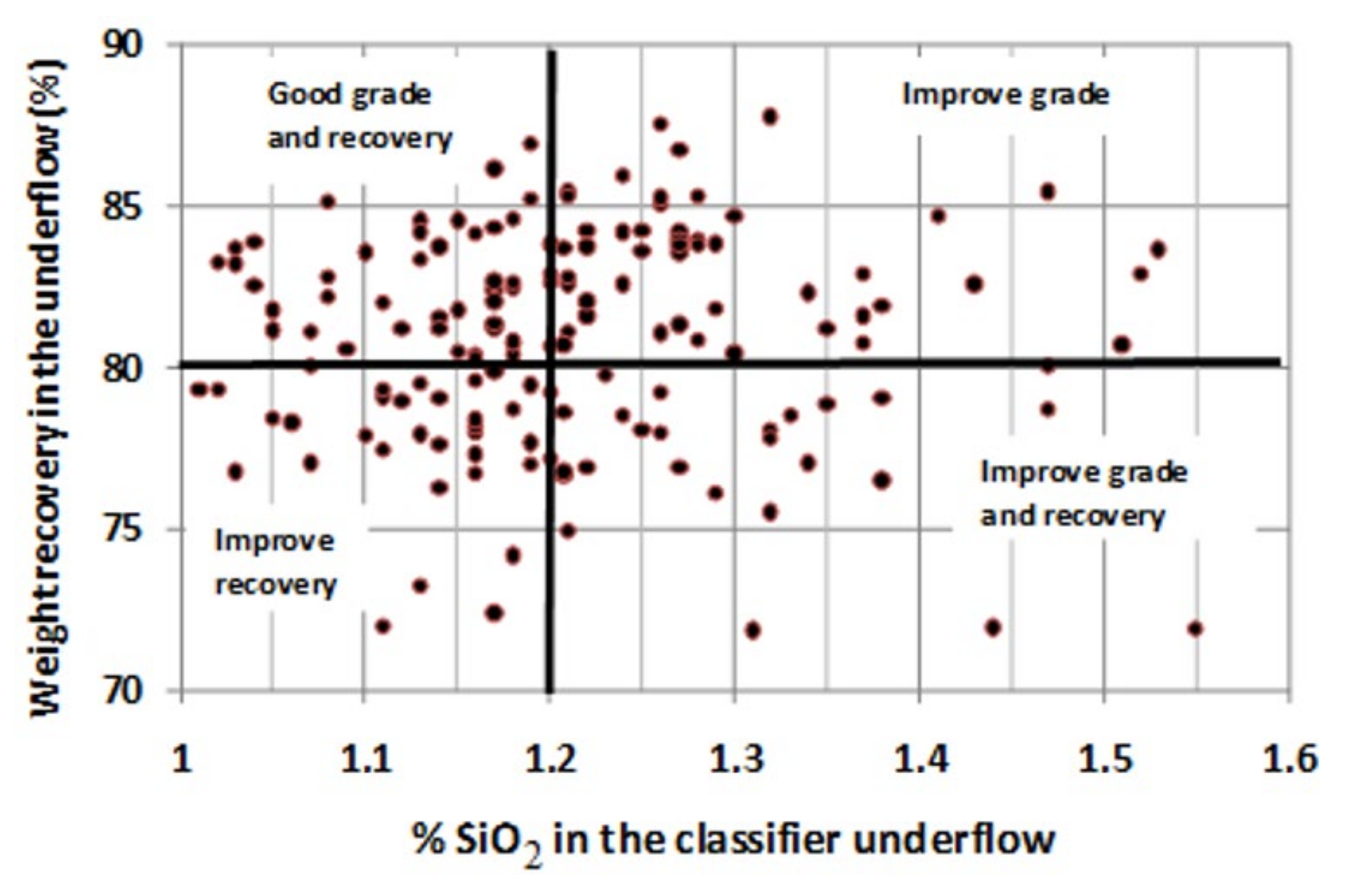
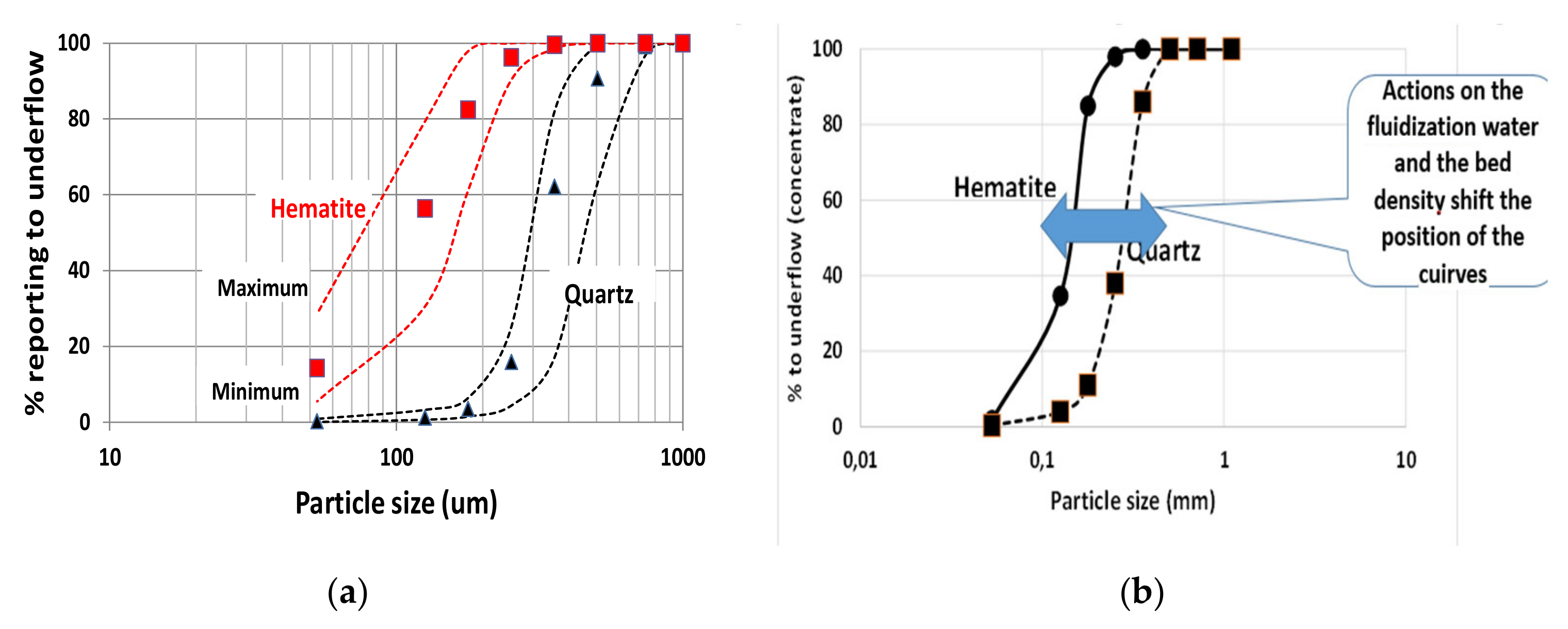
Appendix A.3. Performance Indices for the Hydraulic Classifier

The performance of an Hc is monitored using the weight recovery to the underflow and its silica content. The weight recovery to the underflow is given by:
R U = W u W F
where W stands for the solids’ flow rates in the Hc and the subscripts F and u represent the feed and underflow streams. Figure A3 shows the observed variations of the weight recovery and silica content of the underflow over a period of 200 days on stream. The dispersion of the performance indices about the plant targets of 80% weight recovery at 1.2% SiO2 in the upgraded concentrate shows room for improvement that process control could help to achieve. Such aim can only be achieved if the effect of the manipulated variables on the performance indices are well understood, a knowledge that a mathematical model can help to acquire. The reasons for the discrepancy between the indices presented in Figure A3 and the plant objectives are multiple. However, it is possible to conclude that they are mostly due to the lack of knowledge of the influence of variations in granulometry and feed grade on the efficiency of the separation process. The operating parameters are therefore constantly adjusted when the disturbance is observed on the performance variables.
The weight recovery and the silica content of the upgraded concentrate are global performance indices that, although well accepted by the operators, do not inform about the phenomena occurring within the Hc. A better insight into the way the heavy (hematite) and light (quartz) minerals are separated within the classifier is provided by the partition curves of the minerals. The partition factor of a mineral gives the proportion of a mineral within a size interval of the feed stream that is recovered in the classifier underflow. The partition factor for mineral k within size interval j ( R j , k ) is given by:
R j , k = w j , u x j , k , u w j , f x j , k , f ,
where w   and x are the are the weight fractions of solids and mineral concentration, while the the subscripts j and k represent the size interval and the specie. The graph of the partition factors as a function of particle size gives the partition curves for the minerals in the classifier. The average partition curves for hematite and quartz obtained from seven sampling campaigns conducted on the primary hydraulic classifiers of the ArcelorMittal pellet plant are shown in Figure A4a. The method to obtain these curves is presented in the Section 2.1 and in the work of Roy [24]. Results of Figure A4a show that on average 50% of the hematite particles coarser than 0.1 mm (100 µm) report to the underflow, while this proportion is less than 5% for quartz of the same size, thus explaining the origin of the upgrading process occurring in the Hc.
Figure A3. Weight recovery and silica content of the classifier underflow observed for 200 on-stream days of operation [6].
Minerals 12 00316 g0a3
The Hc operators can adjust the flow rate of teeter water and the bed density to shift the mineral partition curves (see Figure A4b) and thus modify the global performances (weight recovery and %SiO2 of the upgraded concentrate) of the classifier. Despite the numerous experiments conducted in the plant, it was not possible to experimentally identify the effect of these operating variables on the mineral partition curves [6]. Therefore, the model described in this work will provide, for the first time, a way to discriminate between the effects of these operating variables on the partition curves.
Figure A4. Simplified diagrams of the (a) partition curves for hematite and quartz in the primary Hcs of Figure A3 and (b) the position of the partition curves can be changed by acting on the fluidization water and thus on the bed density. Symbols are the average values of 7 sampling campaigns; dashed lines give the extreme values observed.
Minerals 12 00316 g0a4

Appendix B

Several equations have been developed to estimate the hindered-settling velocity ( U j , k , n ) of the particles. The equations developed by Hartman et al. [26] allow to estimate directly, without iterative calculation, the sedimentation velocity of a single particle u j , k :
A r j , k = ρ e g d j 3 ρ k ρ e μ e 2 ,
A j , k   = l o g 10 A r j , k ,
R a j , k = 0.99947 + 0.1848 sin 1.848 A j , k 3.14 ,
P a j , k = 0.0017795 A j , k 0.0573 A j , k + 1.0315 A j , k 1.2622 ,
l o g 10 R e k t i = P a j , k + l o g 10 R a j , k ,
R e j , k = 10 P a j , k + l o g 10 R a j , k ,
u j , k = R e j , k μ e ρ e d j .
Several empirical equations have also been proposed to determine the sedimentation rate of particles in a dense medium (hindered settling) [7,27,28,37,38]. The model proposed by Patwardhan and Tien [39] to predict the slip velocity considers the terminal sedimentation velocity in water, the interparticle distance and the suspension density:
U j , k = u j , k · F ε · G ρ
where U j , k is the hindered terminal sedimentation velocity in pulp, u j , k is the terminal sedimentation velocity in water, F ε takes into account the interparticle distance and G ρ is related to the density difference between the particles and the surrounding fluid. Masliyah [27] proposes the following equations to estimate, F ε and G ρ :
F ε = ε n 2 ,
G ρ = ρ k ρ p ρ k ρ f .
The density indices k , f and p designate, respectively, the solid, the fluid and the pulp, and ε is the bed void fraction. The variable n depends on the Reynolds number and varies with particle size and density. The method of Rowe [28] is used to determine the Richardson and Zaki index n as follows:
n = 2 2.35 + 0.1175 R e 0.75 1 + 0.175 R e 0.75 .

Appendix C

Figure A5. Bed density and manipulated variable as a function of time for industrial experiments (a) 1 to 4; (b) 5 to 8; (c) 9 to 12; (d) 13 to 16.
Minerals 12 00316 g0a5aMinerals 12 00316 g0a5b

References

  1. Wills, A.B.; Finch, A.J. An Introduction to the Practical Aspect of Ore Treatment and Mineral Recovery; Elsevier: Amsterdam, The Netherlands, 2015. [Google Scholar]
  2. Burt, R.O. The role gravity concentration in modern processing plants. Miner. Eng. 1999, 12, 1291–1300. [Google Scholar] [CrossRef]
  3. Das, A.; Sarkar, B. Advanced gravity concentration of fine particules. Miner. Process. Extr. Metall. Rev. 2018, 39, 359–394. [Google Scholar] [CrossRef]
  4. Tripathy, S.K.; Bhoja, S.K.; Kumar, C.R.; Suresh, N. A short review on hydraulic classification and its development in mineral industry. Powder Technol. 2015, 270, 205–220. [Google Scholar] [CrossRef]
  5. Bazin, C.; Payenzo, G.M. Analysis and modelling of the operation of a hydraulic classifier for iron ore concentrate. In Proceedings of the Physical Separation: Mineral Engineering Conference, Falmouth, UK, 5–8 May 2011. [Google Scholar]
  6. Bazin, C.; Payenzo, G.M.; Desnoyers, M.; Gosselin, C.; Chevalier, G. The use of simulation for process diagnosis: Application to a gravity separator. Int. J. Miner. Process. 2012, 104, 11–16. [Google Scholar] [CrossRef]
  7. Sarkar, B.; Das, A. A comparative study of slip velocity models for the prediction of performance of floatex density separator. Int. J. Miner. Process. 2010, 94, 20–27. [Google Scholar] [CrossRef]
  8. Das, A.; Sarkar, B.; Mehrotra, S.P. Prediction of separation performance of Floatex Density Separator for processing of fine coal particles. Int. J. Miner. Process. 2009, 91, 41–49. [Google Scholar] [CrossRef]
  9. Das, A.; Sarkar, B.; Biswas, P.; Roy, S. Performance prediction of floatex density separator in processing iron ore fines—A relative velocity approach. Miner. Process. Extr. Met. 2009, 118, 78–84. [Google Scholar] [CrossRef]
  10. Sarkar, B.; Das, A.; Mehrotra, S. Study of separation features in floatex density separator for cleaning fine coal. Int. J. Miner. Process. 2008, 86, 40–49. [Google Scholar] [CrossRef]
  11. Sah, R.; Vidyadhar, A.; Das, A. Study of cut point density and process performance of Floatex density separator in fine coal cleaning. Part. Sci. Technol. 2017, 35, 239–246. [Google Scholar] [CrossRef]
  12. Sadeghi, M.; Bazin, C. The Use of Process Analysis and Simulation to Identify Paths to Improve the Operation of an Iron Ore Gravity Concentration Circuit. Adv. Chem. Eng. Sci. 2020, 10, 149–170. [Google Scholar] [CrossRef]
  13. Luttrell, G.H.; Honaker, R.Q.; Bratton, R.C.; Westerfield, T.C.; Kohmuench, J.N. Plant Testing of High-Efficiency Hydraulic Separators; Virginia Polytechnic Institue & State University: Blacksburg, VA, USA, 2006. [Google Scholar]
  14. Galvin, K.; Pratten, S.; Nicol, S. Dense medium separation using a teetered bed separator. Miner. Eng. 1999, 12, 1059–1081. [Google Scholar] [CrossRef]
  15. Kim, B.H. Modeling of Hindered-Settling Column Separations. Ph.D. Thesis, The Pennsylvania State University, State College, PA, USA, 2003. [Google Scholar]
  16. Honaker, R.Q.; Mondal, K. Dynamic modelling of fine coal separation in hindered-bed classifier. Coal Prep. 2000, 21, 211–232. [Google Scholar] [CrossRef]
  17. Cho, H.; Klima, S.K. Application of batch hindered-settling model to dense-medium separations. Coal Perp. 1994, 14, 167–184. [Google Scholar] [CrossRef]
  18. Syed, N.; Dickinson, J.; Galvin, K.; Moreno-Atanasio, R. Continuous, dynamic and steady state simulation of the reflux classifier using a segregation-dispersion model. Miner. Eng. 2018, 115, 53–67. [Google Scholar] [CrossRef]
  19. Asif, M. Modeling of multi-solid liquid fluidized bed. Chem. Eng. Technol. 1997, 20, 485–490. [Google Scholar] [CrossRef]
  20. Patel, B.K.; Ramirez, W.F.; Galvin, K. A generalized segregation and dispersion model for liquid-fluidized beds. Chem. Eng. Sci. 2008, 63, 1415–1427. [Google Scholar] [CrossRef]
  21. Kennedy, S.C.; Bretton, R.H. Axial dispersion of spheres fluidized with liquids. AIChE J. 1966, 12, 24–30. [Google Scholar] [CrossRef]
  22. Syed, N.H.; Khan, N.A.; Ahmad, I. A computational study of a multi-solid–liquid fluidized bed incorporating inclined channels. Chem. Ind. Chem. Eng. Q. 2021, 27, 223–230. [Google Scholar] [CrossRef]
  23. Lee, C.H. Modeling of Batch Hindered Settling. Ph.D. Thesis, The Pennsylvania State University, State College, PA, USA, 1989. [Google Scholar]
  24. Roy, J.; Bazin, C.; Larachi, F. Modélisation D’un Classificateur Hydraulique Pour l’Enrichissement d’un Concentré d’Oxyde de Fer. Ph.D. Thesis, Université Laval, Québec, QC, Canada, 2021. [Google Scholar]
  25. Mfudi, P.G. Modélisation d’un Classificateur Hydraulique à l’Usine de Boulettage d’ArcelorMittal. Master’s Thesis, Université Laval, Québec, QC, Canada, 2013. [Google Scholar]
  26. Hartman, M.; Havlin, V.; Tronka, O.; Carsky, M. Predicting the free-fall velocities of spheres. Chem. Eng. Sci. 1989, 44, 1743–1745. [Google Scholar] [CrossRef]
  27. Masliyah, J.H. Hindered settling in a multi-species particle system. Chem. Eng. Sci. 1979, 34, 1166–1168. [Google Scholar] [CrossRef]
  28. Rowe, P.A. Convenient emperical equation for estimatio of the Richardson-Zaki exponent. Chem. Eng. Sci. 1987, 42, 2795–2796. [Google Scholar] [CrossRef]
  29. Juma, A.; Richardson, J. Segregation and mixing in liquid fluidized beds. Chem. Eng. Sci. 1983, 38, 955–967. [Google Scholar] [CrossRef]
  30. Asif, M. Segregation velocity model for fluidized suspension of binary mixture of particles. Chem. Eng. Process. Process. Intensif. 1998, 37, 279–286. [Google Scholar] [CrossRef]
  31. Galvin, K.; Callen, A.; Zhou, J.; Doroodchi, E. Performance of the reflux classifier for gravity separation at full scale. Miner. Eng. 2005, 18, 19–24. [Google Scholar] [CrossRef]
  32. Asif, M.; Ibrahim, A.A. Minimum fluidization velocity and defluidization behavior of binary-solid liquid-fluidized beds. Powder Technol. 2002, 126, 241–254. [Google Scholar] [CrossRef]
  33. Asif, M. Predicting minimum fluidization velocities of multi-component solid mixtures. Particuology 2013, 11, 309–316. [Google Scholar] [CrossRef]
  34. Rincon, J.; Guardiola, J.; Romerero, A.; Ramos, G. Predicting the minimum fluidization velocity of multicomponent systems. J. Chem. Eng. Jpn. 1994, 27, 177–181. [Google Scholar] [CrossRef] [Green Version]
  35. Lavoie, F. Bloom Lake Flowsheet Assessment, One Year into Operation. In Proceedings of the CIM General Meeting, Montreal, QC, Canada, 11–16 May 2019; pp. 1–14. [Google Scholar]
  36. Hallab, S.; Poulin, É.; Hodouin, D. Modeling of a concentration plant to improve the carbon content control of iron oxide pellets. IFAC Proc. Vol. 2013, 46, 1–6. [Google Scholar] [CrossRef]
  37. Littler, A. Automatic hindered-settling classifier for hydraulic sizing and mineral beneficiation. Inst. Min. Metall. 1986, 95, 133–138. [Google Scholar]
  38. Garside, J.; Al-Dibouni, M.R. Velocity-Voidage relationships for fluidization and sedimentation in solid-liquid systems. Ind. Eng. Chem. Process Des. Dev. 1976, 16, 206–214. [Google Scholar] [CrossRef]
  39. Patwardhan, V.S.; Tien, C. Sedimentation and liquid fluidization of solid particles of different sizes and densities. Chem. Eng. Sci. 1985, 40, 1051–1060. [Google Scholar] [CrossRef]
Figure 1. Concentration of solids as a function of depth for industrial experiments.
Minerals 12 00316 g001
Figure 2. Elements of hydraulic classifiers.
Minerals 12 00316 g002
Figure 3. Zones of hydraulic classifies.
Minerals 12 00316 g003
Figure 4. Influence of the axial dispersion coefficient on the fractional recovery of hematite (Fe2O3) in the simulation of (a) an industrial experiment and (b) a laboratory experiment.
Minerals 12 00316 g004
Figure 5. Influence of D on the solid concentration in the simulation of an industrial experiment.
Minerals 12 00316 g005
Figure 6. The zones in a hydraulic classifier.
Minerals 12 00316 g006
Figure 7. Recovery in underflow: (a) for experiments 1 to 23 (industrial) and (b) for experiments L1 to L8 (laboratory).
Minerals 12 00316 g007
Figure 8. Experimental and simulated slurry pulp density as a function of depth.
Minerals 12 00316 g008
Figure 9. Fractional recovery of Fe2O3, SiO2 in underflow as a function of (a,b) teeter water rate (exp. 1–4), (c,d) feed water rate (exp. 5–8), (e,f) feed solid rate (exp. 9–12) and (g,h) valve opening (exp. 13–16); exp: experiment.
Minerals 12 00316 g009
Figure 10. Fractional recovery of Fe2O3, SiO2 in underflow as a function of; (a,b) teeter water and feed pulp rates (exp. 17–20), (c,d) teeter water rate (exp. L1–L4) and (e,f) feed pulp rate (exp. L5–L8); exp: experiment.
Minerals 12 00316 g010
Figure 11. Recovery of Fe2O3 in overflow as a function of teeter water for experiments 1 to 4: (a) simulated and (b) observed.
Minerals 12 00316 g011
Table 1. Operating conditions of experiments on industrial and laboratory set-ups.
CharacteristicsUnitsType of Hc
LaboratoryIndustrials
PrimarySecondaryTertiary
Heightm1.5444
Widthm0.062.132.133.15
Aream20.0034.54.57.8
Shape-CircularSquareSquareCircular
Bed densityt/m31.1–1.41.7–2.21.7–1.81.7–1.8
Teeter waterl/min1–2~2000~1000~1000
Feed (solid)t/h0.05–0.1150–30080–10090–110
Feed (water)l/min~43000–4000~2000~4000
Table 2. Operating conditions of experiments on industrial, and laboratory set-ups.
TestTypeSolidWaterTeeterWaterPulp
Feed RateFeed RateWaterConeDensity
[t/h][L/min][L/min][L/min][t/m3]
1Indutrial188299819482501.92
2Ind.188300421912501.85
3Ind.187299717122501.91
4Ind.188300219432501.89
5Ind.188300019502501.91
6Ind.188376119502501.88
7Ind.188233419502501.94
8Ind.188289119502501.96
9Ind.188300319492501.9
10Ind.173299819492501.76
11Ind.203300119502502.01
12Ind.188300219502501.97
13Ind.188300319492501.89
14Ind.188300219502501.77
15Ind.188299819502502
16Ind.188299819502501.96
17Ind.171296118512032
18Ind.171298021992012
19Ind.144251022001882
20Ind.144250917011862
21Ind.265467220242502
22Ind.90234010002371.77
23Ind.10240009602501.77
L1Laboratory0.072.71.50.51.27
L2Lab.0.0731.50.51.33
L3Lab.0.073.61.50.51.35
L4Lab.0.0741.50.51.41
L5Lab.0.073.510.51.43
L6Lab.0.073.51.250.51.4
L7Lab.0.073.61.50.51.35
L8Lab.0.073.520.51.32
Table 3. Observed and simulated performance indices for the primary, secondary and tertiary Hcs of the ArcelorMittal pellet plant.
HcTestSolidWaterTeeterWaterPulpWeight Recovery (%)% SiO2 in Hc Underflow
FeedFeed RateWaterConeDensityHematiteQuartz
#[t/h][L/min][L/min][L/min][t/m3]Obs.Sim.Obs.Sim.Obs.Sim.
Primary21265467220242502.0083.783.035.235.02.12.1
Secondary2290234010002371.7725.626.91.93.62.64.5
tertiary2310240009602501.7740.043.92.31.43.01.7
Publisher’s Note: MDPI stays neutral with regard to jurisdictional claims in published maps and institutional affiliations.

