Article

3D Mineral Prospectivity Mapping of Zaozigou Gold Deposit, West Qinling, China: Machine Learning-Based Mineral Prediction

1
Geomathematics Key Laboratory of Sichuan Province, Chengdu University of Technology, Chengdu 610059, China
2
Key Laboratory of Geochemical Exploration, Institute of Geophysical and Geochemical Exploration, CAGS, Langfang 065000, China
3
Institute of Mineral Resources, Chinese Academy of Geological Sciences, Beijing 100037, China
*
Author to whom correspondence should be addressed.
Minerals 2022, 12(11), 1361; https://doi.org/10.3390/min12111361
Submission received: 31 July 2022 / Revised: 6 October 2022 / Accepted: 16 October 2022 / Published: 26 October 2022
(This article belongs to the Special Issue 3D/4D Geological Modeling for Mineral Exploration)

Abstract

:
This paper focuses on researching the scientific problem of deep extraction and inference of favorable geological and geochemical information about mineralization at depth, based on which a deep mineral resources prediction model is established and machine learning approaches are used to carry out deep quantitative mineral resources prediction. The main contents include: (i) discussing the method of 3D geochemical anomaly extraction under the multi-fractal content-volume (C-V) models, extracting the 12 element anomalies and constructing a 3D geochemical anomaly data volume model for laying the data foundation for researching geochemical element distribution and association; (ii) extracting the element association characteristics of primary geochemical halos and inferring deep metallogenic factors based on compositional data analysis (CoDA), including quantitatively extracting the geochemical element associations corresponding to ore-bearing structures (Sb-Hg) based on a data-driven CoDA framework, quantitatively identifying the front halo element association (As-Sb-Hg), near-ore halo element association (Au-Ag-Cu-Pb-Zn) and tail halo element association (W-Mo-Co-Bi), which provide quantitative indicators for the primary haloes’ structural analysis at depth; (iii) establishing a deep geological and geochemical mineral resources prediction model, which is constructed by five quantitative mineralization indicators as input variables: fracture buffer zone, element association (Sb-Hg) of ore-bearing structures, metallogenic element Au anomaly, near-ore halo element association Au-Ag-Cu-Pb-Zn and the ratio of front halo to tail halo (As-Sb-Hg)/(W-Mo-Bi); and (iv) three-dimensional MPM based on the maximum entropy model (MaxEnt) and Gaussian mixture model (GMM), and delineating exploration targets at depth. The results show that the C-V model can identify the geological element distribution and the CoDA method can extract geochemical element associations in 3D space reliably, and the machine learning methods of MaxEnt and GMM have high performance in 3D MPM.

1. Introduction

The main task of quantitative mineral prediction is to conduct comprehensive analysis of geological, geophysical, geochemical and remote sensing data and drilling engineering data in the study area based on the research of the geological background and metallogenic regularity, and then construct mathematical models to effectively extract and identify favorable information on mineralization, carry out data fusion of quantitative mineralization information, construct mineral prediction models, perform potential mineral resources quantitative assessment and exploration targets delineation [1,2,3].
Quantitative mineral resource prediction is developing toward deep 3D quantitative prediction. The framework of 3D quantitative mineral prediction has been basically completed, among which the representative works include Xiao [4,5,6,7,8,9,10], who studied the characteristics of large-scale three-dimensional mineralization prediction and summarized the combined prediction process of mine concession structure, mineral exploration model, metallogenic series and quantitative analysis methods, which laid the foundation for three-dimensional mineral resource prediction; Chen [11,12,13,14] proposed the “cubic prediction model” for mineralization prediction by 3D-comprehensive 3D modeling of geology, geophysics, geochemistry and remote sensing [15,16,17]; Mao [18,19,20,21,22] proposed a three-dimensional prediction process for deep mineral resources prediction, the three-dimensional morphological analysis of geological bodies, geological anomaly extraction and three-dimensional quantitative prediction methods [23]; Yuan [24,25] proposed a “four-step” three-dimensional mineralization prediction method, which summarizes the three-dimensional mineralization prediction work into four key steps: three-dimensional geological database construction, three-dimensional geological modeling and mapping, three-dimensional prediction information deep mining and three-dimensional geosciences data fusion and prediction.
In this study, three-dimensional quantitative mineral resources prediction is executed from a geological and geochemical perspective. It is a common understanding in the last century that the distribution of rock geochemical elements follows normal or lognormal distribution, based on which classical statistical theories and methods have been widely applied in the field of geochemical data analysis [26]. Since the 1990s, fractal and multifractal methods have been developed rapidly, with representative achievement from Cheng’s team, who proposed the content-area (C-A) model [26,27], the spectrum-area (S-A) model [28] and Local Singularity Analysis (LSA) [26,29,30,31,32], and it is believed that the multifractal distribution has the ability to simultaneously portray the normal distribution, lognormal distribution, Zipf’s law, Pareto’s law, etc., and can be used as the basic law of geochemical element distribution [26,29]. Based on the theoretical research of fractal and multifractal methods, its application in geochemical spatial distribution pattern research is blossoming [10,33,34,35,36,37]. The multifractal-related methods have achieved many successful cases in regional geochemical anomaly extraction [32,38,39,40,41,42,43,44,45]. With the improvement of 3D software and hardware performance, as well as the development of 3D modeling technology, fractal models used in 3D data have made some progress [34,46,47]. Three-dimensional primary halo geochemical survey is an effective tool for deep mineral resources prediction. In fact, the spatial zonation pattern of primary haloes is the pattern of element clustering regularity in 3D space, and the anomalous structure of elements is an intuitive indicator of deep mineral prediction. Especially, Cheng [27] proposed that the distribution of geochemical elements in either horizontal or vertical directions is consistent with the fractal distribution, based on which Afzal [34] proposed the C-V model, which is a powerful tool to delineate the nonlinear characteristics of element distribution in a 3D space.
Geochemical data are typically compositional data, which gives rise to the problem of “closure effects” due to the lack of scale consistency in the covariance matrix of the compositional data [48,49,50], and, in practice, classical geostatistical methods that ignore the compositional properties of geochemical data often yield poor results [51,52,53,54,55,56,57,58,59,60]. Since the introduction of Aitchison geometry and the application of additive log-ratio transformation (alr) [61], the theory and methods of log-ratio transformation of compositional data have been gradually improved, making the application of classical statistical methods more reasonable [33,35]. The geochemical elemental association extraction method based on Sequential Binary Partition (SBP) [50] can design elemental associations based on the geological background and mineralization knowledge, which is easy to interpret, and provides solutions for geochemical inference of lithology, tectonics, alteration, mineralization, etc. Therefore, the CoDA method provides new ideas for analyzing the relationship of geochemical data and extracts geochemical associations for evaluating mineral resources rapidly [51,55,62,63,64,65,66,67].
Geosciences is a data-intensive science, and geological survey and mineral exploration have accumulated a large amount of multi-source geosciences data, and the introduction of big data and its application of machine learning-related methods can effectively support mineral resources exploration [26,68,69,70,71,72,73]. During the past decade or so, a large number of achievements related to machine learning have been published in geosciences [37,57,74,75,76,77,78,79,80,81,82,83,84,85]. For example, based on metallogenic regularity, an intelligent geology and intelligent mine model is established on a big data platform combined with high-performance computers [70,86]; big data methods are used to realize the automatic collection of geological prospecting thematic data, machine learning- and deep learning-related methods development for deep mining of geological data, intelligent prospecting, etc. [37,87,88,89]; and three-dimensional prediction methods of hidden orebodies can be based on deep learning [17,72,90,91,92,93,94,95,96,97,98]. Numerous studies have shown that big data and machine learning have good performance in mineralization prediction, and machine learning-related algorithm research has greatly enriched the approaches of geological data processing and analysis. Meanwhile, data cleaning, data screening and deep mining of geological big data can enrich the information sources for mineralization information inference and quantitative mineral prediction at depth.
This study focuses on the scientific problems of deep extraction and inference of favorable geological and geochemical information about mineralization at depth and quantitative mineralization prediction at large depth. Specifically, the C-V model will be used to extract the spatial distribution pattern of primary halo geochemical element anomalies, and the CoDA will be employed to identify and infer the element associations for tracing the extension of deep ore-controlling information. Moreover, the machine learning methods of the MaxEnt model and GMM will be carried out for mineral resources prediction at the large depth of the Zaozigou gold deposit.

2. Geological Setting and Datasets

2.1. Geological Setting
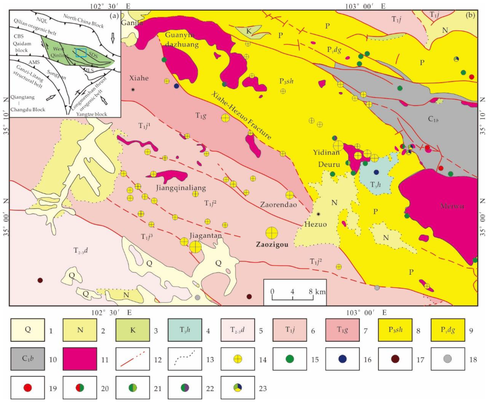
West Qinling is located at the western part of the Qinling orogenic belt, with the Qilian orogenic belt to the north, the Qaidam block to the west and the songpan block to the south (Figure 1a) [99,100,101,102].
The geotectonic position of the Xiahe–Hezuo area is located at the northwestern part of the West Qinling orogenic belt and at the western extension of the Qinling–Qilian–Kunlun central orogenic belt, whose complex geological structure creates a superior mineralization environment [103].
The Zaozigou gold deposit is located within the West Qinling fold belt and is a typical epithermal-type gold deposit in the Xiahe–Hezuo area (Figure 1a). The main controlling factors for mineral resources formation within the region are tectonic movement and magmatism [104], with the regional tectonics spreading in a NW direction with developing folds and fractures. Complex geological structure and magmatism are dominated by Yanshan period intermediate-acid intrusive rocks, which are widely distributed in the form of the batholith, stock, apophysis and veins [104] (Figure 1b).
Figure 1. (a) Geotectonic location of the study area. NQL: North Qinling tectonic belt; SDS: Shangdan suture zone; CBS: Caibei suture zone; AMS: A’nyemaqen suture zone. (b) Geological map of Xiahe–Hezuo area (modified from [104]). 1. Quaternary; 2. Neogene; 3. Cretaceous; 4. Upper Triassic Huari group; 5. Middle-Lower Triassic Daheba group; 6. Lower Triassic Jiangligou group; 7. Lower Triassic Guomugou group; 8. Upper Permian Shiguan group; 9. Lower Permian Daguanshan group; 10. Upper Carboniferous Badu group; 11. Intermediate-acid intrusive rocks; 12. Fracture; 13. Angular unconformity; 14. Gold deposit; 15. Copper deposit; 16. Lead deposit; 17. Antimony deposit; 18. Mercury deposit; 19. Iron deposit; 20. Iron-copper deposit; 21. Copper-molybdenum deposit; 22. Copper-tungsten deposit.
Minerals 12 01361 g001
The Triassic strata are the main stratigraphy for gold deposits. The genesis and spatial-temporal evolution of the intermediate-acidic dike is closely related to gold mineralization in the area, and during the mineralization process, the magmatic rocks not only provide the mineralized material, but also their internal environment is very suitable as an ore-bearing space, which can be regarded as a significant mineralization indicator for gold mineralization [105].
The spatial distribution of mineral deposits is directly controlled by the geotectonic position in the Xiahe–Hezuo area, which plays a major role in the formation of different types of gold deposits and is the boundary of the belt from a spatial perspective. The most important types of mineral-controlling structures are fractures and folds in this area [106,107]. The main orebodies of the Zaozigou deposit are produced in NE, NW and near-SN oriented fracture zones, with two apparent mineralization periods, and post-formation fractures have modified and destroyed the orebodies [108,109,110,111,112].
The Zaozigou gold deposit is a typical representative of gold deposits associated with intermediate-acid dike rocks in the south of the Xiahe–Hezuo fracture. It is located approximately 9 km southwest of Hezuo city, Gansu Province, with convenient access to the mine site (Figure 2a). The main ore-bearing position is between Gully 1 and Gully 4, with a total area of approximately 2.6 km2 (Figure 2b).
There are only Triassic and Quaternary strata exposed in the Zaozigou gold deposit (Figure 2b). The strata of the area are mainly the lower part of the Gulangdi group (T2g1) of the Middle Triassic formation, and the Quaternary (Qhalp) is developed in the intermountain valley. The lower part of the Gulangdi group (T2g1) is the main ore-bearing rock, which is a set of fine clastic rocks consisting of siliceous slate, clastic feldspathic fine sandstone with interbedded siltstone slate and argillaceous slate. The formation is composed of a large sedimentary cycle from bottom to top consisting of siltstone → argillaceous slate → calcareous slate [108,114].
The fractures are well developed and have a complex morphology, forming an intersecting trend, indicating that the area has experienced multiple phases of geological activity. Fractures strictly control the distribution of orebodies and vein rocks within the deposit. They can be classified into five groups of orientations, namely NW, N-S, NE, E-W and NNE [115,116]. Fracture structures are the structural surfaces of mineralization and these structural surfaces control the spreading characteristics of the orebodies [117].
Intermediate-acid dike, including fine crystalline diorite, diorite porphyrite, biotite dioritic porphyrite and quartz diorite porphyrite densely produced with a porphyritic structure, spreads in NNE direction, turning to a nearly N-S direction in the western part of the deposit and a few NW directions. Influenced by the regional multi-period deep fracture activity, the multi-period magmatism has overlapped on multi-phases mineralization within the deposit [118].
There are 147 gold orebodies that have been found in the Zaozigou gold deposit, of which 17 orebodies are main orebodies with gold reserves greater than 1 tonne and the total gold reserves amount to more than 100 tonnes [113]. According to the spatial distribution and combination of the mineralization, the Zaozigou deposit can be divided into eastern and western ore groups.
The eastern ore group is mainly located between Gully 1 and Gully 3 with the strike of NE orientation, containing Au1 controlled by F24, Au9 controlled by F21 and Au15 controlled by F25. These orebodies extend over 1000m long and 300m wide, with a NW direction tendency and steep dip near the ground surface, locally nearly upright. In the deep, these orebodies have been staggered by a gently dipping fracture, causing the tendency to change to a SE orientation (Figure 2b). In addition, orebodies M4 and M6 are laying underground, with the strike of NWW orientation, the tendency of SW orientation and a dip of 8°~26°. These orebodies cross the NE-striking orebodies obliquely, staggering them, and their own mineralization behavior occurs simultaneously [119].
The western ore group is mainly distributed between Gully 3 and Gully 4, spreading in a nearly N-S direction, with Au29~Au31 as the main orebodies. The orebodies extend over 1000 m long and are wider than 500 m, with a strike of 350°~10°, varying tendency and dips greater than 75°, locally subvertical. These orebodies extend, and the mineralization is weaker in the steeper parts and stronger in the shallower parts.

2.2. Datesets Description

Historical geological and geochemical data were completed, including geological reports, geological exploration maps, drills geochemical data, etc., from the Development Research Center of China Geological Survey and No. 3 Geological and Mineral Exploration team, Gansu Provincial Bureau of Geology and Mineral Exploration and Development; the coordinate system used in the mine-scale is Gaussian Kruger projection coordinates.
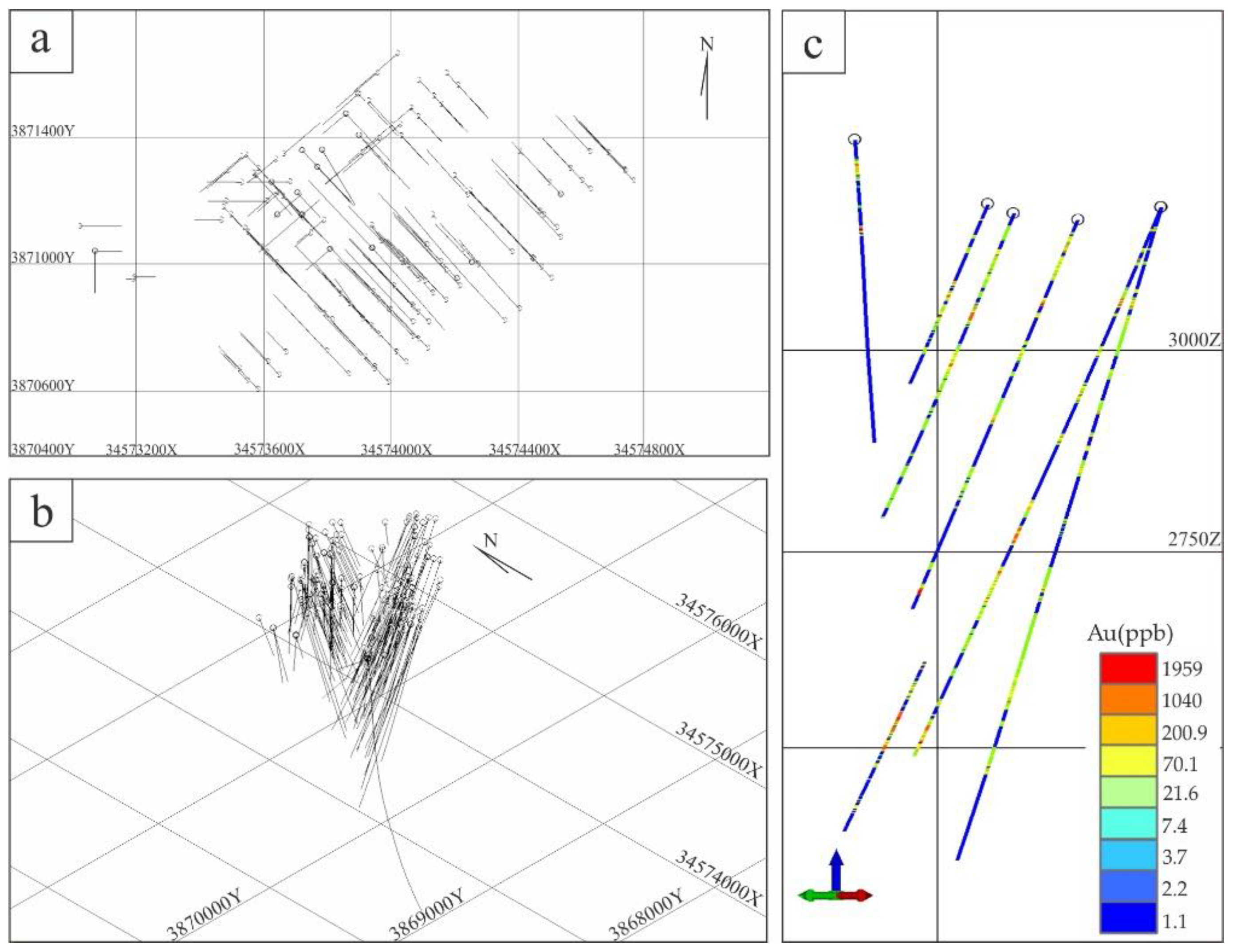
This study collects data from 72 drillings in the Zaozigou gold deposit and establishes a drilling location database, an assay database, an inclinometry database and a lithology database. The 3D model of drillings is constructed based on the drill hole data database (Figure 3).
The primary geochemical halo data from the drillings are collected from the “Zaozigou gold successive resources exploration project in Hezuo city, Gansu Province”, with a total of 72 drillings and 5028 samples with 12 elements of Ag, As, Au, Cu, Hg, Pb, Zn, Sb, W, Bi, Co and Mo (the element detection methods can be seen in the literature [113]). The sampling method was the continuous picking method with sample intervals generally within 10m. Some orebodies or strongly altered areas were sampled at decreased intervals.

3. Methodology

3.1. Concentration-Volume (C-V) Model

Geochemical anomalies are a concept relative to geochemical background, and the multifractal approach provides an effective tool to separate anomalies from the background. For hydrothermal mineralization processes, multi-phase mineralization is common, which will result in multi-phase superposed element spatial distribution [38,120,121]. The C-V model can process the nonlinear primary geochemical halo data with the following equation:
V ( ρ < v ) k v D 1 V ρ v k v D 2
where V ( ρ < v ) and V ρ v are the volumes of the element content less than v and greater than v ; D 1 and D 2 are the fractal dimension values, also called the singularity index; k is a constant coefficient, which can be calculated by the least square method; v is the threshold value of element contents, and several element content intervals are divided by v. The curves V ( ρ < v ) and V ρ v of the volumes corresponding to different v follow a power-law relationship. Taking the natural logarithm of both sides of the equation, the lg-lg plots have a linear relationship in different v intervals. The fractal dimensions in different v intervals can be calculated by the least square method. The geochemical anomalies and backgrounds can be extracted by different fractal dimensions [39].
In practice, the C-V model is used on the primary geochemical halo data volume model for anomaly identification, where the threshold of fractal dimensions may indicate the boundary between different mineralization.

3.2. Compositional Data Analysis

Geochemical data, as typical of compositional data, should be properly transformed before data analysis [122,123,124,125] to eliminate the effects of “closure effects”. The “opened (transformed)” data can often be analyzed by classical statistical methods to obtain performance improvements [36,53,61,122].

3.2.1. Central Log-Ratio Transformation (clr)

The calculation of this method is: (i) calculate the geometric mean of all compositional subvectors; (ii) divide each subvector by the geometric mean separately; (iii) take the natural logarithm. Its calculation formula is shown as follows.
clr x = l n x 1 i = 1 D x i D , l n x 2 i = 1 D x i D , , l n x D i = 1 D x i D

3.2.2. Sequential Binary Partition (SBP)

The common isometric log-ratio transformation (ilr) is difficult to interpret. Egozcue [50] proposed the sequential binary partition (SBP) technique based on the ilr transformation, which can provide geochemical interpretation reasonably [66,123,124].
The sequential binary partition technique performs non-overlapping dichotomous classification continuously by the relative information between variables. In practice, positive (+) and negative (−) signs are used to represent two different classifications of compositional variables, and ‘0’ is used to represent the unconcerned variables in one time. By performing continuous non-overlapping dichotomy in a simplex space, a basis vector is formed and then transformed. The results, called compositional balance, can be geologically interpreted according to dichotomy clusters. Especially, the technique provides an important tool to identify element associations [66,123,124,126].
The relevant formula is [50]:
B i = r i s i r i + s i l n ( + x j ) 1 r ( x k ) 1 s i = 1 , 2 , , D 1 ;   j = 1 , 2 , , r ;   k = 1 , 2 , , s
where B i denotes the new compositional vector defined by the standard orthogonal basis, + x j is the product of the variables labeled (+) involved in the ith binary partition and x k is the product of the variables labeled (−) involved in the ith binary partition.

3.2.3. Geochemical Compositional Data Analysis Framework Based on CoDA

The log-ratio transformation of geochemical data can solve the problem of the “closure effect” caused by the lack of scale consistency in the covariance matrix of the compositional data. The clr-biplot and compositional balance methods developed based on the clr and SBP have their advantages in the geochemical associations’ extraction, especially in inferring lithology, faults, alteration and mineralization, and the corresponding frameworks have been well applied [65,66,124].
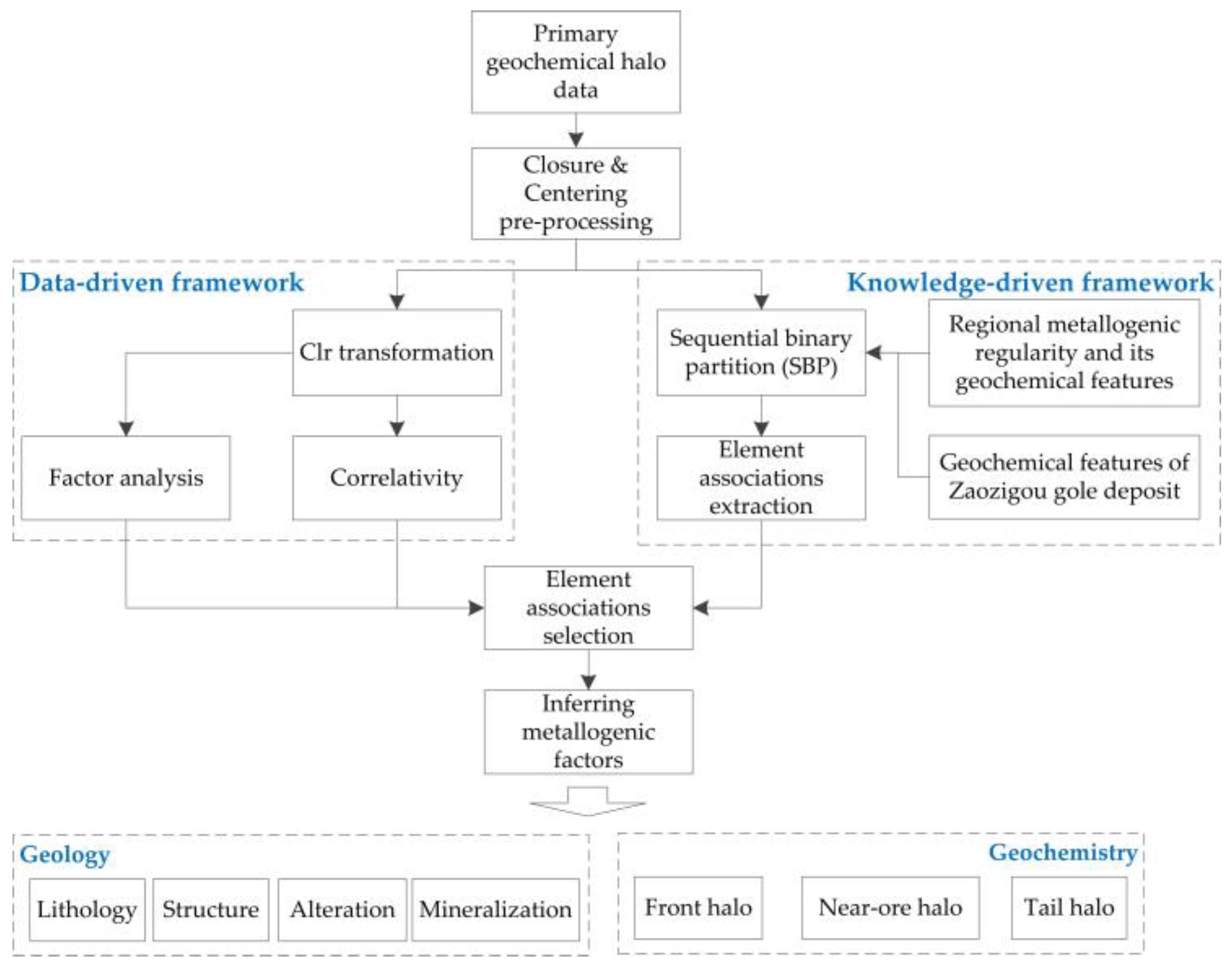
This study uses a data-driven and knowledge-driven framework of compositional data analysis to identify the geochemical associations of the primary halo. The data-driven framework infers the data characteristics by measuring elemental statistical correlations to gain the element associations, while the knowledge-driven framework is based on geological and geochemical understanding to design the element associations (Figure 4).
In Figure 4, the closure and centering are necessary preprocess steps, which can can be seen in the literature [51]. The data-driven framework in this study used clr transformation to “open” geochemical data, and the factor analysis and correlativity methods are used to explore the relationship among elements and extract element associations. Meanwhile, the knowledge-driven framework designs the element associations through deep research of the geological features, such as the element concentrations in different rocks, the primary geochemical halo associations, and so on. Then, the SBP is performed to quantitatively extract the value of corresponding geochemical associations. Eventually, the results of the CoDA can be employed to infer metallogenic information in an unknown area.

3.3. Machine Learning-Based Quantitative Mineral Prediction Methods

Machine learning algorithms could highlight hidden details in datasets without explicit search and have the ability to identify complex spatial patterns [127]. Given this, scholars have attempted to use machine learning algorithms to extract mineralization information by integrating multi-source geosciences data for identifying mineralization-related anomalies and their variation that cannot be detected by traditional methods [128,129,130,131,132,133,134,135]. Machine learning algorithms can be roughly categorized as supervised learning algorithms and unsupervised algorithms. For better validating the suitability of 3D MPM, this study discusses the application of the supervised algorithm MaxEnt model and unsupervised algorithm GMM.

3.3.1. MaxEnt Model

The principle of MaxEnt is a criterion of probabilistic model learning for making predictions based on incomplete information. The main idea is that, when predicting the probability distribution of a random event, all known constraints need to be satisfied without subjective assumptions so that the probability distribution is most uniform, the prediction risk is minimal and the entropy value of the probability distribution is maximum [136].
Let T = x 1 , y 1 , x 2 , y 2 , ( x n , y n be the training dataset and f i x , y , i = 1 , 2 , , n be the eigenfunction, and the learning process of the MaxEnt model is equivalent to the constrained optimization problem:
m a x P C H P = x , y P ˜ x P y x l n ( P y x ) s . t . E P f i = E P ˜ f i i = 1 , 2 , , n y P y x = 1
where E P ˜ f i = x , y P ˜ x , y f i x , y is the expected value of n eigenfunction f i x , y related to the empirical distribution P ˜ x , y ; E P ˜ f i = x , y P ˜ x P y x f i x , y is the expected value of n eigenfunctions f i x , y related to the P Y X with the empirical distribution P ˜ X .
Following the custom of optimization problems, the problem of finding the maximum value is rewritten as the equivalent problem of finding the minimum value:
m i n P C H P = x , y P ˜ x P y x l n ( P y x ) s . t . E P f i E P ˜ f i = 0 i = 1 , 2 , , n y P y x = 1
The solution resulting from solving the constrained optimization problem is the solution learned by the MaxEnt model. However, the empirical distribution expectation is usually not equal to the true expectation but will be approximate to the true expectation. If the solution is solved strictly according to the above constraints, it is easy to cause overfitting of the training data during the learning process. Therefore, the constraints can be appropriately relaxed in practice, such as replacing the above equation with E P f i E P ˜ f i β i , β i is the modulation multiplier, which is a constant.

3.3.2. Gaussian Mixture Model (GMM)

GMM is a quantified model which generated through Gaussian probability density function fitting. This model decomposes objective distribution into several Gaussian probability density functions. By using enough Gaussian functions and tuning the parameters, the model can generate a very complex probability density to approximate to almost any continuous probability. Theoretically, any objective distribution can be fitted by a combination of multiple Gaussian density functions, and the higher the number of probability density sub-functions, the more closely it approximates to the actual data distribution. GMM has the advantages of good flexibility, is not limited by the sample size and can accurately describe the data structure.
When the dataset X = X 1 , X 2 , , X T of the training data can be divided into k classes and each class obeys Gaussian distribution, the k order probability distribution of the GMM is
P X θ = i = 1 k w i P X θ i
P X θ i = 1 2 π D 2 i 1 2 e x p 1 2 ( X μ i ) T i 1 X μ i
i = 1 k w i = 1 , w i > 0
where P X θ i is the probability density of the i th Gaussian model, w i is the weight of the i th model in the whole GMM, μ i is the mean vector and i is the covariance matrix. After the parameter initialization, the Expectation-Maximization (EM) algorithm based on the maximum likelihood estimation is often chosen for the parameter estimation of the GMM [137].
In the geological point of view, the GMM is an unsupervised machine learning algorithm; it divides the data into two categories (mineralization and non-mineralization) and then makes category judgments on samples by learning information about unlabeled samples.
As for the dataset D = x 1 , x 2 , , x m , which contains k Gaussian mixture components, the algorithm steps are as follows.
  • Initializing the k multivariate Gaussian distributions and their weights.
  • Estimating the posterior probability of each sample generated by each component according to Bayes’ theorem.
  • Updating the mean vector, covariance matrix and the weights according to the step 2.
  • Repeating steps 2–3 until the increase in the likelihood function has been less than the convergence threshold, or the maximum number of iterations is reached.
  • For each sample point, calculating its posterior probability of belonging to each cluster according to Bayes’ theorem and classifying the sample into the cluster with the largest posterior probability.

4. Results

4.1. Three-Dimensional Primary Geochemical Halo Anomaly Data Volume Modeling Based on the C-V Model

This section adopts the multifractal C-V model to analyze the spatial anomalous structure of elements and provides single-element anomaly signatures for the subsequent deep prediction.
Taking the ore-forming element Au as an example:
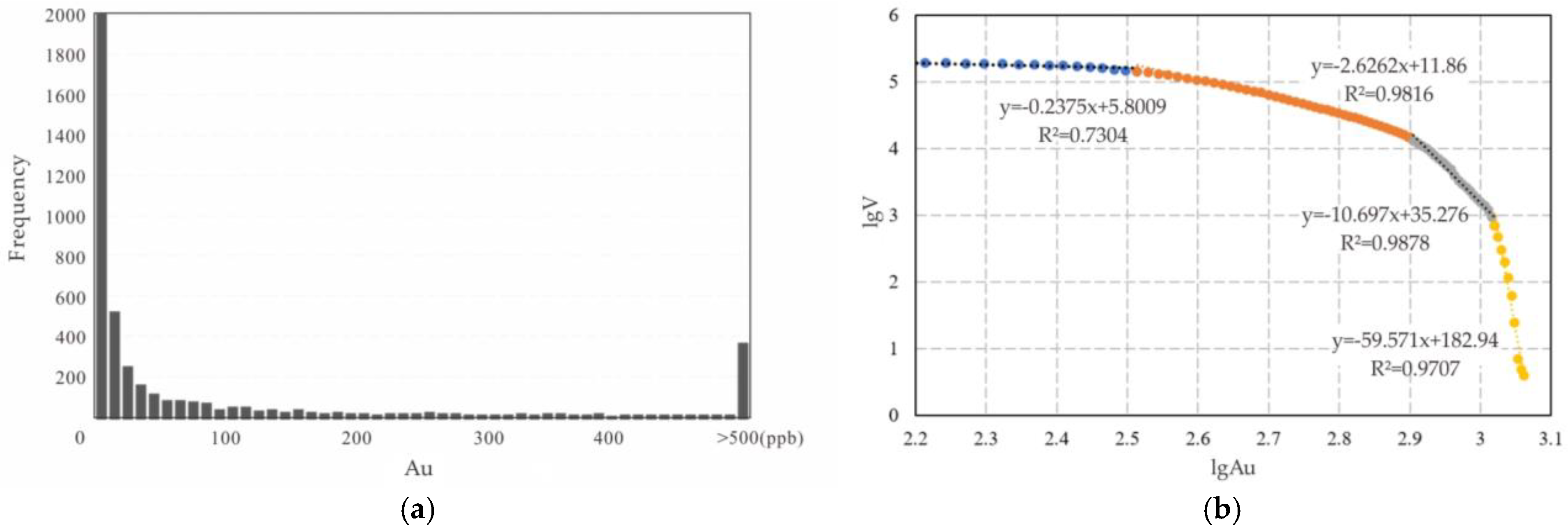
Using the ordinary kriging interpolation method [138,139,140], with the experimental variogram fitted to build a 3D data volume model of Au (Figure 5), the Au content value observably does not obey the normal distribution (Figure 6a). Therefore, the multifractal C-V model was carried out to identify Au anomalies.
Through counting the variation of volume with Au content, the lgAu-lgV scatter diagram was generated and lg-lg lines were fitted by the least square method (Figure 3b). Meanwhile, the fractal dimension can be obtained as follows:
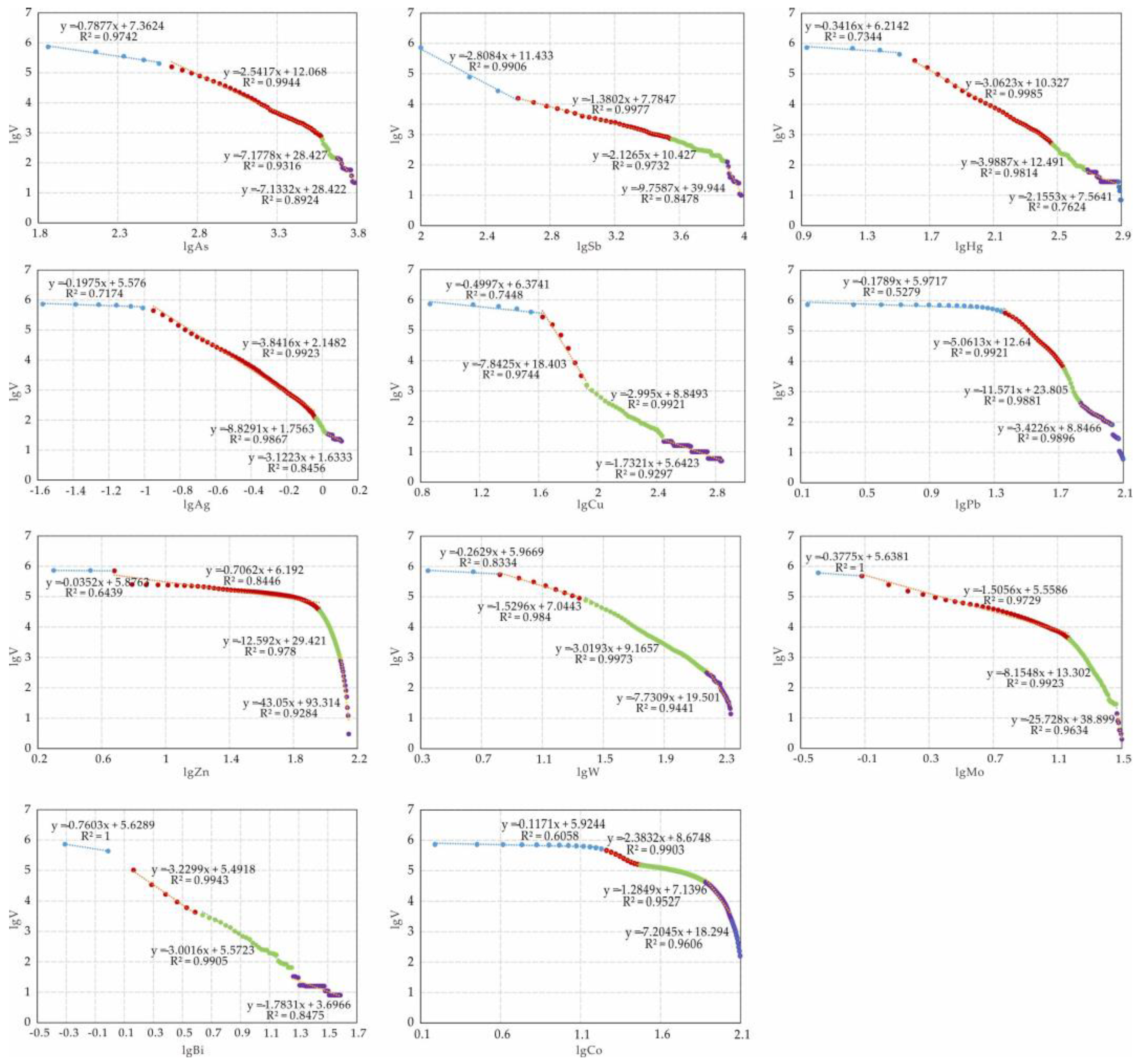
The slopes of the lines correspond to fractal dimensions, and the inflection points are threshold values of geochemical abnormal intensity as shown in Table 1 and Figure 6b.
The orebody is compared with the outside anomalies, central anomaly and internal anomaly area by superposition, as shown in Figure 7b,c, and the three show a good spatial correlation with the orebody.
The middle and inner anomalies are mainly distributed inside and around the orebody, which accurately reflects the spatial spreading of the orebody and its trend.
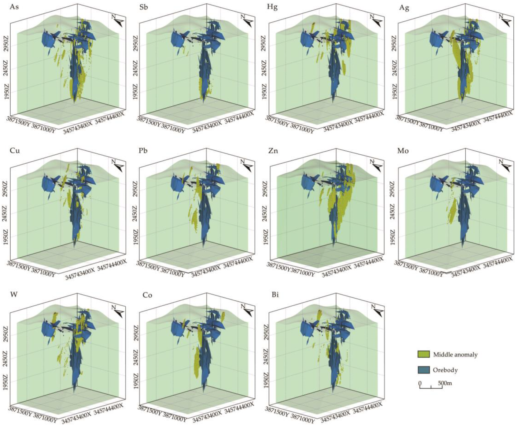
On this basis, this study analyzed and visualized the 3D anomalous structures of the remaining 11 elements using the above model (Figure 8; Table 2).
Figure 9 shows that the middle anomalies of As and Sb are mainly distributed near the elevation of 1700~1900 m. The middle anomalies of Ag, Cu, Pb and Zn have close relationship to the orebody. W, Mo, Co and Bi have two concentrations, the first one is located near the surface and the second one is distributed near the elevation of 2500 m. The Zaozigou gold deposit has multi-phase mineralization, forming a complicated spatial distribution of elements, while the C-V model can better identify the anomaly for recognizing the pattern of the primary geochemical halo in the Zaozigou gold deposit.

4.2. Data-Driven CoDA and Its Based Element Association Extraction

4.2.1. Correlation Analysis

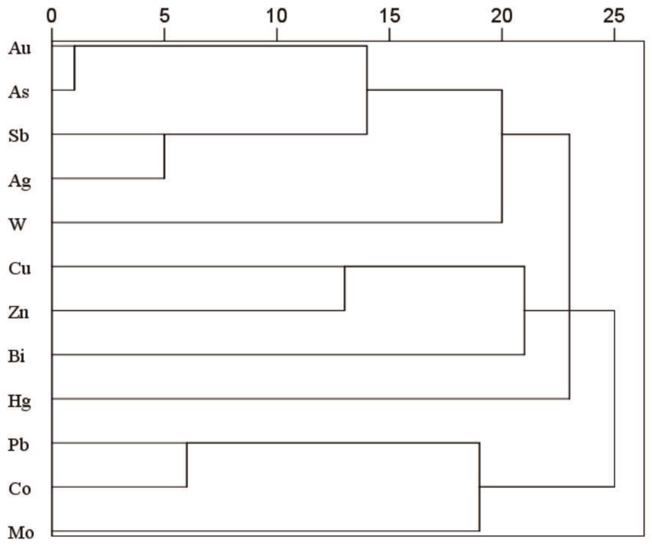
The primary halos were processed by cluster analysis (Figure 10). The elements can be roughly divided into two groups: Au, As, Sb, Ag, W, Hg and Cu, Zn, Bi, Pb, Co, Mo. Among them, the elements most closely associated with Au are As, Sb and Ag; the Au, As, Sb and Cl are moderate volatile elements [141] often associated in gold mineralization like Hg (indicator of volcanism). Ag is often associated to gold as electrum. Hg should be the front halo indicating element of the gold orebody; the correlation coefficient between Au and As reaches 0.8, and most of the As exists within arsenopyrite, which is an important gold-bearing mineral. Therefore, this Au-As-Sb should be the element association of mineralization reflecting a middle- and low-temperature metallogenic environment.

4.2.2. Element Associations Identification Based on clr-Biplot

Geochemical data are typically compositional data, and if traditional multivariate statistical methods (e.g., principal component analysis, factor analysis, etc.) are applied directly to the raw geochemical data, it may lead to erroneous results. Therefore, the raw data should be properly transformed before data analysis is performed.
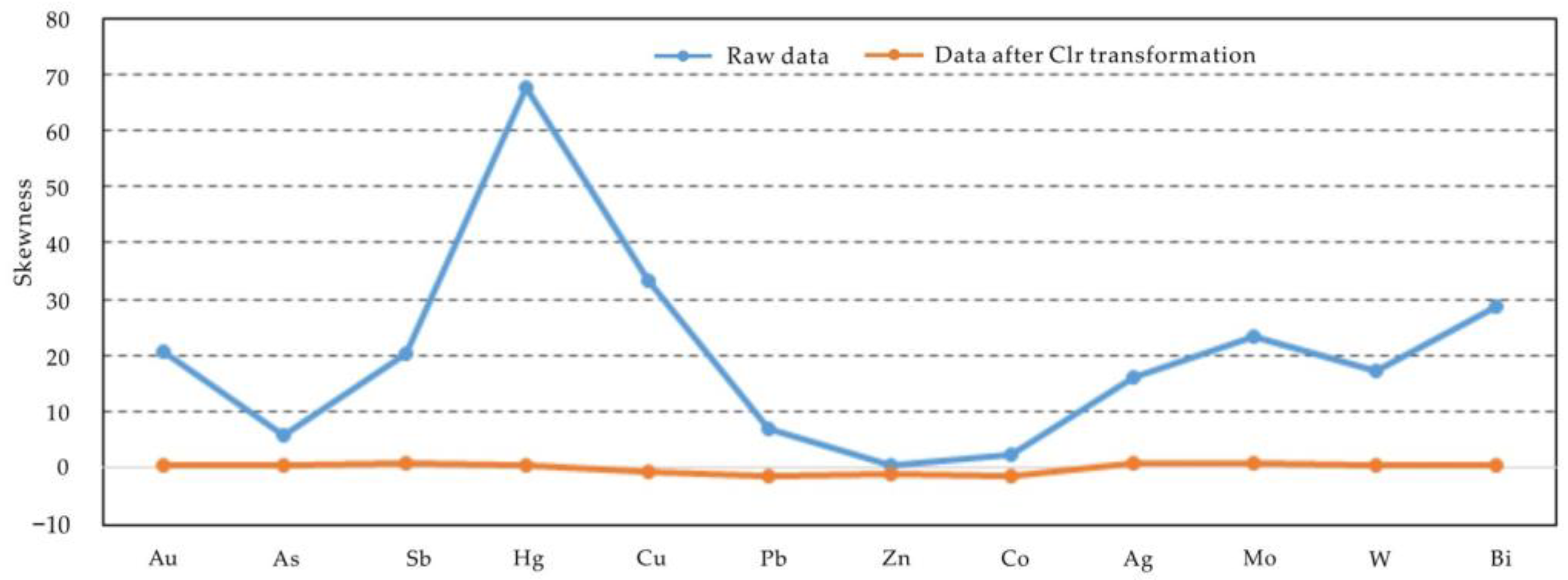
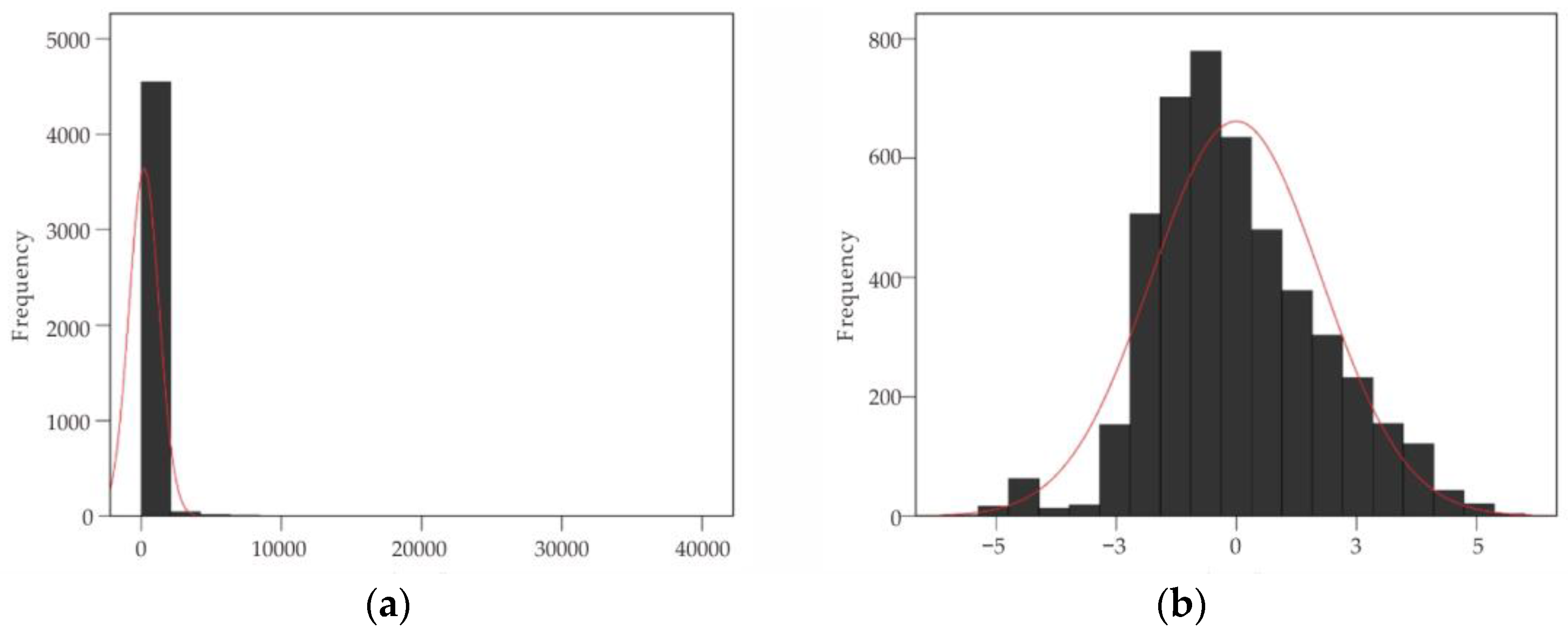
Data from 12 geochemical elements were clr-transformed, and the skewness values of the clr-transformed data were statistically obtained (Figure 11). Compared with the raw data, clr-transformed data has the lower skewness value around zero, indicating that the data distribution after clr transformation tends to be more normal in character (Figure 11 and Figure 12).
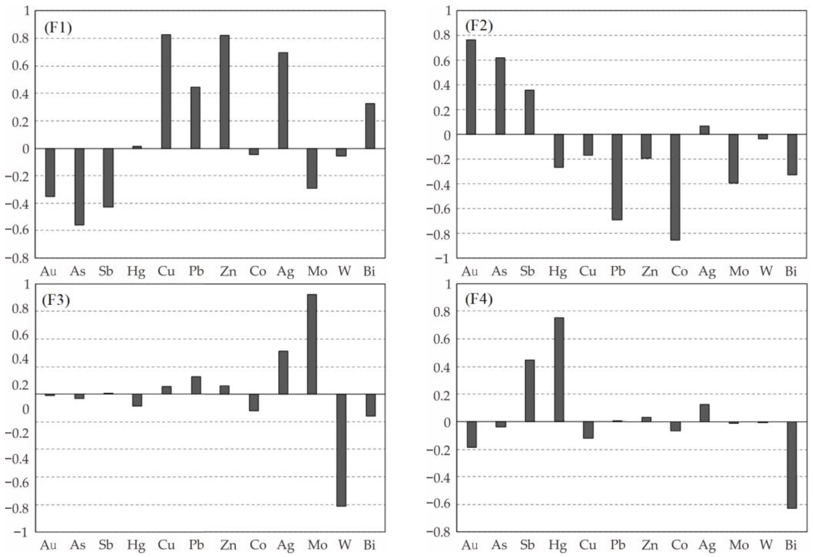
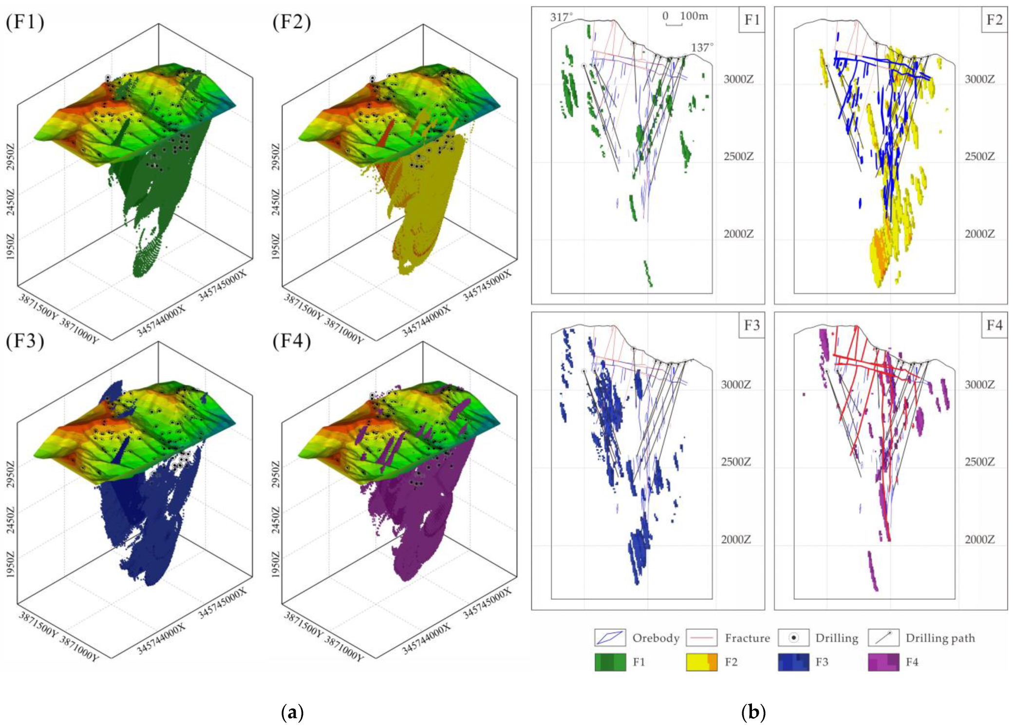
Factor analysis (FA) is used to extract element associations. Four factors are extracted as element associations to indicate different geological and geochemical meanings. From the view of the loadings of FA, factor F1 (34.95%, five variables) represents Cu, Pb, Zn, Ag and Bi, which are a group of medium-temperature elements; factor F2 (12.83%, three variables) is the element association of Au, As and Sb, representing the Au-polymetallic sulfide phase, which is the most dominant phase of gold mineralization; factor F3 (11.13%, one variable) indicates Mo, which is a high-temperature element and may be related to magmatism; factor F4 (9.26%, two variables) is Sb and Hg association, where Sb mainly exists within the form of stibnite within the quartz-stibnite veins and Hg is closely related to fractures (Figure 13). The distribution of each factor in the three-dimensional space is shown in Figure 14a.
To analyze and show the geological meaning of each factor more clearly, the 85# profile was selected for analysis by profile cutting (Figure 14). It can be intuitively understood that the F2 factor is closely related to mineralization, and its spatial distribution is well matched with the known orebodies in the exploration profile. The F4 factor is closely related to ore-bearing fractures, so that the Sb-Hg element association could be used as evidence of deep fracture extension.

4.3. Knowledge-Driven CoDA and Its Based Element Association Extraction

From the anomaly data volume model based on the C-V method in this paper, it is clear to recognize the distribution of each element in a three-dimensional space.
1.
In the mid-shallow part and the deeper part of elevation at 2500 m, As, Sb and Hg are concentrated as the front halo of the orebodies. The anomalies of Au, Ag, Cu, Pb and Zn linked to sulphurs (pyrite, arsenopyrite, galena and covelline) and are superposed with the orebodies and can be regarded as the near-ore halo elements. At the shallow position of 2500 m, the anomaly locations of W, Mo and Bi linked to magmatism are at the tail of the orebodies, which can be regarded as the tail halo element association.
2.
In terms of Au, its anomalies are controlled by fractures observably, and observable fractures certainly cross-cut orebodies. Especially, the abnormal intensity is larger along the depth indicating the deep mineralization.
Based on the analysis above, the knowledge of the element associations of the front halo, near-ore halo and tail halo can be summarized. Moreover, corresponding element associations are quantitatively extracted as compositional balances by the knowledge-driven CoDA framework (Figure 4), that is, the front halo association is B1 (As-Sb-Hg vs Au-Ag-Cu-Pb-Zn-W-Bi-Co-Mo), the near-ore halo association is B2 (Au-Ag-Cu-Pb-Zn vs As-Sb-Hg-W-Bi-Co-Mo), and the tail halo association is B3 (W-Bi-Co-Mo vs As-Sb-Hg-Au-Ag-Cu-Pb-Zn) (Figure 15).

4.4. Geological and Geochemical Quantitative Prediction Model at Depth of Zaozigou Gold Deposit

The mineral resources prediction model is usually summarized as text, diagrams, and tables by integrating comprehensive metallogenic information, such as orebodies, ore deposits, ore fields and even metallogenic zones. Establishing a mineral resources prediction model is an effective way to discover potential deposits and has significantly important meaning for guiding mineral exploration [142].
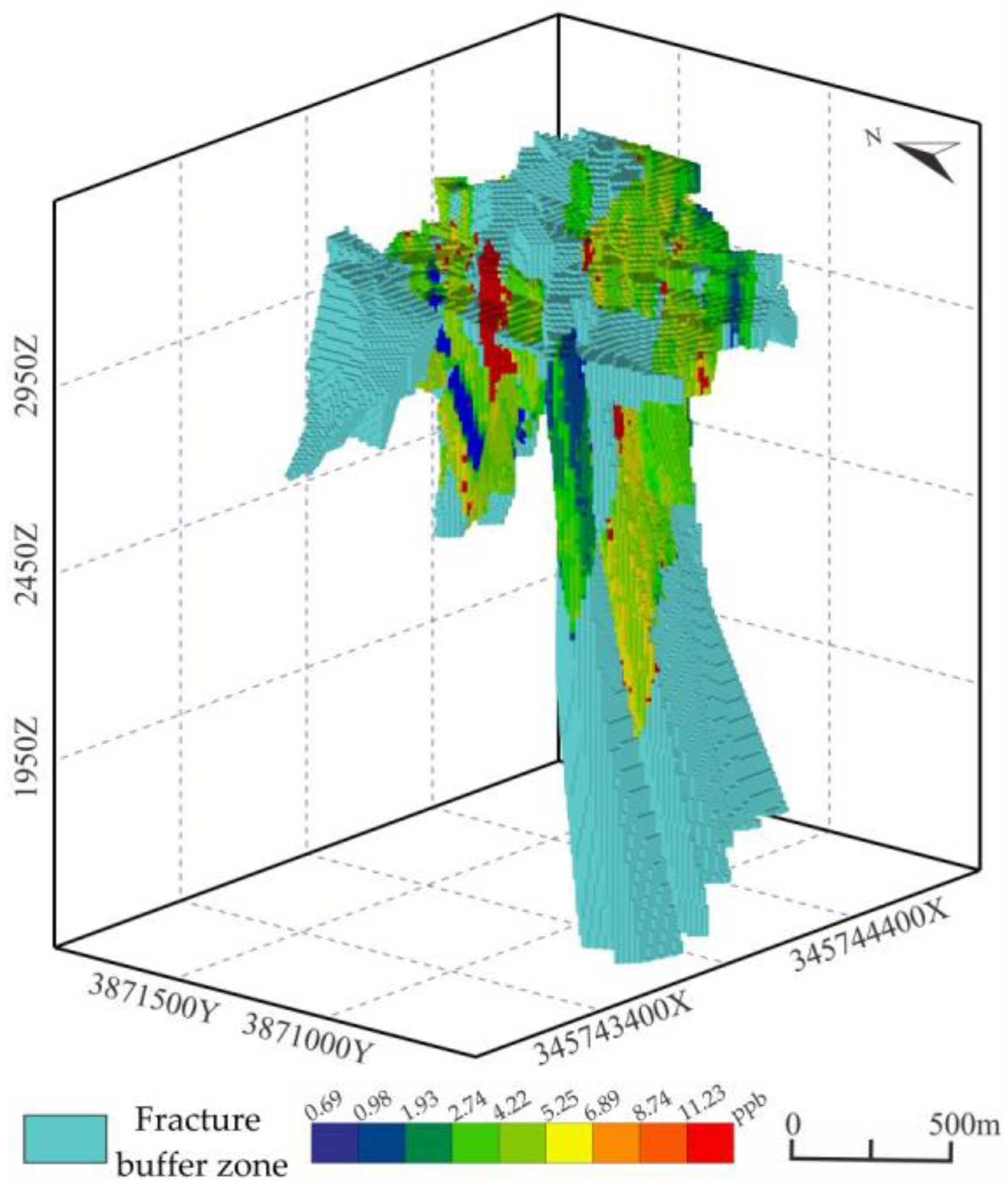
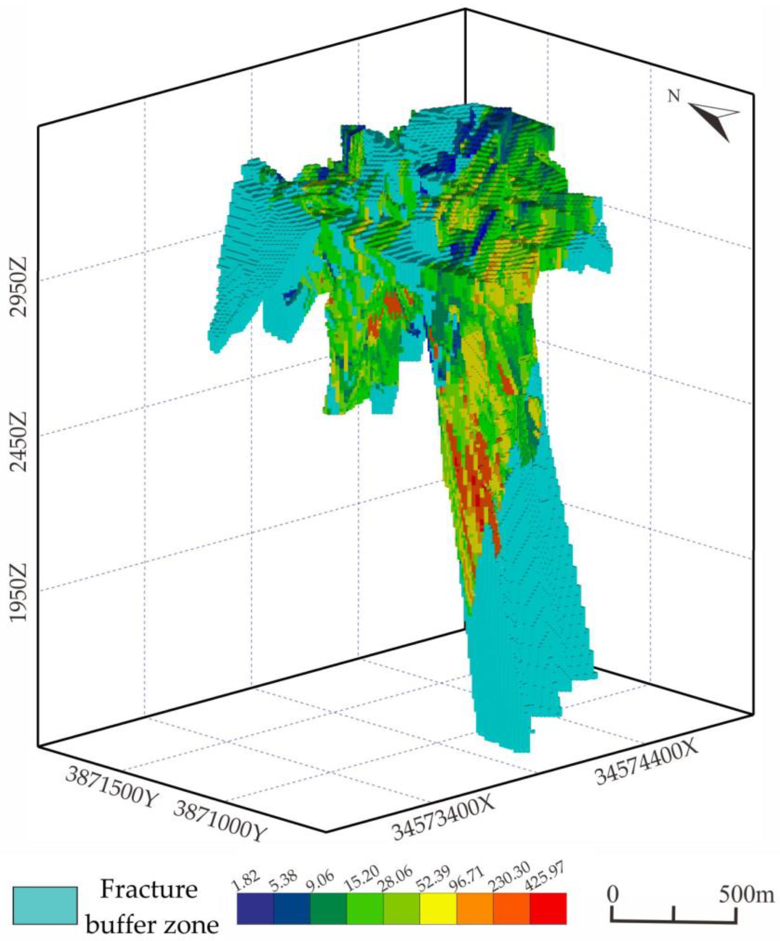
Orebodies are strictly controlled by fractures in the Zaozigou gold deposit. The 30 m buffer zone of the fractures can effectively reflect the influence range of the fracture, which can be used as a mineral prediction indicator. Factor F4 is an element association of Sb-Hg, which has close relationship with fractures, and can be used as a favorable indicator for inferring deep fractures [143,144,145,146] (Figure 14a).
Geochemical element distribution, association and zonation are favorable indicators for mineral resources prediction. The geochemical anomalies are extracted by the multiple fractal C-V model in Section 4.1, among which the middle anomaly of Au can well reflect the spatial distribution of orebodies (Figure 7b) and should be used as an important quantitative indicator. Near-ore halo element association B2 is extracted by the knowledge-driven CoDA and also can express the location of orebodies well; it should be another mineral prediction indicator (Figure 15). The ratio of front halo to tail halo is an important geochemical parameter for predicting orebodies, and B1/B3 is regarded as a prediction indicator accordingly [143] (Figure 16).
In summary, the geological and geochemical quantitative prediction model at the depth of the Zaozigou gold deposit is constructed as in Table 3.

4.5. Three-Dimensional MPM Based on Machine Learning

To address the scientific problem of quantitative mineralization prediction at large depths, the previous section quantitatively extracted the deep geochemical mineralization signatures and constructed a geological and geochemical quantitative mineral resource prediction model at depth. In this section, the MaxEnt model and GMM are applied to carry out the 3D MPM to quantitatively predict deep mineral resources, and the uncertainty evaluation of the two models is performed for improving the accuracy of mineralization prediction.

4.5.1. Training Sample Construction

The MaxEnt model is a supervised machine learning algorithm, which requires learning an optimal model from a given training dataset and using this model to output the corresponding result for classification.
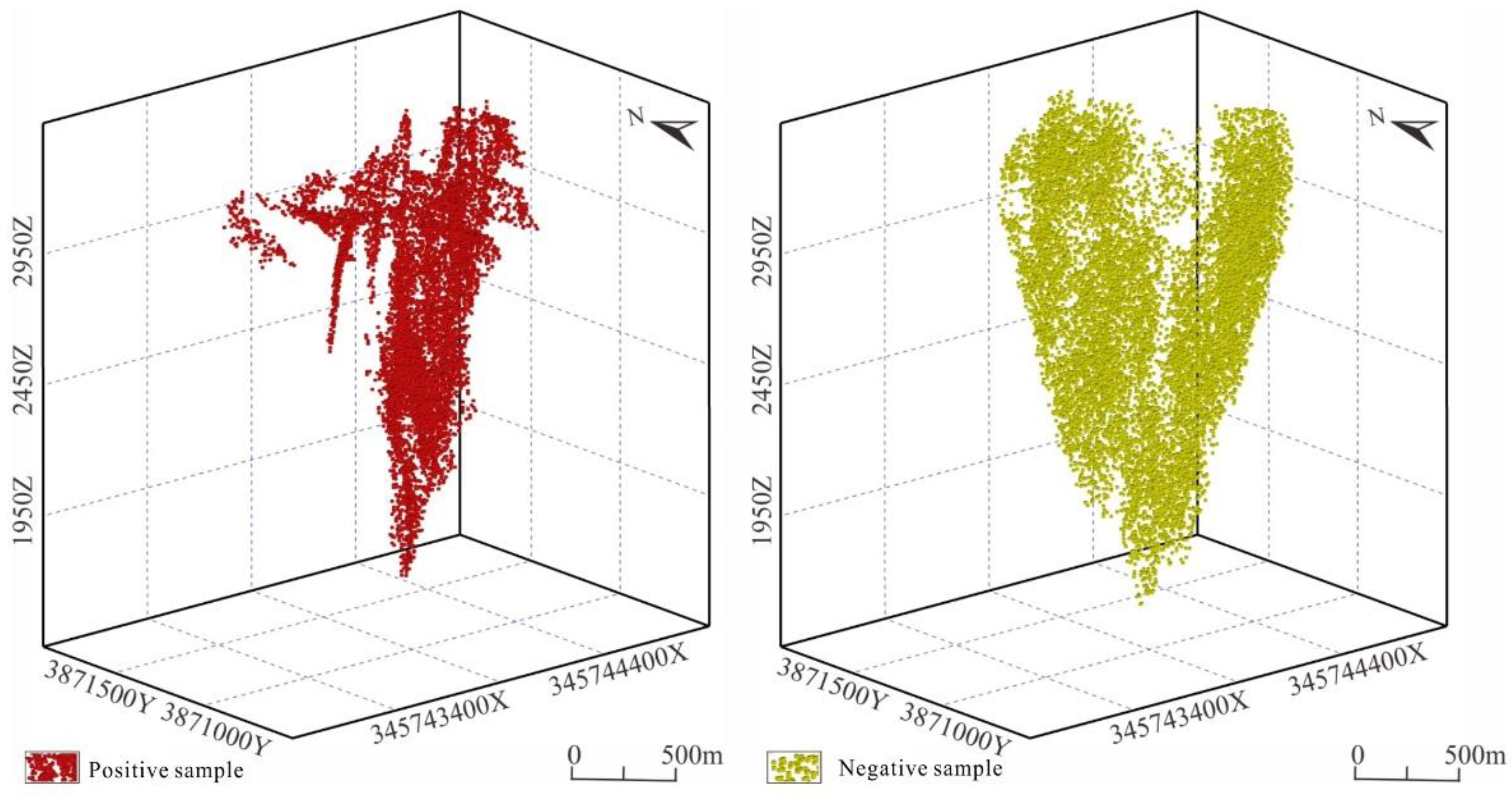
For mineralization prediction, the target variable of supervised learning (i.e., the label of training samples) is either mineralized or nonmineralized (denoted by 1 and 0, respectively). A total of 39,306 positive samples were extracted from known orebodies and 49,686 negative samples were extracted from the nonmineralized position confirmed by drillings, and these were used as the training dataset. In contrast to mineralization, which generates in a concentrated way in a limited space, the non-mineralization is a widespread phenomenon, and negative samples are selected to be distributed as randomly and uniformly as possible in the wall rock without mineralization and alteration throughout the study area [33] (Figure 17).

4.5.2. Three-Dimensional MPM and Uncertainty Evaluation of MaxEnt Model

The MaxEnt method originated from statistical mechanics and was developed by Phillips et al. using JAVA. This study uses version 3.4.1 of MaxEnt software (https://biodiversityinformatics.amnh.org/open_source/maxent/, (accessed on 15 June 2022)) to carry out the 3D MPM.
The MaxEnt method estimates the probability of the target variable with the maximum entropy value and is controlled by a set of constraints representing incomplete information about the target distribution. In mineralization prediction, the best interpretation of unknown occurrences by the model is to maximize the entropy value of the probability distribution for estimating the location of orebodies, and many scholars have achieved better results in this regard [65,76,147]
When modeling with MaxEnt software, if the model parameters are not set properly, it may lead to overfitting or redundancy [148]. The overfitting can be controlled by the modulation multiplier β [149], and the best performance of the model is obtained by setting the β value 2~4 [148,150]. Therefore, the study tested different values to find the best β value of 2 for the model to reduce the influence of model overfitting.
Five prediction indicators are integrated into the MaxEnt model as input parameters, and data were randomly selected from the dataset during simulation, with 75% of the dataset as the training data and 25% as the test data. To reduce the randomness of the simulation results, the model is repeated 50 times with a maximum convergence threshold of 0.00001. A maximum background points value of 10,000 is selected, and a logical value format output is chosen for a more favorable interpretation of the results.
The final prediction result of the MaxEnt model is evaluated using the average value of 50 iterations of the simulation, with the contribution rate of each mineral indicator shown in Table 4.
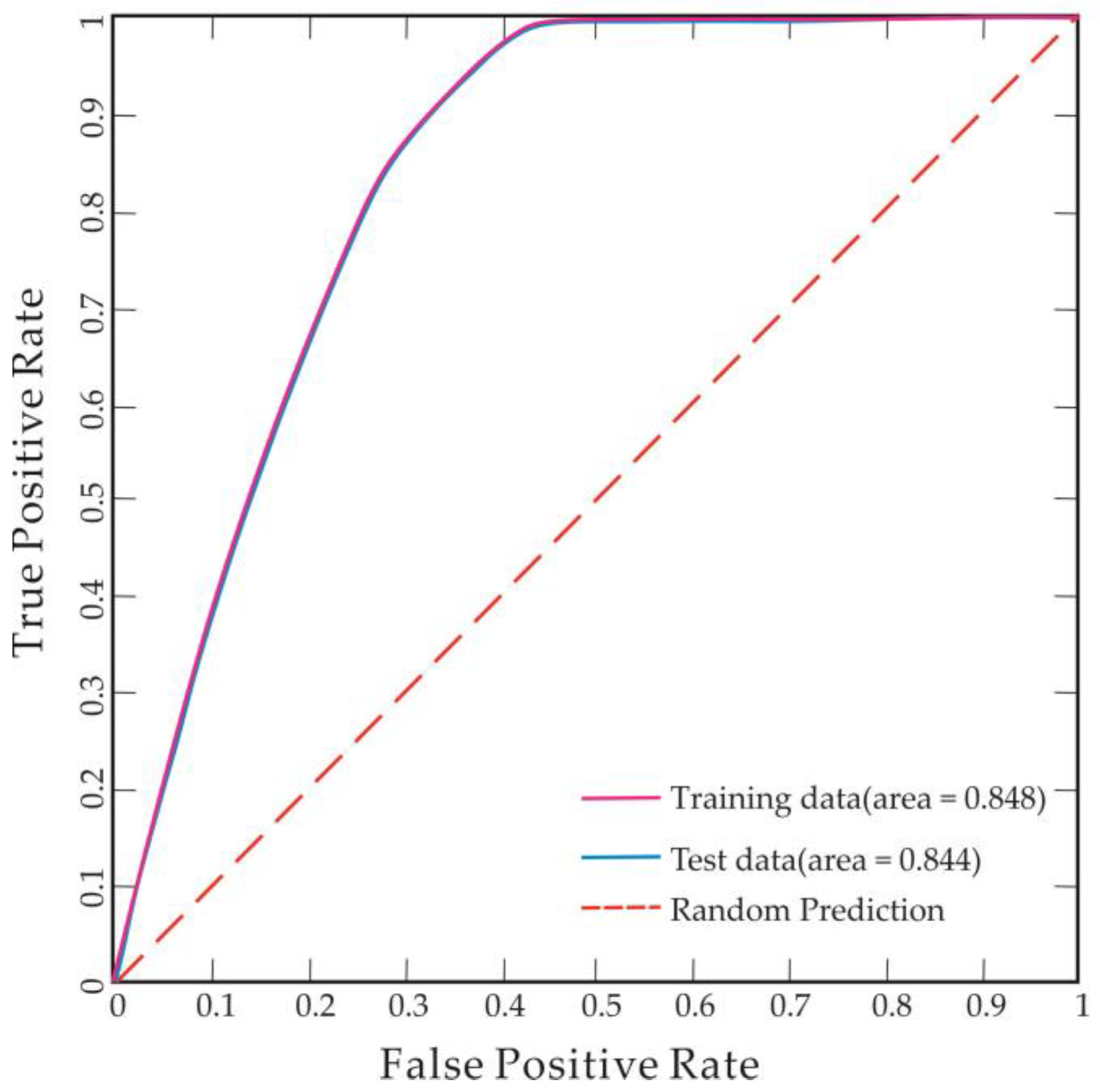
The AUC value of the test dataset is 0.844 and the AUC value of the training dataset is 0.848, so the MaxEnt model has high accuracy in mineral resources prediction at depth (Figure 18).
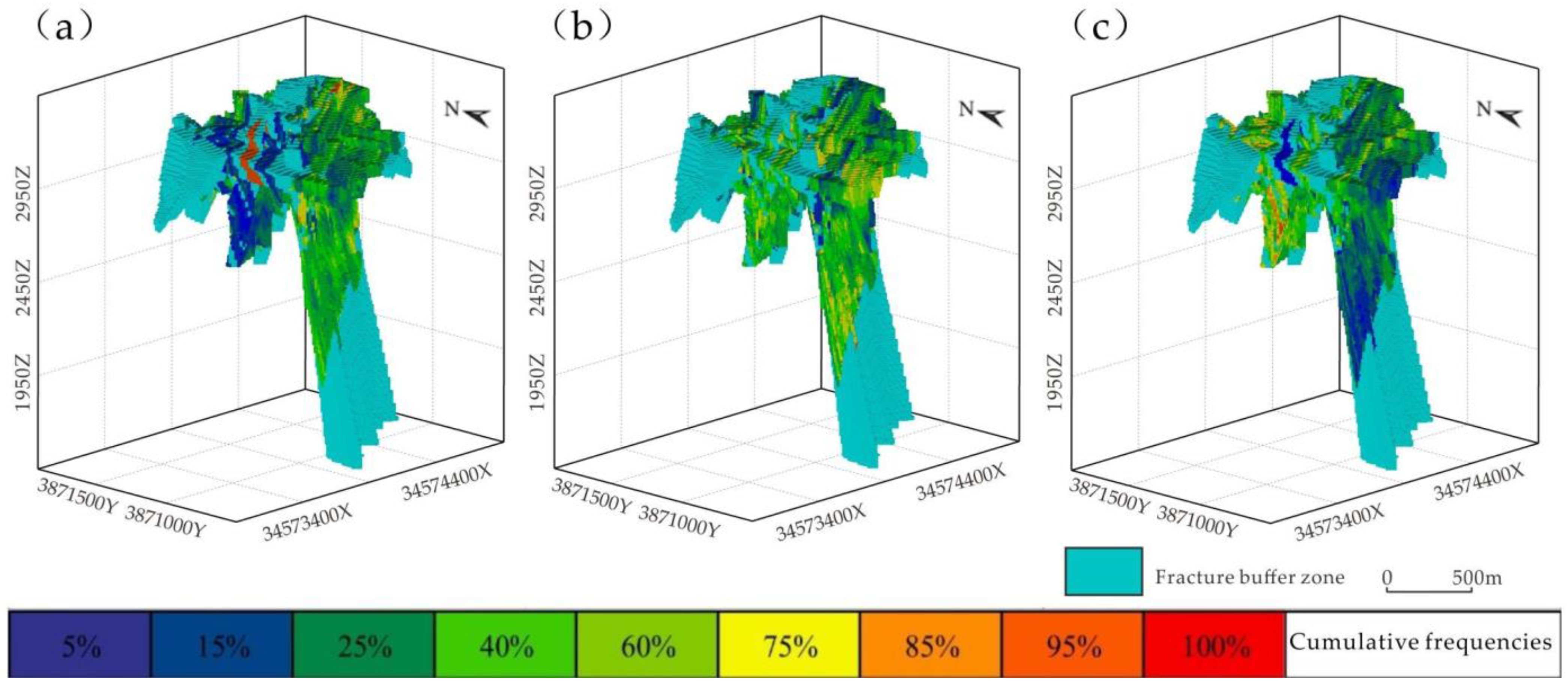
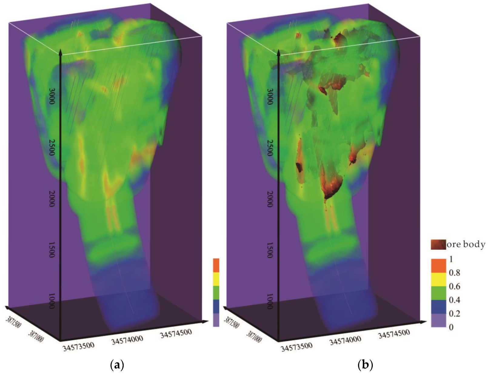
The output logical probability of the MaxEnt model is in the range of 0.000804~0.927941, which is mapped to 0 and 1, and then the 3D MPM is formed (Figure 19).
Although the mineral prospectivity map shows a good relationship between high probabilities and known gold orebodies (Figure 19), it is difficult to determine a certain logistic probabilities value as the prediction threshold value.
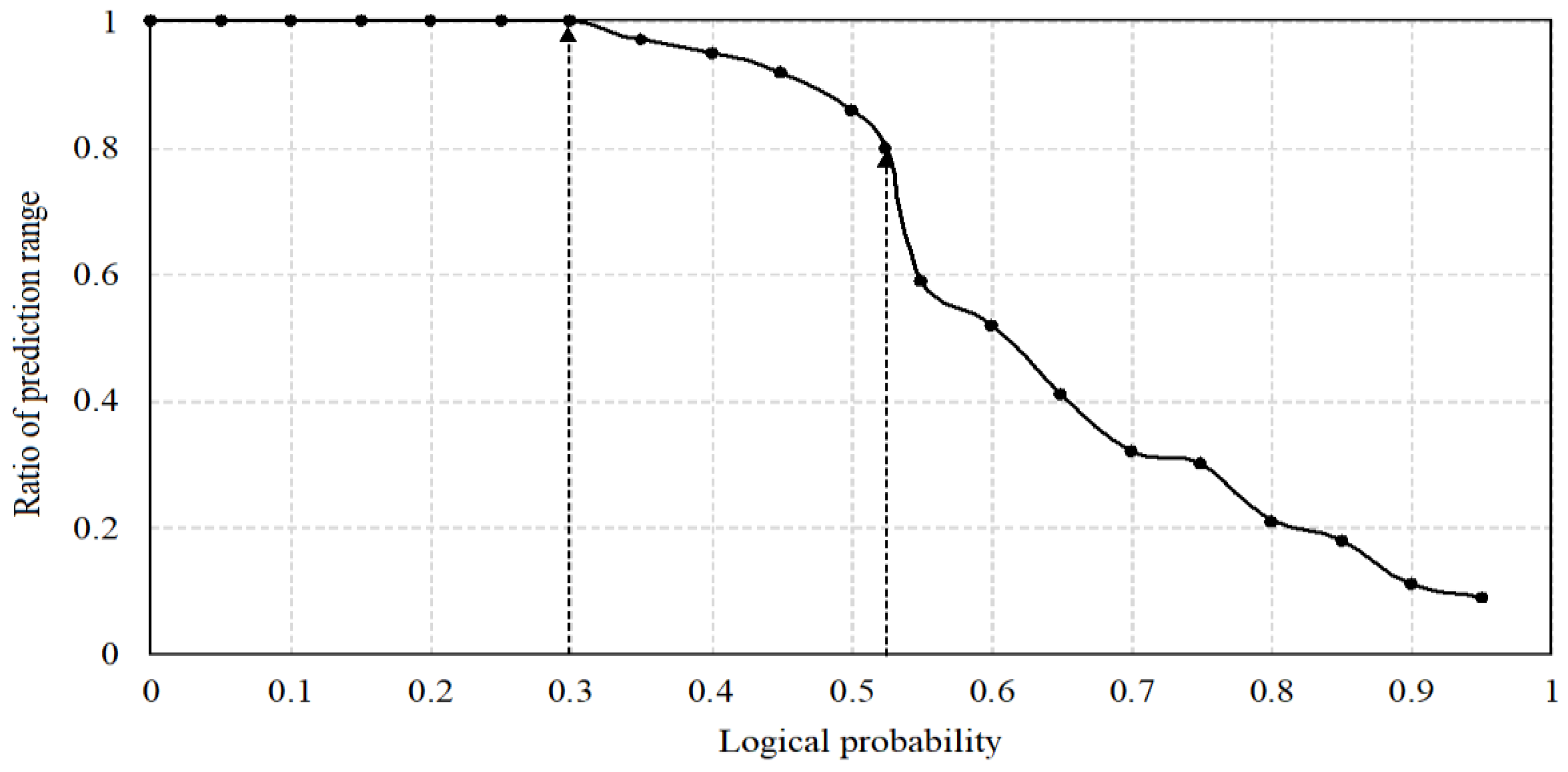
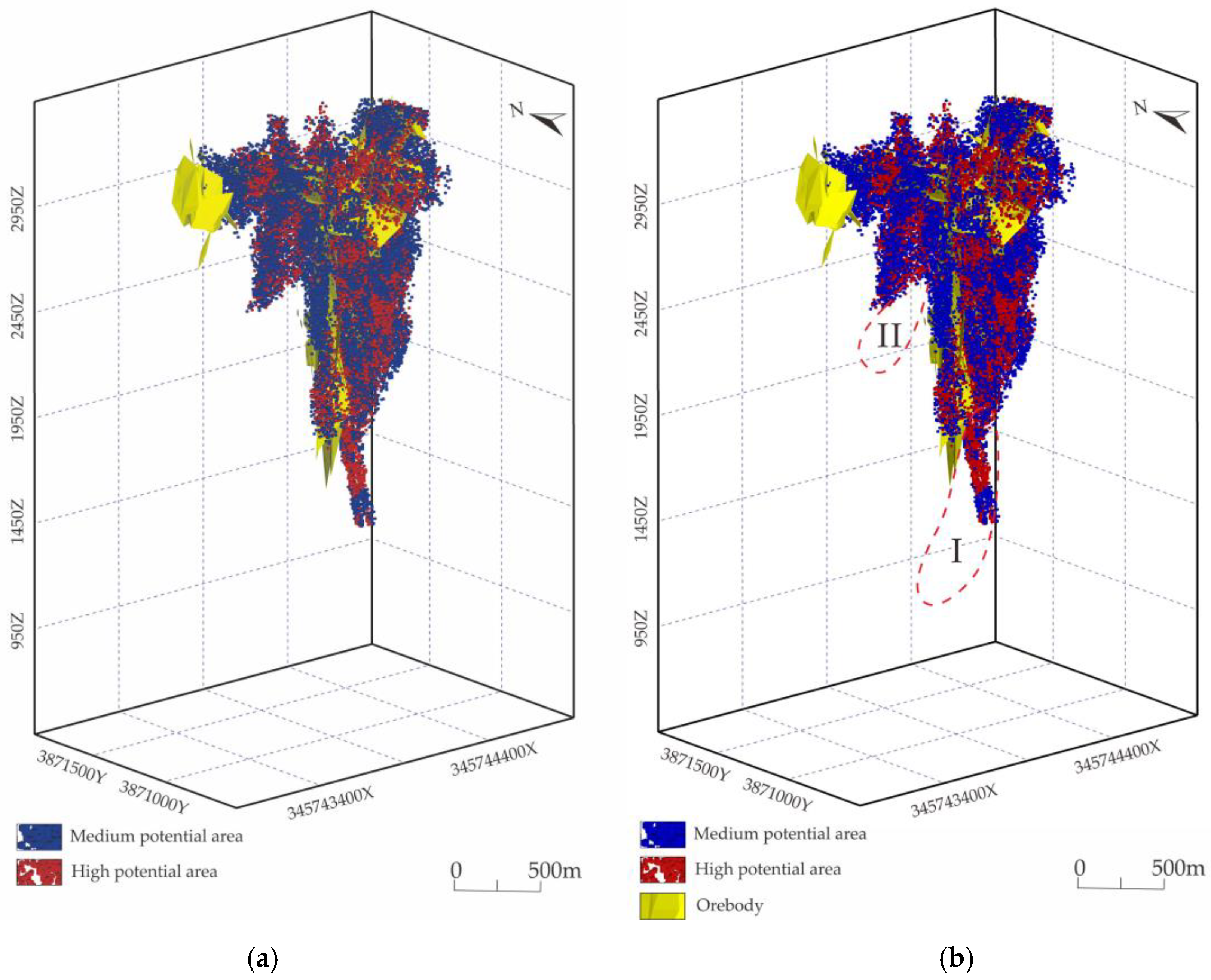
We take the ratio of prediction volume to orebodies occupied volume as a parameter. Observably, it must be that reverse variation of this parameter follows the greater logistic probabilities (Figure 20). The high potential area (logical probability > 0.525) is defined by the logistic probability of 0.525, which covers 80% of the known orebodies; the medium potential area (0.3 < logical probability < 0.525) is defined by the logistic probability of 0.3, which is another inflection point and covers all the known orebodies (Figure 20). The spatial distribution of mineralization potential areas by the MaxEnt model are shown in Figure 21a, based on which two mineral exploration targets are circled (Figure 21b).

4.5.3. Three-Dimensional MPM and Uncertainty Evaluation of GMM

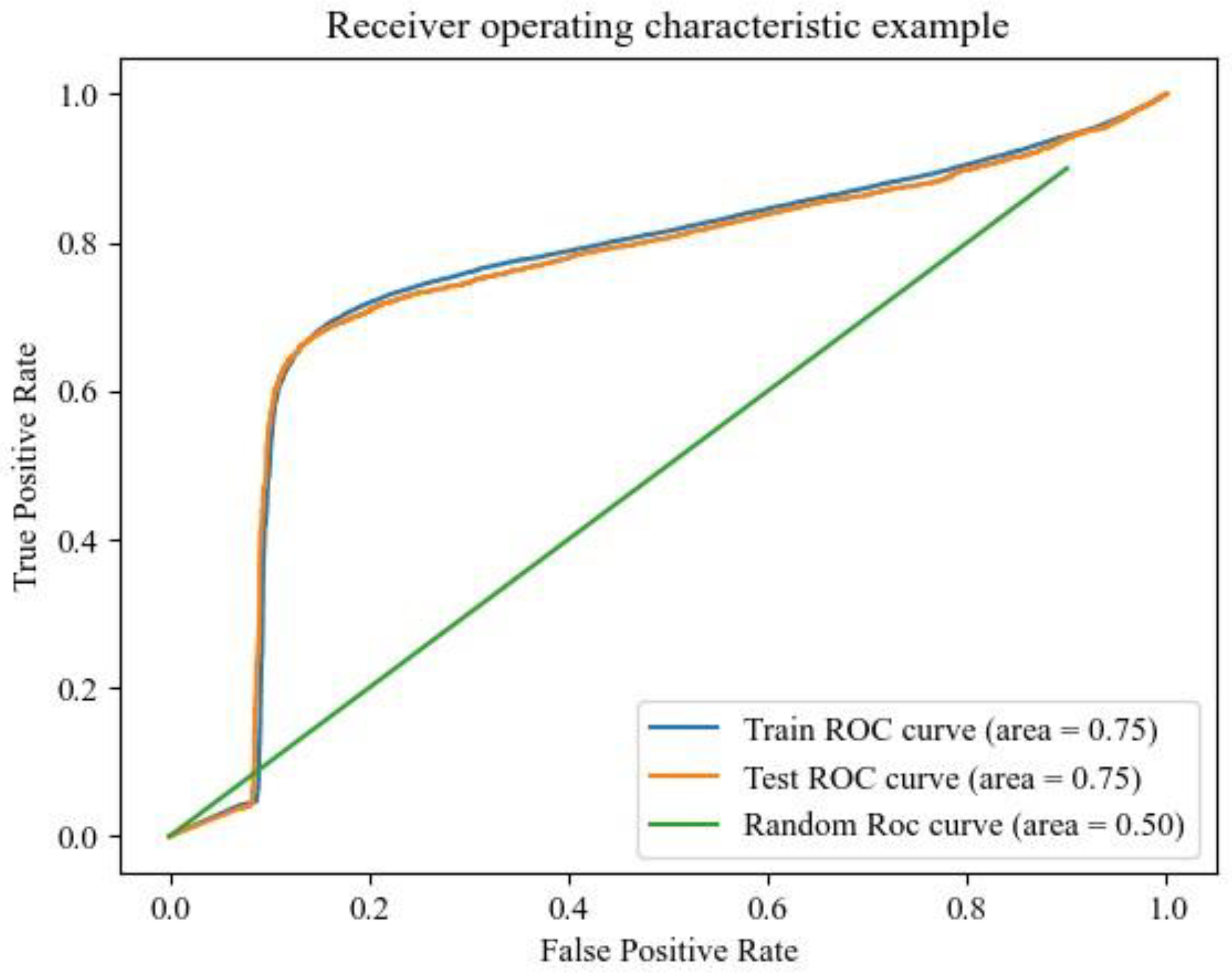
When training and testing the model, the labeled data (which is used only in the evaluation) is divided into 75% for the training dataset and 25% for the test dataset, and the GMM is used to learn the information of the training dataset, and then the ROC curve is used for performance evaluation of the training dataset and test dataset, respectively. The AUC value of the test dataset is 0.75 and the AUC value of the training dataset is 0.75 (Figure 22).
From the point of the AUC value, 0.75 is not a high value, which may indicate that unsupervised training methods have a shortage in prediction with big data.
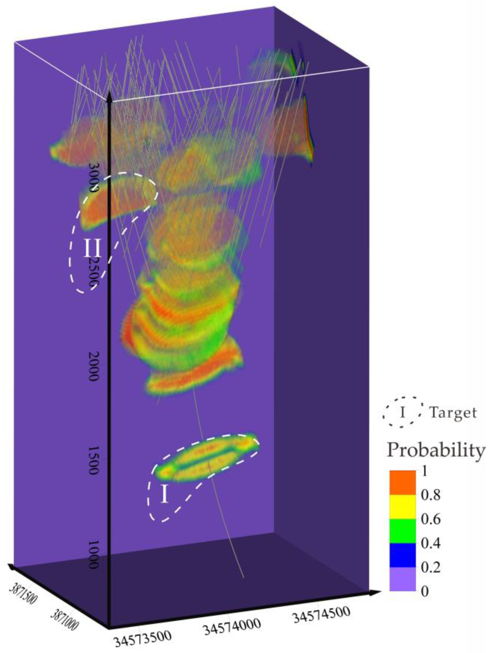
However, from the mineral prospectivity map point of view, the prediction area has covered orebodies well, and it still has a certain indication function in the mineralization prediction. Finally, two mineral exploration targets are delineated at depth (Figure 23).

5. Discussion

This study employed the geostatistical interpolation method to build a 3D geochemical model and geochemical anomaly model. In addition to deterministic modeling of 3D geology and geochemistry [151,152], geostatistical techniques also include uncertainty modeling of spatial distribution of subsurface heterogeneous structures and dynamic processes of fluid migration [153]. In view of the 3D heterogeneous structure, the multi-point geostatistical method can be used to overcome the shortage of traditional geostatistical simulations in delineating the geometric continuity of geological structures [154,155,156,157,158,159]. Meanwhile, traditional geostatistical simulation has the limitations of large computation, complicated parameterization and difficult to characterize multi-scale data. The application of machine learning and deep learning methods to reconstruct geological and geochemical structures can improve the simulation efficiency and can accurately express complex heterogeneous spatial structures [160,161], which deserves further research work.
The machine learning methods of the MaxEnt model and GMM are carried out for 3D MPM in the Zaozigou gold deposit in this study. Compared with the GMM, the MaxEnt model has a higher precision in detection of ore-induced anomalies, which demonstrates a higher reliability of 3D MPM (Figure 18 and Figure 22). The prediction results of the two methods express a high correlation with the known orebodies, based on which two mineral exploration targets are circled (Figure 21 and Figure 23).
Target I of the MaxEnt model is located at an elevation of 1600~2000 m, belonging to the NE-orientation orebody group, which should be the extension of the Au1 orebody. The Au and Sb concentration in this position (Figure 9) and the ratio of front halo to tail halo has been increasing (Figure 16). Additionally, it appears that the high logical probability calculated by the MaxEnt model and GMM at this position indicates the Au1 orebody may extend deeper or a concealed orebody exists therein. Meanwhile, the Target I of GMM is located at the elevation of about 1300 m, reflecting the weak anomaly in the deep drill.
Target II of the two methods is similarly located at the NW-orientation orebody group at the elevation of about 2500 m, where the fractures distribute complexly and the anomalies of tail halo elements and front halo elements overlapped (Figure 9).

6. Conclusions

In this paper, the three-dimensional primary halo anomaly data volume model is built based on the multifractal C-V model, which fully considers the nonlinear characteristics of the primary geochemical data. The C-V model is a three-dimensional extension of the two-dimensional multifractal method, according to which the geochemical concentrations are clearly illustrated at depth. The 3D geochemical anomaly data volume model provides an important element distribution indicator to the 3D MPM.
The data-driven CoDA method was performed in this paper by using clr transformation and factor analysis, among which factor F4 is selected as a prediction indicator. The knowledge-driven CoDA method used the SBP approach to extract the element associations of front halo, near-ore halo and tail halo, and the association of near-ore halo and the ratio of front halo to tail halo are selected as the other two prediction indicators. These selected geochemical association indicators are reliable for their good reflection in metallogenic regularity.
From the results of this paper, the MaxEnt model and the GMM are efficient machine learning methods in 3D MPM. By comparing the spatial distribution of the orebodies and the indication of the metallogenic regularity, the delineated mineral exploration targets can be considered as the mineral potential areas for further investigation. However, it must be mentioned that machine learning algorithms have fast and accurate calculation in the case of small data but lack generalization ability compared with deep learning algorithms in big data. As the amount of data gradually increases, the prediction ability of the MaxEnt model and the GMM usually reach the bottleneck, while deep learning can use more parameters to continuously optimize and improve the detection ability of the models. Deep learning-based 3D Mineral Prospectivity Mapping of the Zaozigou gold deposit should be paid more attention in the further research.

Author Contributions

Ideas, Y.K., G.C. and B.L.; Methodology, Y.K., G.C., C.L. and Z.Y.; software, M.X., S.Z. and H.Z.; writing—original draft preparation, Y.K., G.C., Y.W. and Y.G.; writing—review and editing, G.C. and B.L.; visualization, Y.K., M.X., S.Z., H.Z., L.W. and R.T.; supervision, B.L.; funding acquisition, B.L. All authors have read and agreed to the published version of the manuscript.

Funding

This research was funded by the National Key Research and Development Program of China (Grants 2017YFC0601505); the National Natural Science Foundation of China (Grants 41602334; 42072322); the Key Laboratory of Geochemical Exploration, Ministry of Natural Resources (Grant AS2019P02-01); Sichuan Science and Technology Program (Grant 2022NSFSC0510); and the Opening Fund of the Geomathematics Key Laboratory of Sichuan Province (Grant scsxdz2020yb06, scsxdz2021zd04).

Data Availability Statement

Restrictions apply to the availability of these data. Data was obtained from the Development Research Center of China Geological Survey and No. 3 Geological and Mineral Exploration team, Gansu Provincial Bureau of Geology and Mineral Exploration and Development and are available from Bingli Liu with the permission of the Development Research Center of China Geological Survey and No. 3 Geological and Mineral Exploration team, Gansu Provincial Bureau of Geology and Mineral Exploration and Development.

Acknowledgments

The authors thank the anonymous reviewers and the editors for their hard work on this paper. We are grateful to the Development Research Center of China Geological Survey and No. 3 Geological and Mineral Exploration team, Gansu Provincial Bureau of Geology and Mineral Exploration and Development for their data support.

Conflicts of Interest

The authors declare no conflict of interest.

References

  1. Wang, S.C.; Yang, Y.H.; Yan, G.S.; Li, J.C. Study of large and Giant Gold Deposits: Quantitative Prognosis Method in China. Geol. Rev. 2000, 46, 17–24, (In Chinese with English Abstract). [Google Scholar]
  2. Zhao, P.D. “Three-Component” Quantitative Resource Prediction and Assessments: Theory and Practice of Digital Mineral Prospecting. Earth Sci. 2002, 27, 482–489, (In Chinese with English Abstract). [Google Scholar]
  3. Zhao, P.D. Quantitative mineral prediction and deep mineral exploration. Earth Sci. Front. 2007, 14, 1–10, (In Chinese with English Abstract). [Google Scholar]
  4. Xiao, K.Y.; Zhao, P.D. A Preliminary Discussion on Basic Problems and Researching Programming of the Large Scale Metallogenetic Prognosis. Miner. Explor. 1994, 3, 49–56, (In Chinese with English Abstract). [Google Scholar]
  5. Xiao, K.Y.; Zhang, X.H.; Chen, Z.H.; Song, G.Y.; Ge, Y.; Liu, D.L.; Wang, S.L.; Ning, S.N.; Cao, Y. Comparison of Method of Weights of Evidence and Information. Comput. Tech. Geophys. Geochem. Explor. 1999, 21, 223–226, (In Chinese with English Abstract). [Google Scholar]
  6. Xiao, K.Y.; Zhu, Y.S.; Song, G.Y. Quantitative Evaluation of Mineral Resources GIS. Geol. China. 2000, 278, 29–32. (In Chinese) [Google Scholar]
  7. Xiao, K.Y.; Chen, X.G.; Li, N.; Zou, W.; Sun, L. 3D visualization technology for geological and mineral exploration evaluation and software development for prospectors. Miner. Depos. 2010, 29, 758–760. (In Chinese) [Google Scholar]
  8. Xiao, K.Y.; Li, N.; Sun, L.; Zou, W.; Li, Y. Large scale 3D mineral prediction methods and channels based on 3D information technology. J. Geol. 2012, 36, 229–236, (In Chinese with English Abstract). [Google Scholar]
  9. Xiao, K.Y.; Li, N.; Sun, L.; Zou, W.; Li, Y. 3D Digital Mineral Deposit Model Establishment Method and Its Application. Miner. Deposits 2012, 31, 929–930. (In Chinese) [Google Scholar]
  10. Xiao, K.Y.; Sun, L.; Li, N.; Wang, K.; Fan, J.F.; Ding, J.H. Mineral resources assessment under the thought of big data. Geol. Bull. China 2015, 34, 1266–1272, (In Chinese with English Abstract). [Google Scholar]
  11. Chen, J.P.; Chen, Y.; Zeng, M. 3D positioning and quantitative pre-diction of the Koktokay No. 3 pegmatite dike, Xinjiang, China, based on the digital mineral deposit model. Geol. Bull. China 2008, 27, 552–559, (In Chinese with English Abstract). [Google Scholar]
  12. Chen, J.P.; Lv, P.; Wu, W.; Zhao, J.; Hu, Q. A 3D method for predicting blind orebodies, based on a 3D visualization model and its application. Earth Sci. Front. 2007, 14, 56–65, (In Chinese with English Abstract). [Google Scholar] [CrossRef]
  13. Chen, J.P.; Wang, C.N.; Shang, B.C.; Shi, R. Three-Dimensional Metallogenic Prediction in Yongmei Region Based on Digital Ore Deposit Model. Sci. Technol. Manag. Land Resour. 2012, 29, 14–20, (In Chinese with English Abstract). [Google Scholar]
  14. Chen, J.P.; Yu, M.; Yu, P.P.; Shang, B.C.; Zheng, X.; Wang, L.M. Method and Practice of 3D Geological Modeling at Key Metallogenic Belt with Large and Medium Scale. Acta Geol. Sin. 2014, 88, 1187–1195, (In Chinese with English Abstract). [Google Scholar]
  15. Lv, P. Cube Predicting Model Based 3D Predicting Methods of Blind Orebody and Software Development. Ph.D. Thesis, China University of Geosciences, Beijing, China, 2007. (In Chinese with English Abstract). [Google Scholar]
  16. Zhang, S.H. Deep Learning foe Mineral Prospectivity Mapping of Lala-type Copper Deposit in the Huili Region, Sichuan. Ph.D. Thesis, China University of Geosciences, Beijing, China, 2020. (In Chinese with English Abstract). [Google Scholar]
  17. Zhang, S.H.; Xiao, K.Y. Random Forest—Based Mineralization Prediction of the Lala—Type Cu Deposit in the Huili Area, Sichuan Province. Geol. Explor. 2020, 56, 239–252, (In Chinese with English Abstract). [Google Scholar]
  18. Mao, X.C.; Tang, Y.H.; Deng, H. Three-dimensional morphological analysis method for geologic bodies and its application. J. Cent. South Univ. Sci. Technol. 2012, 43, 588–595, (In Chinese with English Abstract). [Google Scholar]
  19. Mao, X.C.; Tang, Y.H.; Lai, J.Q.; Zou, Y.H.; Chen, J.; Peng, S.L.; Shao, Y.J. Three Dimensional Structure of Metallogenic Geologic Bodies in the Fenghuangshan Ore Field and Ore-controlling Geological Factors. J. Geol. 2011, 85, 1507–1518, (In Chinese with English Abstract). [Google Scholar]
  20. Mao, X.C.; Wang, Q.; Chen, J.; Deng, H.; Liu, Z.K.; Wang, J.L.; Chen, J.P.; Xiao, K.Y. Three-dimensional Modeling of Deep Metallogenic Structure in Northwestern Jiaodong Peninsula and Its Gold Prospecting Significance. Acta Geol. Sin. 2020, 41, 166–178, (In Chinese with English Abstract). [Google Scholar]
  21. Mao, X.C.; Zhang, M.M.; Deng, H.; Zou, Y.H.; Chen, J. 3D Visualization Prediction Method for Concealed Ore Bodies in the Deep. Mining Area. J. Geol. 2016, 40, 363–371, (In Chinese with English Abstract). [Google Scholar]
  22. Mao, X.C.; Zou, Y.H.; Chen, J.; Lai, J.Q.; Peng, S.L.; Shao, Y.J.; Shu, Z.M.; Lv, J.W.; Lv, C.Y. Three-dimensional visual prediction of concealed ore bodies in the deep and marginal parts of crisis mines: A case study of the Fenghuangshan ore field in Tongling, Anhui, China. Geol. Bull. China 2010, 29, 401–413, (In Chinese with English Abstract). [Google Scholar]
  23. Xiang, J.; Chen, J.P.; Xiao, K.Y.; Li, S.; Zhang, Z.P.; Zhang, Y. 3D metallogenic prediction based on machine learning: A case study of the Lala copper deposit in Sichuan Province. Geol. Bull. China 2019, 38, 2010–2021, (In Chinese with English Abstract). [Google Scholar]
  24. Yuan, F.; Li, X.H.; Zhang, M.M.; Jia, C.; Hu, X.Y. Research Progress of 3D Prospectivity Modeling. Gansu Geol. 2018, 27, 32–36, (In Chinese with English Abstract). [Google Scholar]
  25. Yuan, F.; Zhang, M.M.; Li, X.H.; Ge, C.; Lu, S.M.; Li, J.S.; Zhou, Y.Z.; Lan, X.Y. Prospectivity modeling: From two dimension to three-dimension. Acta Petrol. Sin. 2019, 35, 3863–3874, (In Chinese with English Abstract). [Google Scholar]
  26. Cheng, Q.M. What are Mathematical Geosciences and its frontiers? Earth Sci. Front. 2021, 28, 6–25, (In Chinese with English Abstract). [Google Scholar]
  27. Cheng, Q.; Agterberg, F.P.; Ballantyne, S.B. The separation of geochemical anomalies from background by fractal methods. J. Geochem. Explor. 1994, 51, 109–130. [Google Scholar] [CrossRef]
  28. Cheng, Q.M. Multifractality and spatial statistics. Comput. Geosci. 1999, 25, 949–961. [Google Scholar] [CrossRef]
  29. Chen, Z.J.; Cheng, Q.M.; Cheng, J.G.; Xie, S.Y. A novel iterative approach for mapping local singularities from geochemical data. Nonlinear Process. Geophys. 2007, 14, 317–324. [Google Scholar] [CrossRef] [Green Version]
  30. Cheng, Q.M. Modeling local scaling properties for multiscale mapping. Vadose Zone J. 2008, 7, 525–532. [Google Scholar] [CrossRef]
  31. Cheng, Q.M.; Agterberg, F. Multifractals and singularity analysis in mineral exploration and environmental assessment. J. Geochem. Explor. 2018, 189, 1. [Google Scholar] [CrossRef]
  32. Cheng, Q.M. Multifractal and Geostatistic Methods for Characterizing Local Structure and Singularity Properties of Exploration Geochemical Anomalies. Earth Sci. 2001, 26, 161–166, (In Chinese with English Abstract). [Google Scholar]
  33. Carranza, E.J.M. Geochemical Anomaly and Mineral Prospectivity Mapping in GIS. In Handbook of Exploration and Environmental Geochemistry; Elsevier: Amsterdam, The Netherlands, 2009; p. 11. [Google Scholar]
  34. Afzal, P.; Alghalandis, Y.F.; Khakzad, A.; Moarefvand, P.; Omran, N.R. Delineation of mineralization zones in porphyry Cu deposits by fractal concentration–volume modeling. J. Geochem. Explor. 2011, 108, 220–232. [Google Scholar] [CrossRef]
  35. Zuo, R.G.; Wang, J.; Chen, G.X.; Yang, M.G. Identification of weak anomalies: A multifractal perspective. J. Geochem. Explor. 2014, 148, 12–24. [Google Scholar] [CrossRef]
  36. Chen, Y.L. Mineral potential mapping with a restricted Boltzmann machine. Ore Geol. Rev. 2015, 71, 749–760. [Google Scholar] [CrossRef]
  37. Chen, Y.L.; Wu, W. Mapping mineral prospectivity using an extreme learning machine regression. Ore Geol. Rev. 2017, 80, 200–213. [Google Scholar] [CrossRef]
  38. Cheng, Q.M.; Zhang, S.Y.; Zuo, R.G.; Chen, Z.J.; Xie, S.Y.; Xia, Q.L.; Xu, D.Y.; Yao, L.Q. Progress of multifractal filtering techniques and their applications in geochemical information extraction. Earth Sci. Front. 2009, 16, 185–198, (In Chinese with English Abstract). [Google Scholar]
  39. Xiang, Z.L. Study on 3D Geological Modeling method and Prospecting Prediction of Deep Comprehensive Information in Mining area. Ph.D. Thesis, Henan Polytechnic University, JiaoZuo, China, 2019. (In Chinese with English Abstract). [Google Scholar]
  40. Chen, Y.Q.; Zhang, S.Y.; Xia, Q.L.; Li, W.C.; Lu, Y.X.; Huang, J.N. Application of Multi Fractal Filtering to Extraction of Geochemical Anomalies from Multi Geochemical Backgrounds: A Case Study of the Southern Section of “Sanjiang Ore-Forming Zone”, Southwestern China. Earth Sci. 2006, 31, 861–866, (In Chinese with English Abstract). [Google Scholar]
  41. Sun, Z.J. Multifractal Method of Geochem Ical Threshold in Mineral Exploration. Comput. Tech. Geophys. Geochem. Explor. 2007, 29, 54–57+94, (In Chinese with English Abstract). [Google Scholar]
  42. Li, X.H. 3D Prospectivity Modeling for Concealed Orebody and System Development. Ph.D. Thesis, Hefei University Of Technology, Hefei, China, 2015. (In Chinese with English Abstract). [Google Scholar]
  43. Chen, G.X. Identifying Weak But Complex Geophysical and Geochemical Anomalies Caused by Buried Ore Bodies Using Fractal and Wavelet Methods. Ph.D. Thesis, China University of Geosciences, Wuhan, China, 2016. (In Chinese with English Abstract). [Google Scholar]
  44. Liu, S.F. Fractal Analysis on Geochemical Distribution and Anomaly Separation in the Guangxi Zhuang Autonomous Region. Ph.D. Thesis, China University of Geosciences, Beijing, China, 2017. (In Chinese with English Abstract). [Google Scholar]
  45. Carranza, E.J.M.; Zuo, R. Introduction to the thematic issue: Analysis of exploration geochemical data for mapping of anomalies. Geochem. Explor. Env. Anal. 2017, 17, 183–185. [Google Scholar] [CrossRef] [Green Version]
  46. Zuo, R.G.; Cheng, Q.M.; Xia, Q.L. Application of fractal models to characterization of vertical distribution of geochemical element concentration. J. Geochem. Explor. 2009, 102, 37–43. [Google Scholar] [CrossRef]
  47. Delavar, S.T.; Afzal, P.; Borg, G.; Rasa, I.; Lotfi, M.; Omran, N.R. Delineation of mineralization zones using concentration-volume fractal method in Pb-Zn carbonate hosted deposits. J. Geochem. Explor. 2012, 118, 98–110. [Google Scholar] [CrossRef]
  48. Pearson, K. On a Form of Spurious Correlation Which May Arise When Indices Are Used in the Measurement of Organs. Proc. R. Soc. Lond. 1897, 60, 489–502. [Google Scholar]
  49. Chayes, F. On correlation between variables of constant sum. J. Geophys. Res. 1960, 65, 4185–4193. [Google Scholar] [CrossRef]
  50. Egozcue, J.J.; Pawlowsky-Glahn, V. Groups of Parts and Their Balances in Compositional Data Analysis. Math. Geol. 2005, 37, 795–828. [Google Scholar] [CrossRef] [Green Version]
  51. Pawlowsky-Glahn, V.; Egozcue, J.J. Exploring Compositional Data with the CoDa-Dendrogram. Austrian J. Stat. 2011, 40, 103–113. [Google Scholar]
  52. Zhou, D. Geological Compositional Data Analysis: Difficulties and Solutions. Earth Sci. 1998, 23, 41–46, (In Chinese with English Abstract). [Google Scholar]
  53. Carranza, E.J.M. Analysis and mapping of geochemical anomalies using logratio-transformed stream sediment data with censored values. J. Geochem. Explor. 2011, 110, 167–185. [Google Scholar] [CrossRef]
  54. Grunsky, E.C.; Mueller, U.A.; Corrigan, D. A study of the lake sediment geochemistry of the Melville Peninsula using multivariate methods: Applications for predictive geological mapping. J. Geochem. Explor. 2014, 141, 15–41. [Google Scholar] [CrossRef]
  55. Parent, L.E.; Parent, S.T.; Ziadi, N. Biogeochemistry of soil inorganic and organic phosphorus: A compositional analysis with balances. J. Geochem. Explor. 2014, 141, 52–60. [Google Scholar] [CrossRef]
  56. Wang, W.L.; Zhao, J.; Cheng, Q.M. Mapping of Fe mineralization-associated geochemical signatures using logratio transformed stream sediment geochemical data in eastern Tianshan, China. J. Geochem. Explor. 2014, 141, 6–14. [Google Scholar] [CrossRef]
  57. Carranza, E.J.M. Geochemical Mineral Exploration: Should We Use Enrichment Factors or Log-Ratios. Nat. Resour. Res. 2016, 26, 411–428. [Google Scholar] [CrossRef]
  58. Mckinley, J.M.; Grunsky, E.; Mueller, U. Environmental Monitoring and Peat Assessment Using Multivariate Analysis of Regional-Scale Geochemical Data. Math. Geosci. 2017, 50, 235–246. [Google Scholar] [CrossRef] [Green Version]
  59. Reimann, C.; Filzmoser, P.; Hron, K.; Kynlová, P.; Garrett, R.G. A new method for correlation analysis of compositional (environmental) data—A worked example. Sci. Total Environ. 2017, 607, 965–971. [Google Scholar] [CrossRef] [PubMed]
  60. Thiombane, M.; Martín-Fernández, J.; Albanese, S.; Lima, A.; Doherty, A.; Vivo, B.D. Exploratory analysis of multi-element geochemical patterns in soil from the Sarno River Basin (Campania region, southern Italy) through compositional data analysis (CODA). J. Geochem. Explor. 2018, 195, 110–120. [Google Scholar] [CrossRef]
  61. Aitchison, J. The statistical analysis of compositional data. J. R. Stat. Soc. B 1982, 44, 139–177. [Google Scholar] [CrossRef]
  62. Buccianti, A.; Lima, A.; Albanese, S.; Cannatelli, C.; Esposito, R.; Vivo, B.D. Exploring topsoil geochemistry from the CoDA (Compositional Data Analysis) perspective: The multi-element data archive of the Campania Region (Southern Italy). J. Geochem. Explor. 2015, 159, 302–316. [Google Scholar] [CrossRef]
  63. Mckinley, J.M.; Hron, K.; Grunsky, E.C.; Reimann, C.; Tolosana-Delgado, R. The single component geochemical map: Fact or fiction. J. Geochem. Explor. 2016, 162, 16–28. [Google Scholar] [CrossRef] [Green Version]
  64. Buccianti, A.; Lima, A.; Albanese, S.; DeVivo, B. Measuring the change under compositional data analysis (CoDA): Insight on the dynamics of geochemical systems. J. Geochem. Explor. 2018, 189, 100–108. [Google Scholar] [CrossRef]
  65. Liu, Y.; Cheng, Q.M.; Zhou, K.F. New Insights into Element Distribution Patterns in Geochemistry: A Perspective from Fractal Density. Nat. Resour. Res. 2018, 28, 5–29. [Google Scholar] [CrossRef]
  66. Zheng, W.B.; Liu, B.L.; McKinley, J.M.; Cooper, M.R.; Wang, L. Geology and geochemistry-based metallogenic exploration model for the eastern Tethys Himalayan metallogenic belt, Tibet. J. Geochem. Explor. 2021, 224, 106743. [Google Scholar] [CrossRef]
  67. Liu, Y.; Carranza, E.J.M.; Xia, Q. Developments in Quantitative Assessment and Modeling of Mineral Resource Potential: An Overview. Nat. Resour. Res. 2022, 31, 1825–1840. [Google Scholar] [CrossRef]
  68. Agterberg, F. Principles of Probabilistic Regional Mineral Resource Estimation. Earth Sci. 2011, 36, 189–200. [Google Scholar]
  69. Zhou, Y.Z.; Chen, S.; Zhang, Q.; Xiao, F.; Wang, S.G.; Liu, Y.P.; Jiao, S.T. Advances and Prospects of Big Data and Mathematical Geoscience. Acta Petrol. Sin. 2018, 34, 255–263, (In Chinese with English Abstract). [Google Scholar]
  70. Zhou, Y.Z.; Wang, J.; Zuo, R.G.; Xiao, F.; Shen, W.J.; Wang, S.G. Machine learning, deep learning and Python language in field of geology. Acta Petrol. Sin. 2018, 34, 3173–3178, (In Chinese with English Abstract). [Google Scholar]
  71. Zhou, Y.Z.; Zuo, R.G.; Liu, G.; Yuan, F.; Mao, X.C.; Guo, Y.J.; Liao, J.; Liu, Y.P. The Great-leap-forward Development of Mathematical Geoscience During 2010–2019: Big Data and Artificial Intelligence Algorithm Are Changing Mathematical Geoscience. Bull. Miner. Petrol. Geochem. 2021, 40, 556–573+777, (In Chinese with English Abstract). [Google Scholar]
  72. Zuo, R.G. Deep Learning-Based Mining and Integration of Deep-Level Mineralization Information. Bull. Miner. Petrol. Geochem. 2019, 38, 53–60, (In Chinese with English Abstract). [Google Scholar]
  73. Zuo, R.G.; Peng, Y.; Li, T.; Xiong, Y.H. Challenges of Geological Prospecting Big Data Mining and Integration Using Deep Learning Algorithms. Earth Sci. 2021, 46, 350–358, (In Chinese with English Abstract). [Google Scholar]
  74. Zuo, R.G.; Carranza, E.J.M. Support vector machine: A tool for mapping mineral prospectivity. Comput. Geosci. 2011, 37, 1967–1975. [Google Scholar] [CrossRef]
  75. Shabankareh, M.; Hezarkhani, A. Application of support vector machines for copper potential mapping in Kerman region, Iran. J. Afr. Earth Sci. 2016, 128, 116–126. [Google Scholar] [CrossRef]
  76. Zhang, S.; Xiao, K.Y.; Carranza, E.J.M.; Yang, F. Maximum Entropy and Random Forest Modeling of Mineral Potential: Analysis of Gold Prospectivity in the Hezuo–Meiwu District, West Qinling Orogen, China. Nat. Resour. Res. 2018, 28, 645–664. [Google Scholar] [CrossRef]
  77. Sun, T.; Chen, F.; Zhong, L.X.; Liu, W.M.; Wang, Y. GIS-based mineral prospectivity mapping using machine learning methods: A case study from Tongling ore district, eastern China. Ore Geol. Rev. 2019, 109, 26–49. [Google Scholar] [CrossRef]
  78. Wang, J.; Zuo, R.G.; Xiong, Y.H. Mapping Mineral Prospectivity via Semi-supervised Random Forest. Nat. Resour. Res. 2019, 29, 189–202. [Google Scholar] [CrossRef]
  79. Sun, T.; Li, H.; Wu, K.X.; Chen, F.; Hu, Z.J. Data-Driven Predictive Modelling of Mineral Prospectivity Using Machine Learning and Deep Learning Methods: A Case Study from Southern Jiangxi Province, China. Minerals 2020, 10, 102. [Google Scholar] [CrossRef] [Green Version]
  80. Wang, Z.Y.; Zuo, R.G.; Dong, Y.N. Mapping Himalayan leucogranites using a hybrid method of metric learning and support vector machine. Comput. Geosci. 2020, 138, 104455. [Google Scholar] [CrossRef]
  81. Chen, J.; Mao, X.C.; Liu, Z.K.; Deng, H. Three-dimensional Metallogenic Prediction Based on Random Forest Classification Algorithm for the Dayingezhuang Gold Deposit. Geotecton. Metallog. 2020, 44, 231–241, (In Chinese with English Abstract). [Google Scholar]
  82. Li, C.B.; Xiao, K.Y.; Li, N.; Song, X.L.; Zhang, S.; Wang, K.; Chu, W.K.; Cao, R. A Comparative Study of Support Vector Machine, Random Forest and Artificial Neural Network Machine Learning Algorithms in Geochemical Anomaly Information Extraction. Acta Geosci. Sin. 2020, 41, 309–319, (In Chinese with English Abstract). [Google Scholar]
  83. Wang, Y.; Zhou, Y.Z.; Xiao, F.; Wang, J.; Wang, K.Q.; Yu, X.T. Numerical Metallogenic Modelling and Support Vector Machine Methods Applied to Predict Deep Mineralization: A Case Study from the Fankou Pb-Zn Ore Deposit in Northern Guangdong. Geotecton. Metallog. 2020, 44, 222–230, (In Chinese with English Abstract). [Google Scholar]
  84. Li, S.; Chen, J.P.; Liu, C.; Wang, Y. Mineral Prospectivity Prediction via Convolutional Neural Networks Based on Geological Big Data. J. Earth Sci. 2021, 32, 327–347. [Google Scholar] [CrossRef]
  85. Zhang, S.; Carranza, E.J.M.; Wei, H.T.; Xiao, K.Y.; Yang, F.; Xiang, J.; Zhang, S.H.; Xu, Y. Data-driven Mineral Prospectivity Mapping by Joint Application of Unsupervised Convolutional Auto-encoder Network and Supervised Convolutional Neural Network. Nat. Resour. Res. 2021, 30, 1011–1031. [Google Scholar] [CrossRef]
  86. Zhou, Y.Z.; Li, P.X.; Wang, S.G.; Xiao, F.; Li, J.Z.; Gao, L. Research Progress on Big Data and Intelligent Modelling of Mineral Deposits. Bull. Miner. Petrol. Geochem. 2017, 36, 327–331+344, (In Chinese with English Abstract). [Google Scholar]
  87. Singer, D.A.; Kouda, R. Application of a feed forward neural network in the search for Kuroko deposits in the Hokuroku District. Math. Geol. 1996, 28, 1017–1023. [Google Scholar] [CrossRef]
  88. Rodriguez-Galiano, V.; Sanchez-Castillo, M.; Chica-Olmo, M.; Chica-Rivas, M. Machine learning predictive models for mineral prospectivity: An evaluation of neural networks, random forest, regression trees and support vector machines. Ore Geol. Rev. 2015, 71, 804–818. [Google Scholar] [CrossRef]
  89. Zuo, R.G.; Xiong, Y.H. Geodata science and geochemical mapping. J. Geochem. Explor. 2019, 209, 106431. [Google Scholar] [CrossRef]
  90. Xiong, Y.H.; Zuo, R.G. Robust Feature Extraction for Geochemical Anomaly Recognition Using a Stacked Convolutional Denoising Autoencoder. Math. Geosci. 2021, 54, 623–644. [Google Scholar] [CrossRef]
  91. Gao, Y. Mineral Prospecting Information Mining and Mapping Mineral Prospectivity for Copper Polymetallic Mineralization in Southwest Fujian Province, China. Ph.D. Thesis, China University of Geosciences, Wuhan, China, 2019. (In Chinese with English Abstract). [Google Scholar]
  92. Zuo, R.G. Geodata Science-Based Mineral Prospectivity Mapping: A Review. Nat. Resour. Res. 2020, 29, 3415–3424. [Google Scholar] [CrossRef]
  93. Li, T.; Zuo, R.G.; Xiong, Y.H.; Peng, Y. Random-Drop Data Augmentation of Deep Convolutional Neural Network for Mineral Prospectivity Mapping. Nat. Resour. Res. 2020, 30, 27–38. [Google Scholar] [CrossRef]
  94. Cai, H.H.; Xu, Y.Y.; Li, Z.X.; Cao, H.H.; Feng, Y.X.; Chen, S.Q.; Li, Y.S. The division of metallogenic prospective areas based onconvolutional neural network model: A case study of the Daqiao gold polymetallic deposit. Geol. Bull. China 2019, 38, 1999–2009, (In Chinese with English Abstract). [Google Scholar]
  95. Wang, Z.Y. Mapping of Himalaya Leucogranites Based on Metric Learning. Ph.D. Thesis, China University of Geosciences, Wuhan, China, 2020. (In Chinese with English Abstract). [Google Scholar]
  96. Deng, H.; Wei, Y.F.; Chen, J.; Liu, Z.K.; Yu, S.Y.; Mao, X.C. Three-dimensional prospectivity mapping and quantitative analysis of structural ore-controlling factors in Jiaojia Auore-belt with attention convolutional neural networks. J. Cent. South Univ. 2021, 52, 3003–3014, (In Chinese with English Abstract). [Google Scholar]
  97. Deng, H.; Zheng, Y.; Chen, J.; Wei, Y.F.; Mao, X.C. Deep Learning-based 3D Prediction Model for the Dayingezhuang Gold Deposit, Shandong Province. Acta Geosci. Sin. 2020, 41, 157–165, (In Chinese with English Abstract). [Google Scholar]
  98. Zhang, Z.J.; Cheng, Q.M.; Yang, J.; Wu, G.P.; Ge, Y.Z. Machine Learning for Mineral Prospectivity: A Case Study of Iron-polymetallic Mineral Prospectivity in Southwestern Fujian. Earth Sci. Front. 2021, 28, 221–235, (In Chinese with English Abstract). [Google Scholar]
  99. Feng, Y.M.; Cao, X.Z.; Zhang, E.P.; Hu, Y.X.; Pan, X.P.; Yang, J.L.; Jia, Q.Z.; Li, W.M. Tectonic Evolution Framework and Nature of The West Qinling Orogenic Belt. Northwest. Geol. 2003, 36, 1–10, (In Chinese with English Abstract). [Google Scholar]
  100. Wei, L.X. Tectonic Evolution and Mineralization of Zaozigou Gold Deposit, Gansu Province. Master’s Thesis, China University of Geosciences, Beijing, China, 2015. (In Chinese with English Abstract). [Google Scholar]
  101. Zeng, J.J.; Li, K.N.; Yan, K.; Wei, L.L.; Huo, X.D.; Zhang, J.P. Tectonic Setting and Provenance characteristics of the Lower Triassic Jiangligou Formation in West Qinling—Constraints from Geochemistry of Clastic Rock and zircon U-Pb Geochronology of Detrital Zircon. Geol. Rev. 2021, 67, 1–15, (In Chinese with English Abstract). [Google Scholar]
  102. Li, Z.B.; Liu, Z.Y.; Li, R. Geochemical Characteristics and metallogenic Potential Analysis of Daheba Formation in Ta-Ga Area of Gansu Province. Contrib. Geol. Miner. Resour. Res. 2021, 36, 187–194, (In Chinese with English Abstract). [Google Scholar]
  103. Chen, Y.; Wang, K.J. Geological Features and Ore Prospecting Indicators of Sishangou Silver Deposit. Gansu. Metal. 2015, 37, 108–111, (In Chinese with English Abstract). [Google Scholar]
  104. Di, P.F. Geochemistry and Ore-Forming Mechanism on Zaozigou gold deposit in Xiahe-Hezuo, West Qinling, China. Ph.D. Thesis, Lanzhou University, Lanzhou, China, 2018. (In Chinese with English Abstract). [Google Scholar]
  105. Li, K.N.; Li, H.R.; Liu, B.C.; Yan, K.; Jia, R.Y.; Wei, L.L. Geochemical characteristics of TTG Dick rock and the Relation with Gold Mineralization in West Qinling Mountain. Sci. Technol. Eng. 2019, 19, 52–65, (In Chinese with English Abstract). [Google Scholar]
  106. Kang, S.S. Geological Characteristics and Prospecting Criteria of Nanmougou Copper Deposit, Gansu Province. Gansu. Metal. 2018, 40, 79–85, (In Chinese with English Abstract). [Google Scholar]
  107. Kang, S.S.; Dou, X.G.; Zhi, C.; Wu, X.L. Geochemical Characteristics and Genetic Analysis of the Namugou Copper Deposit in Sunan County, Gansu. Gansu. Metal. 2019, 41, 65–72, (In Chinese with English Abstract). [Google Scholar]
  108. Liu, Y. Relationship between Intermediate-acid Dike Rock and Gold Mineralization of the Zaozigou Deposit, Gansu Province. Master’s Thesis, Chang’an University, Xi’an, China, 2013. (In Chinese with English Abstract). [Google Scholar]
  109. Hu, J.Q. Mineral Control Factors, Metallogenic Law and Prospecting Direction of Integrated Gold Mine Exploration Area in Shilijba-Yangshan Area of Gansu Province. Gansu. Sci. Technol. 2018, 34, 27–33. (In Chinese) [Google Scholar]
  110. Zhao, J.Z.; Chen, G.Z.; Liang, Z.L.; Zhao, J.C. Ore-body Geochemical Features of Zaozigou Gold Deposit. Gansu. Geol. 2013, 22, 38–43, (In Chinese with English Abstract). [Google Scholar]
  111. Lu, J. Study on Characteristics and Ore-host Regularity of Gold Mineral in the Western Qinling Region, Gansu Province. Master’s Thesis, China University of Geosciences, Beijing, China, 2016. (In Chinese with English Abstract). [Google Scholar]
  112. Zhang, Y.N.; Liang, Z.L.; Qiu, K.F.; Ma, S.H.; Wang, J.L. Overview on the Metallogenesis of Zaozigou gold deposit in the West Qinling Orogen. Miner. Explor. 2020, 11, 28–39, (In Chinese with English Abstract). [Google Scholar]
  113. Tang, L.; Lin, C.G.; Cheng, Z.Z.; Jia, R.Y.; Li, H.R.; Li, K.N. 3D Characteristics of Primary Halo and Deep Prospecting Prediction in The Zaozigou Gold Deposit, Hezuo City, Gansu Province. Geol. Bull. China 2020, 39, 1173–1181, (In Chinese with English Abstract). [Google Scholar]
  114. Chen, G.Z.; Wang, J.L.; Liang, Z.L.; Li, P.B.; Ma, H.S.; Zhang, Y.N. Analysis of Geological Structures in Zaozigou Gold Deposit of Gansu Province. Gansu. Geol. 2013, 22, 50–57, (In Chinese with English Abstract). [Google Scholar]
  115. Chen, G.Z.; Liang, M.L.; Wang, J.L.; Zhang, Y.N.; Li, P.B. Characteristics and Deep Prediction of Primary Superimposed Halos in The Zaozigou Gold Deposit of Hezuo, Gansu Province. Geophys. Geochem. Explor. 2014, 38, 268–277, (In Chinese with English Abstract). [Google Scholar]
  116. Jin, D.G.; Liu, B.C.; Chen, Y.Y.; Liang, Z.L. Spatial Distribution of Gold Bodies in Zaozigou Mine of Gansu Province. Gansu. Geol. 2015, 24, 25–30+41, (In Chinese with English Abstract). [Google Scholar]
  117. Zhu, F.; Wang, G.W. Study on Grade Model of Gansu Zaozigou Gold Mine Based on Geological Statistics. Acta Mineral. Sin. 2015, 35, 1065–1066. (In Chinese) [Google Scholar]
  118. Chen, G.Z.; Li, L.N.; Zhang, Y.N.; Ma, H.S.; Liang, Z.L.; Wu, X.M. Characteristics of fluid inclusions and deposit formation in Zaozigou gold mine. In Proceedings of the The 15th Annual Academic Conference of Chinese Society for Mineralogy, Petrology and Geochemistry, Changchun, China, 24 June 2015. [Google Scholar]
  119. Wu, X.M. Study on Geological Characteristics and Metallogenic Regularity of the Gelouang Gold Deposit. Master’s Thesis, Lanzhou University, Lanzhou, China, 2018. (In Chinese with English Abstract). [Google Scholar]
  120. Liu, H.T.; Jiang, Y.M.; Wu, T.J.; Chang, D.L. Application of singularity analysis to geochemical anomaly recognization in Chifeng area. Contrib. Geol. Miner. Resour. Res. 2011, 26, 341–344, (In Chinese with English Abstract). [Google Scholar]
  121. Wang, Y. The Application of Fractal Theory in Geophysical Research. Master’s Thesis, Chang’an University, Xi’an, China, 2013. (In Chinese with English Abstract). [Google Scholar]
  122. Filzmoser, P.; Hron, K.; Reimann, C. Univariate statistical analysis of environmental (compositional) data: Problems and possibilities. Sci. Total Environ. 2009, 407, 6100–6108. [Google Scholar] [CrossRef]
  123. Wang, L.; Liu, B.L.; McKinley, J.M.; Cooper, M.R.; Li, C.; Kong, Y.H.; Shan, M.X. Compositional data analysis of regional geochemical data in the Lhasa area of Tibet, China. Appl. Geochem. 2021, 135, 105108. [Google Scholar] [CrossRef]
  124. Zheng, W.B.; Liu, B.L.; Tang, J.X.; McKinley, J.M.; Cooper, M.R.; Tang, P.; Lin, B.; Li, C.; Wang, L.; Zhang, D. Exploration indicators of the Jiama porphyry–skarn deposit, southern Tibet, China. J. Geochem. Explor. 2022, 236, 106982. [Google Scholar] [CrossRef]
  125. Zuo, R.G. Identification of weak geochemical anomalies using robust neighborhood statistics coupled with GIS in covered areas. J. Geochem. Explor. 2014, 136, 93–101. [Google Scholar] [CrossRef]
  126. Liu, Y. The Study of Regional Geochemistry Data Analysis and Metallogenic Information Fusion Models. Ph.D. Thesis, China University of Geosciences, Wuhan, China, 2015. (In Chinese with English Abstract). [Google Scholar]
  127. Prado, E.; Filho, C.; Carranza, E.; Motta, J.G. Modeling of Cu-Au Prospectivity in the Carajás mineral province (Brazil) through Machine Learning: Dealing with Imbalanced Training Data. Ore Geol. Rev. 2020, 124, 103611. [Google Scholar] [CrossRef]
  128. Brown, W.M.; Gedeon, T.D.; Groves, D.I.; Barnes, R.G. Artificial neural networks: A new method for mineral prospectivity mapping. Aust. J. Earth Sci. 2000, 47, 757–770. [Google Scholar] [CrossRef]
  129. Skabar, A. Mineral potential mapping using feed-forward neural networks. In Proceedings of the International Joint Conference on Neural Networks IEEE, Portland, OR, USA, 20–24 July 2003. [Google Scholar]
  130. Leite, E.P.; Filho, C. Probabilistic neural networks applied to mineral potential mapping for platinum group elements in the Serra Leste region, Carajás Mineral Province, Brazil. Comput. Geosci. 2009, 35, 675–687. [Google Scholar] [CrossRef]
  131. Leite, E.P.; de Souza, C.R. Artificial neural networks applied to mineral potential mapping for copper-gold mineralizations in the Carajás Mineral Province, Brazil. Geophys. Prospect. 2009, 57, 1049–1065. [Google Scholar] [CrossRef]
  132. Abedi, M.; Norouzi, G.H.; Bahroudi, A. Support vector machine for multi-classification of mineral prospectivity areas. Comput. Geosci. 2012, 9, 272–283. [Google Scholar] [CrossRef]
  133. Rodriguez-Galiano, V.F.; Chica-Olmo, M.; Chica-Rivas, M. Predictive modelling of gold potential with the integration of multisource information based on random forest: A case study on the Rodalquilar area, Southern Spain. Int. J. Geogr. Inf. Sci. 2014, 28, 1336–1354. [Google Scholar] [CrossRef]
  134. Gao, Y.; Zhang, Z.J.; Xiong, Y.H.; Zuo, R.G. Mapping mineral prospectivity for Cu polymetallic mineralization in southwest Fujian Province, China. Ore Geol. Rev. 2016, 75, 16–28. [Google Scholar] [CrossRef]
  135. Geranian, H.; Tabatabaei, S.H.; Asadi, H.H.; Carranza, E.J.M. Application of Discriminant Analysis and Support Vector Machine in Mapping Gold Potential Areas for Further Drilling in the Sari-Gunay Gold Deposit, NW Iran. Nat. Resour. Res. 2016, 25, 145–159. [Google Scholar] [CrossRef]
  136. Xie, S. Research on the prediction of potential suitable distribution of Biomphalaria straminea in Guangdong Province. Master’s Thesis, South China Agricultural University, Guangzhou, China, 2017. (In Chinese with English Abstract). [Google Scholar]
  137. Xu, C. Distribution of Vehicle Free Flow Speeds Based on Gaussian Mixture Model. J. Highw. Transp. Res. Dev. Chin. Ed. 2012, 19, 132–158, (In Chinese with English Abstract). [Google Scholar]
  138. Matheron, G. Kriging or polynomial interpolation procedures? Trans. Can. Inst. Min. Metal. 1967, 70, 240–244. [Google Scholar]
  139. Journel, A.G.; Huijbregts, C.J. Mining Geostatistics; Academic Press: London, UK, 1978. [Google Scholar]
  140. Cressie, N. The origins of kriging. Math. Geosci. 1990, 22, 239–252. [Google Scholar] [CrossRef]
  141. Wang, H.; Lineweaver, C.H. Chemical Complementarity between the Gas Phase of the Interstellar Medium and the Rocky Material of Our Planetary System. In Proceedings of the 15th Australian Space Research Conference, Canberra, Australia, 29 September–1 October 2016; pp. 173–182. [Google Scholar]
  142. Ye, T.Z. Theoretical Framework of Synthetic Geological Information Prediction Techniques and Methods for Mineral Deposit Models. J. Jilin Univ. Earth Sci. Ed. 2013, 43, 1053–1072, (In Chinese with English Abstract). [Google Scholar]
  143. Beus, A.A.; Grigorian, S.V. Geochemical Exploration Methods for Mineral Deposits; Applied Publishing Ltd.: Wilmette, IL, USA, 1977; pp. 31–270. [Google Scholar]
  144. Levinson, A.A. Introduction to Exploration Geochemistry; Applied Publishing Ltd.: Wilmette, IL, USA, 1974; p. 612. [Google Scholar]
  145. Rabeaut, O.; Legault, M.; Cheilletz, A.; Jébrak, M.; Royer, J.J.; Cheng, L.Z. Gold Potential of a Hidden Archean Fault Zone: The Case of the Cadillac–Larder Lake Fault. Explor. Min. Geol. 2010, 19, 99–116. [Google Scholar] [CrossRef]
  146. Mejia-Herrera, P.; Royer, J.J.; Caumon, G.; Cheilletz, A. Curvature Attribute from Surface-Restoration as Predictor Variable in Kupferschiefer Copper Potentials: An Example from the Fore-Sudetic Region. Nat. Resour. Res. 2015, 24, 275–290. [Google Scholar] [CrossRef]
  147. Li, B.B.; Liu, B.L.; Guo, K.; Li, C.; Wang, B. Application of a Maximum Entropy Model for Mineral Prospectivity Maps. Minerals 2019, 9, 556. [Google Scholar] [CrossRef] [Green Version]
  148. Kong, W.X.; Li, X.H.; Zou, H.F. Optimization of Maximum Entropy Model in Species Distribution Prediction. J. Appl. Ecol. 2019, 30, 2116–2128, (In Chinese with English Abstract). [Google Scholar]
  149. Elith, J.; Phillips, S.J.; Hastie, T.; Dudik, M.; Chee, Y.E.; Yates, C.J. A statistical explanation of MaxEnt for ecologists. Divers. Distrib. 2013, 17, 43–57. [Google Scholar] [CrossRef]
  150. Radosavljevic, A.; Anderson, R.P. Making better MAXENT models of species distributions: Complexity, overfitting and evaluation. J. Biogeogr. 2013, 41, 629–643. [Google Scholar] [CrossRef]
  151. Caumon, G.; Collon-Drouaillet, P.; De Veslud, C.L.C.; Viseur, S.; Sausse, J. Surface-based 3D modeling of geological structures. Math. Geosci. 2009, 41, 927–945. [Google Scholar] [CrossRef] [Green Version]
  152. Chen, Q.; Liu, G.; Li, X.; Zhang, Z.; Li, Y. A corner-point-grid-based voxelization method for the complex geological structure model with folds. J. Vis. 2017, 20, 875–888. [Google Scholar] [CrossRef]
  153. Yarus, J.M.; Chambers, R.L. Stochastic Modeling and Geostatistics: Principles, Methods, and Case Studies; American Association of Petroleum Geologists: Tulsa, OK, USA, 1994; p. 379. [Google Scholar]
  154. Chen, Q.; Liu, G.; Ma, X.; Li, X.; He, Z. 3D stochastic modeling framework for Quaternary sediments using multiple-point statistics: A case study in Minjiang Estuary area, southeast China. Comput. Geosci. 2019, 136, 104404. [Google Scholar] [CrossRef]
  155. Chen, Q.; Mariethoz, G.; Liu, G.; Comunian, A.; Ma, X. Locality-based 3-D multiple-point statistics reconstruction using 2-D geological cross sections. Hydrol. Earth Syst. Sci. 2018, 22, 6547–6566. [Google Scholar] [CrossRef] [Green Version]
  156. Gueting, N.; Caers, J.; Comunian, A.; Vanderborght, J.; Englert, A. Reconstruction of three-dimensional aquifer heterogeneity from two-dimensional geophysical data. Math. Geosci. 2018, 50, 53–75. [Google Scholar] [CrossRef] [Green Version]
  157. Mahmud, K.; Mariethoz, G.; Baker, A.; Treble, P.C. Hydrological characterization of cave drip waters in a porous limestone: Golgotha Cave, Western Australia. Hydrol. Earth Syst. Sci. 2018, 22, 977–988. [Google Scholar] [CrossRef] [Green Version]
  158. Feng, W.; Yin, Y.; Zhang, C.; Duan, T.; Zhang, W.; Hou, G.; Zhao, L. A training image optimal selecting method based on composite correlation coefficient ranking for multiple-point geostatistics. J. Petrol. Sci. Eng. 2019, 179, 292–311. [Google Scholar] [CrossRef]
  159. Cui, Z.; Chen, Q.; Liu, G.; Mariethoz, G.; Ma, X. Hybrid parallel framework for multiple-point geostatistics on tianhe-2: A robust solution for large-scale simulation. Comput. Geosci. 2021, 157, 104923. [Google Scholar] [CrossRef]
  160. Chen, Q.; Cui, Z.; Liu, G.; Yang, Z.; Ma, X. Deep convolutional generative adversarial networks for modeling complex hydrological structures in Monte-Carlo simulation. J. Hydrol. 2022, 610, 127970. [Google Scholar] [CrossRef]
  161. Yang, Z.; Chen, Q.; Cui, Z.; Liu, G.; Dong, S.; Tian, Y. Automatic reconstruction method of 3D geological models based on deep convolutional generative adversarial networks. Comput. Geosci. 2022, 26, 1135–1150. [Google Scholar] [CrossRef]
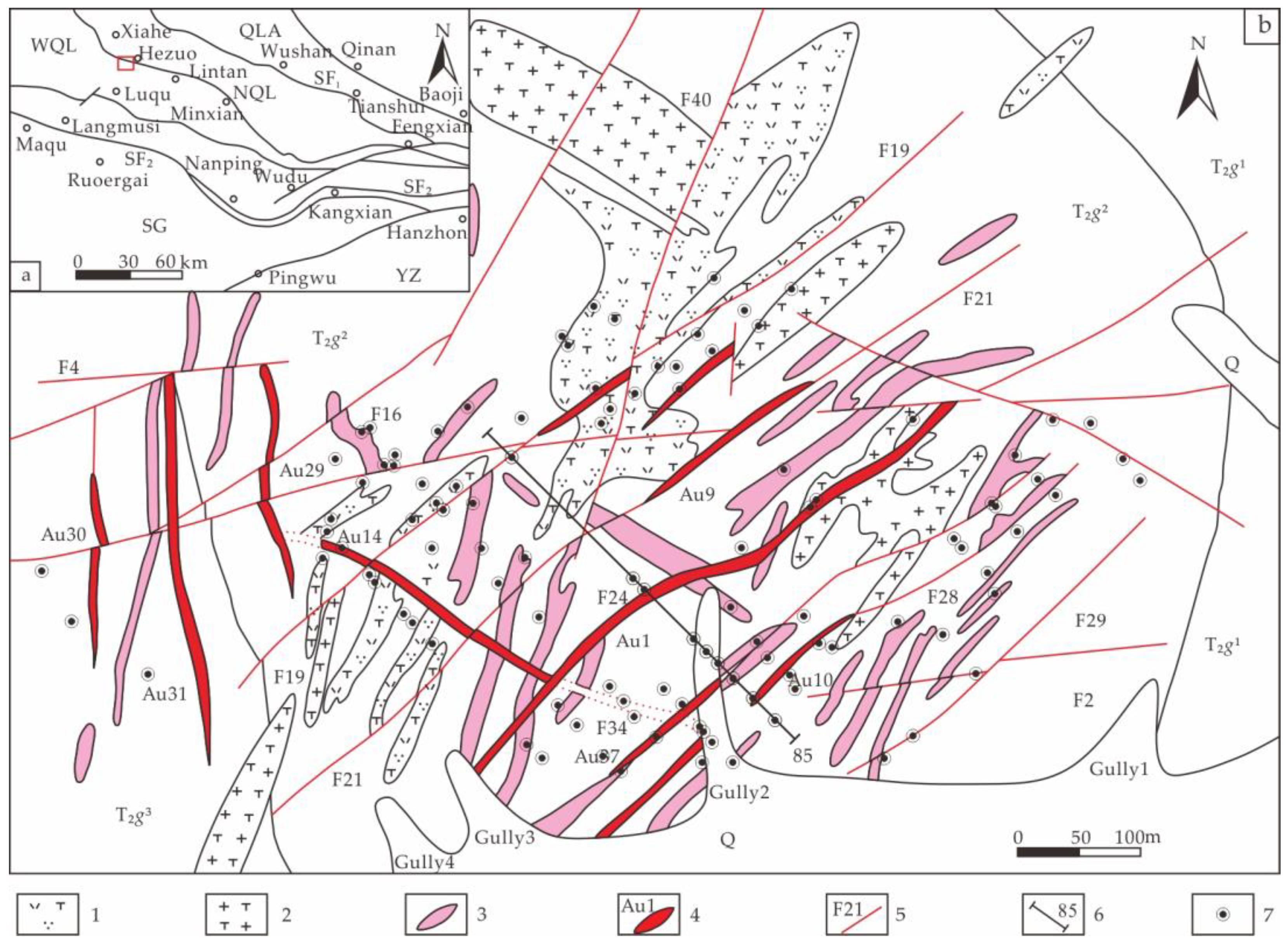
Figure 2. (a) Regional location of study area. QLA = Qilian tectonic belt; WQL: West Qinling tectonic belt; NQL: North Qaidam tectonic belt; SF1: Wushan–Tianshui–Shangdan suture zone; SF2: Maqu–Nanping–Lueyang suture zone; SG: Songpan–Ganzi tectonic belt; YZ: Yangtze block. (b) Geological map of Zaozigou gold deposit (modified from [113]). 1. Quartz diorite porphyrite; 2. Granodiorite-porphyry; 3. Plagioclase granite porphyry; 4. Gold orebody; 5. Fracture; 6. Mineral exploration line; 7. Drilling Hole.
Minerals 12 01361 g002
Figure 3. 3D model of Drillings in Zaozigou gold deposit. (a) Plan view of drillings distribution. (b) Side view of drillings distribution. (c) Sample grade distribution of drillings.
Minerals 12 01361 g003
Figure 4. Geochemical CoDA framework.
Minerals 12 01361 g004
Figure 5. Three-dimensional data volume model of Au.
Minerals 12 01361 g005
Figure 6. (a) Histogram of the frequency distribution of Au. (b) lgAu-lgV curve of the 3D data volume model.
Minerals 12 01361 g006
Figure 7. Three-dimensional model of Au anomaly data volume in Zaozigou gold deposit. (a) outer anomalies of Au. (b) Middle anomalies of Au. (c) Inner anomalies of Au.
Minerals 12 01361 g007
Figure 8. lg-lg graph of the 3D data volume model.
Minerals 12 01361 g008
Figure 9. The middle anomalies distribution in Zaozigou gold deposit.
Minerals 12 01361 g009
Figure 10. Hierarchical dendrogram of cluster analysis in Zaozigou gold deposit.
Minerals 12 01361 g010
Figure 11. Comparison of the skewness values of elemental data before and after clr transformation.
Minerals 12 01361 g011
Figure 12. Histogram of Au. (a) Raw data. (b) clr-transformed data.
Minerals 12 01361 g012
Figure 13. Distribution of element loadings in each factor.
Minerals 12 01361 g013
Figure 14. (a) Factor scores distribution of each factor. (b) Distribution of factor scores in the 85# exploration profile.
Minerals 12 01361 g014
Figure 15. Primary Geochemical halo element associations. (a) Front halo association B1; (b) Near-ore halo association B2; (c) Tail halo association B3.
Minerals 12 01361 g015
Figure 16. Spatial distribution of As-Sb-Hg(B1)/W-Bi-Co-Mo(B3).
Minerals 12 01361 g016
Figure 17. Distribution of positive samples and negative samples.
Minerals 12 01361 g017
Figure 18. ROC curve of MaxEnt model.
Minerals 12 01361 g018
Figure 19. Three-dimensional MPM by MaxEnt model. (a) Three-dimensional MPM; (b) three-dimensional MPM with orebodies.
Minerals 12 01361 g019
Figure 20. Logical probability versus the ratio of prediction volume to orebody occupied volume.
Minerals 12 01361 g020
Figure 21. (a) The distribution of mineralization potential areas. (b) MaxEnt model-based exploration targets.
Minerals 12 01361 g021
Figure 22. ROC curve of GMM.
Minerals 12 01361 g022
Figure 23. Mineral resources prediction at large depth based on GMM.
Minerals 12 01361 g023
Table 1. Fractal characteristics of 3D Au data volume model.
Anomaly ClassesFractal DimensionR Square (R2)Inflection PointAu (ppb)
Background area0.23750.73041.087612.2349
Outer anomalies2.62620.98162.5137326.3623
Middle anomaly10.6970.98782.9049803.3411
Internal anomaly59.5710.97073.02021047.6108
Table 2. Fractal characteristics of remaining elements in 3D data volume model.
ElementAnomaly ClassesFractal DimensionR Square (R2)Inflection PointCut-Off Value
AsBackground area0.78770.97421.862172.7949
Outer anomalies2.54170.99442.5595362.653
Middle anomaly7.17780.93163.57623768.486
Internal anomaly7.13320.89243.67314710.524
SbBackground area2.80840.99062.0003100.091
Outer anomalies1.38020.99772.6022400.0882
Middle anomaly2.12650.9732−0.45593500.06
Internal anomaly9.75870.8478−0.10797800
HgBackground area0.34160.73440.93188.5462
Outer anomalies3.06230.99851.512332.5296
Middle anomaly3.98870.98142.4599288.3531
Internal anomaly2.15530.76242.6814480.2207
AgBackground area0.19750.7174−1.57080.0289
Outer anomalies3.84160.9923−1.00790.0982
Middle anomaly8.82910.9867−0.04030.9114
Internal anomaly−3.12230.84560.02871.0683
CuBackground area0.49970.74480.8647.312
Outer anomalies7.84250.97441.627142.372
Middle anomaly2.9950.99211.926684.444
Internal anomaly1.73210.92972.4374273.768
PbBackground area0.17890.52790.14361.392
Outer anomalies5.06130.99211.368423.356
Middle anomaly11.5710.98811.735354.364
Internal anomaly3.42260.98961.836268.576
ZnBackground area0.03520.64390.29961.993
Outer anomalies0.70620.84460.79046.172
Middle anomaly12.5920.9781.966392.538
Internal anomaly43.050.92842.0954124.577
WBackground area0.26290.83340.34842.2303
Outer anomalies1.52960.9840.82156.6297
Middle anomaly3.01930.99731.34322.0275
Internal anomaly7.73090.94412.175149.6098
MoBackground area0.37751−0.39070.4067
Outer anomalies1.50560.9729−0.11840.7614
Middle anomaly8.15480.99231.174514.9466
Internal anomaly25.7280.96341.469629.4864
BiBackground area0.76031−0.30870.4913
Outer anomalies3.22990.9943−0.01160.9737
Middle anomaly3.00160.99051.25183.8681
Internal anomaly1.78310.84751.591917.8579
CoBackground area0.11710.60580.19091.5524
Outer anomalies2.38320.99031.262518.3011
Middle anomaly1.28490.95271.475629.8963
Internal anomaly7.20450.96061.874974.9889
Note: The cut-off value unit of Hg and Ag is ppb, others are ppm.
Table 3. Geological and geochemical quantitative mineral resource prediction model at depth of Zaozigou gold deposit.
Ore-Forming FactorDescriptionPrediction IndicatorVariables
GeologyFractureInfluence range of fracture30 m buffer zone
Element association of fractureHg-Sb (F4)
GeochemistryOre-forming elementGeochemical anomalyAu
Primary geochemical haloElement association of near-ore haloAu-Ag-Cu-Pb-Zn (B2)
Geochemical parameter (Front halo/tail halo)As-Sb-Hg(B1)/W-Bi-Co-Mo (B3)
Table 4. Contribution rate of prediction indicators.
Prediction IndicatorRate of Contribution (%)
Au77.6
30m buffer zone13
Au-Ag-Cu-Pb-Zn (B2)7.7
Hg-Sb (F4)0.9
As-Sb-Hg(B1)/W-Bi-Co-Mo(B3)0.8
Publisher’s Note: MDPI stays neutral with regard to jurisdictional claims in published maps and institutional affiliations.