3D Mineral Prospectivity Mapping of Zaozigou Gold Deposit, West Qinling, China: Deep Learning-Based Mineral Prediction

Abstract

This paper focuses on the scientific problem of quantitative mineralization prediction at large depth in the Zaozigou gold deposit, west Qinling, China. Five geological and geochemical indicators are used to establish geological and geochemical quantitative prediction model. Machine learning and Deep learning algorithms are employed for 3D Mineral Prospectivity Mapping (MPM). Especially, the Student Teacher Ore-induced Anomaly Detection (STOAD) model is proposed based on the knowledge distillation (KD) idea combined with Deep Auto-encoder (DAE) network model. Compared to DAE, STOAD uses three outputs for anomaly detection and can make full use of information from multiple levels of data for greater overall robustness. The results show that the quantitative mineral resources prediction by applying the STOAD model has a good performance, where the value of Area Under Curve (AUC) is 0.97. Finally, three main mineral exploration targets are delineated for further investigation.

1. Introduction

Geosciences is a data-intensive science, and geological survey and mineral exploration has accumulated a large amount of multi-source geosciences data, and the introduction of big data and its application of machine learning and deep learning can effectively support mineral resources exploration [1,2,3,4,5,6].

3D ore-induced information has multiphase, multisource, and multivariable characteristics, which derives the difficulty of information extraction, identification, and deduction, posing challenges for its classification and prediction. Big data intelligent algorithms in geosciences provide efficient tools for mineral exploration with machine learning and deep learning methods [7,8,9]. The deep learning algorithms, including Convolutional Neural Networks (CNN), Recurrent Neural Networks (RNN), Multi-Layer perceptron (MLP), Deep Auto-encoder (DAE), and Deep Belief Networks (DBN) [10,11,12,13,14,15,16], have been successfully used in geological, geochemical, geophysical, and remote sensing data analysis and quantitative mineral resources prediction [17,18,19,20,21,22,23,24,25,26,27,28,29,30,31].

Convolutional Neural Network, as one of the most successful neural network models of deep learning methods, has a number of achievements in geosciences, such as lithology identification [32], geological mapping [33], and 3D geological structure inversion [34,35,36]. In recent years, many scholars have also achieved excellent results by applying CNN to the study of mineral prediction [37,38,39,40,41,42,43,44].

Auto-encoder network is a typical unsupervised learning algorithm for ore-induced anomaly detection. The auto-encoder network contains two parts, that is Encoder and Decoder, which can be used for data dimensional reduction to reconstruct sample population with unknown complex multivariate probability distributions, especially for big data [45,46]. With the rise in deep learning, auto-encoder networks and related variant networks are widely used for image classification [47,48,49], anomaly detection [34,50], and data generation [51], etc.

The idea of Deep Auto-encoder network for anomaly detection in geosciences is to learn the reconstruction ability of anomaly-free samples, and to achieve anomaly detection by reconstructing anomaly samples with a large error. Related achievements include the integration of auto-encoder network with density-based spatial clustering for geochemical anomaly detection [52], physically constrained variational auto-encoder for geochemical pattern recognition [53], and detection of geochemical anomalies related to mineralization using the GANomaly network [54]. DAE is an unsupervised learning method, which achieves more efficient detection of ore-induced comprehensive anomalies, and does not need to manually label positive and negative samples, saving valuable labor costs.

Knowledge distillation (KD) is an important method to quickly deal with the problems caused by labeled data (positive and negative sample imbalance, number of labeled samples, etc.), which can efficiently achieve information transfer between networks, and it is also called Student–Teacher learning framework. KD is widely used in computer vision, speech recognition, natural language processing, etc., to achieve model compression [55] and knowledge transfer [56]. KD is composed of the Teacher and Student network, the Teacher network usually has certain learning ability through training, and the Student network is used to imitate the ability of the Teacher network and thus achieve knowledge transfer. If the Student network has a smaller network structure compared to the Teacher network, it also achieves model compression. So far, KD methods have been less applied in geological and geochemical data analysis or mineral resources prediction.

The main task of quantitative mineral prediction is to conduct comprehensive analysis of geological, geophysical, geochemical, and remote sensing data and drilling engineering data in the study area based on the research of geological background and metallogenic regularity, and then construct mathematical models to effectively extract and identify favorable information on mineralization, carry out data fusion of quantitative mineralization information, construct mineral prediction models, perform mineral prospectivity mapping, and exploration targets delineation.

Compared with using the DAE to reconstruct the anomaly-free samples directly and then detecting the test samples, the Teacher network of KD model can learn the reconstruction ability of all samples and then use the Student network to learn the reconstruction ability of the Teacher network for the normal samples. The test process achieves the detection of anomaly data by calculating the Mean Square Error (MSE) in the results of Student and Teacher networks. Therefore, we propose the STOAD model based on the module of CNN, the framework of KD and the reconstruction ability of DAE, to achieve 3D Mineral Prospectivity Mapping in Zaozigou gold deposit. Results show the STOAD model performs more efficiently and more robustly compared to the DAE model, and three main mineral exploration targets are delineated.

2. Geological Setting and Datasets

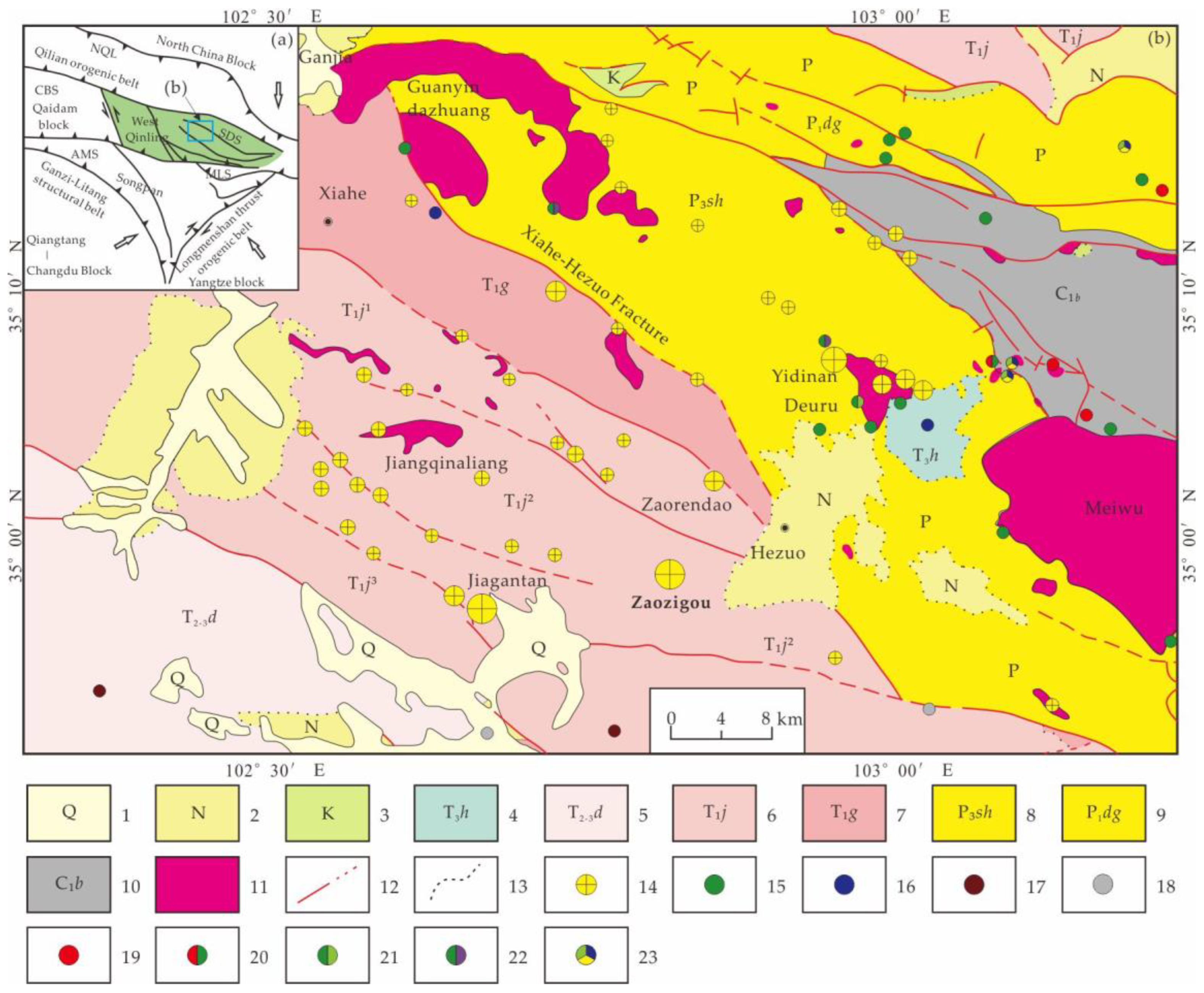
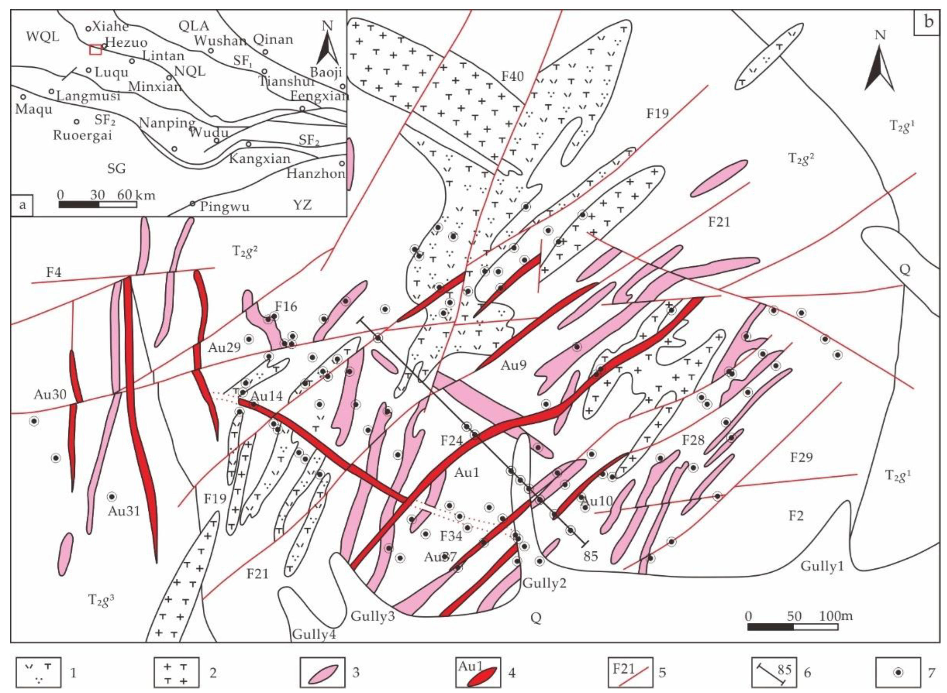
2.1. Geological Setting

The West Qinling is located at the western part of the Qinling orogenic belt, with the Qilian orogenic belt to the north, the Qaidam block to the west, and the songpan block to the south (Figure 1a) [57,58,59,60].

The geotectonic position of the Xiahe-Hezuo area is located at the northwestern part of the West Qinling orogenic belt and at the western extension of the Qinling–Qilian–Kunlun central orogenic belt, whose complex geological structure creates a superior mineralization environment [61].

The Zaozigou Gold deposit is located within the West Qinling fold belt and is a typical epithermal-type gold deposit in the Xiahe-Hezuo area (Figure 1a). The main controlling factors for mineral resources formation within the region are tectonic movement and magmatism [62], with the regional tectonics spreading in a NW direction with developing folds and fracturs. Complex geological structure and magmatism are dominated by Yanshan period intermediate-acid intrusive rocks, which are widely distributed in the form of the batholith, stock, apophysis, and veins [62] (Figure 1b).

Figure 1. (a) Geotectonic location of the study area. NQL: North Qinling tectonic belt; SDS: Shangdan suture zone; CBS: Caibei suture zone; AMS: A’nyemaqen suture zone. (b) Geological map of Xiahe-Hezuo area (modified from [62]). 1. Quaternary; 2. Neogene; 3. Cretaceous;4. Upper Triassic Huari group; 5. Middle-Lower Triassic Daheba group; 6. Lower Triassic Jiangligou group; 7. Lower Triassic Guomugou group; 8. Upper Permian Shiguan group; 9. Lower Permian Daguanshan group; 10. Upper Carboniferous Badu group; 11. Intermediate-acid intrusive rocks; 12. Fracture; 13. Angular unconformity; 14. Gold depsit; 15. Copper deposit; 16. Lead depsit; 17. Antimony deposit; 18. Mercury deposit; 19. Iron deposit; 20. Iron–copper deposit; 21. Copper–molybdenum deposit; 22. Copper-tungsten deposit; 23. Polymetallic deposit.

Figure 1. (a) Geotectonic location of the study area. NQL: North Qinling tectonic belt; SDS: Shangdan suture zone; CBS: Caibei suture zone; AMS: A’nyemaqen suture zone. (b) Geological map of Xiahe-Hezuo area (modified from [62]). 1. Quaternary; 2. Neogene; 3. Cretaceous;4. Upper Triassic Huari group; 5. Middle-Lower Triassic Daheba group; 6. Lower Triassic Jiangligou group; 7. Lower Triassic Guomugou group; 8. Upper Permian Shiguan group; 9. Lower Permian Daguanshan group; 10. Upper Carboniferous Badu group; 11. Intermediate-acid intrusive rocks; 12. Fracture; 13. Angular unconformity; 14. Gold depsit; 15. Copper deposit; 16. Lead depsit; 17. Antimony deposit; 18. Mercury deposit; 19. Iron deposit; 20. Iron–copper deposit; 21. Copper–molybdenum deposit; 22. Copper-tungsten deposit; 23. Polymetallic deposit.

The Triassic strata are the main stratigraphy for gold deposit. The genesis and spatial-temporal evolution of the intermediate-acidic dike is closely related to gold mineralization in the area, and during the mineralization process, the magmatic rocks not only provide the mineralized material, but also their internal environment is very suitable as an ore-bearing space, which can be regarded as a significant mineralization indicator for gold mineralization [63].

The spatial distribution of mineral deposits is directly controlled by the geotectonic position in the Xiahe-Hezuo area, which plays a major role in the formation of different types of gold deposits and is the boundary of the belt from a spatial perspective. The most important types of mineral-controlling structures are fractures and folds in this area [64,65]. The main orebodies of the Zaozigou deposit are produced in NE, NW, and near-SN oriented fracture zones, with two apparent mineralization periods, and post-formation fractures have modified and destroyed the orebodies [66,67,68,69,70].

The Zaozigou gold deposit is a typical representative of gold deposits associated with intermediate-acid dike rocks in the south of the Xiahe-Hezuo fracture. It is located at approximately 9 km southwest of the Hezuo city, Gansu Province, with convenient access to the mine site (Figure 2a). The main ore-bearing position is between Gully 1 and Gully 4, with a total area of approximately 2.6 km² (Figure 2b).

There are only Triassic and Quaternary strata exposed in the Zaozigou gold deposit (Figure 2b). The strata of the area are mainly the lower part of the Gulangdi group (T₂g¹) of the Middle Triassic formation, and the Quaternary (Q_h^alp) is developed in the intermountain valley. The lower part of the Gulangdi group (T₂g¹) is the main ore-bearing rock, which is a set of fine clastic rocks consisting of siliceous slate, clastic feldspathic fine sandstone with interbedded siltstone slate and argillaceous slate. The formation is composed of a large sedimentary cycle from bottom to top consisting of siltstone → argillaceous slate → calcareous slate [66,72].

The fractures are well developed and have a complex morphology, forming an intersecting trend, indicating that the area has experienced multiple phases of geological activity. Fractures strictly control the distribution of orebodies and vein rocks within the deposit. They can be classified into five groups of orientations, namely NW, N-S, NE, E-W, and NNE [73,74]. Fracture structures are the structural surfaces of mineralization, and these structural surfaces control the spreading characteristics of the orebodies [75].

Intermediate-acid dike, including fine crystalline diorite, diorite porphyrite, biotite dioritic porphyrite, and quartz diorite porphyrite densely produced with a porphyritic structure, spreading in NNE direction, turning to a nearly N-S direction in the western part of the deposit and a few NW directions. Influenced by the regional multi-period deep fracture activity, the multi-period magmatism has overlapped on multi-phases mineralization within the deposit [76].

There are 147 gold orebodies have been found in the Zaozigou gold deposit, of which 17 orebodies are main ore bodies with gold reserves greater than 1 tonne, and the total gold reserves of more than 100 tonnes [71]. According to the spatial distribution and combination of the mineralization, Zaozigou deposit can be divided into eastern and western ore groups.

The Eastern ore group is mainly located between Gully 1 and Gully 3 with the strike of NE orientation, containing Au1 controlled by F24, Au9 controlled by F21, and Au15 controlled by F25. These orebodies extend over 1000 m long and 300 m wide, with a NW direction tendency and steep dip near the ground surface, locally nearly upright. In the deep, these orebodies have been staggered by gently dipping fracture, causing the tendency to change to SE orientation (Figure 2b). In addition, orebodies M4 and M6 are laying underground, with the strike of NWW orientation, the tendency of SW orientation, and the dip of 8°~26°. These orebodies cross the NE-striking orebodies obliquely, staggering them, and their own mineralization behavior occurs simultaneously [77].

The Western ore group is mainly distributed between Gully 3 and Gully 4, spreading in a nearly N-S direction, with August 29~August 31 as the main orebodies. The orebodies extend over 1000 m long and wider than 500 m, with a strike of 350°~10°, varying tendency and dips greater than 75°, locally subvertical. These orebodies extend, and the mineralization is weaker in the steeper parts and stronger in the shallower parts.

2.2. Datesets Description

Historical geological and geochemical data were completed, including geological reports, geological exploration maps, and drills geochemical data, from the Development Research Center of China Geological Survey and No.3 Geological and Mineral Exploration team, Gansu Provincial Bureau of Geology and Mineral Exploration and Development, the coordinate system used in the mine-scale is Gaussian Kruger projection coordinates.

This study collected 72 drillings data in the Zaozigou gold deposit, established a drilling location database, an assay database, an inclinometry database, and a lithology database. The 3D model of drillings was constructed based on the drill hole data database (Figure 3).

The primary geochemical halo data from the drillings were collected from the “Zaozigou gold successive resources exploration project in Hezuo city, Gansu Province”, with a total of 72 drillings and 5028 samples with 12 elements of Ag, As, Au, Cu, Hg, Pb, Zn, Sb, W, Bi, Co, and Mo (the element detection methods can refer literature [71]). The sampling method was the continuous picking method with sample intervals generally within 10 m. Some orebodies or strongly altered areas being sampled at decreased intervals.

3. Methodology

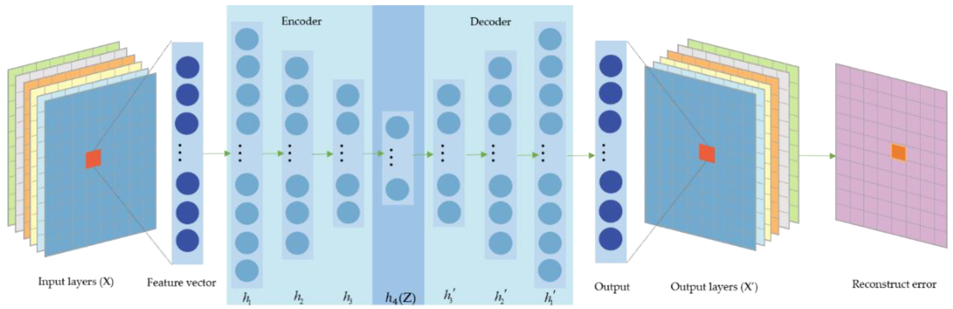
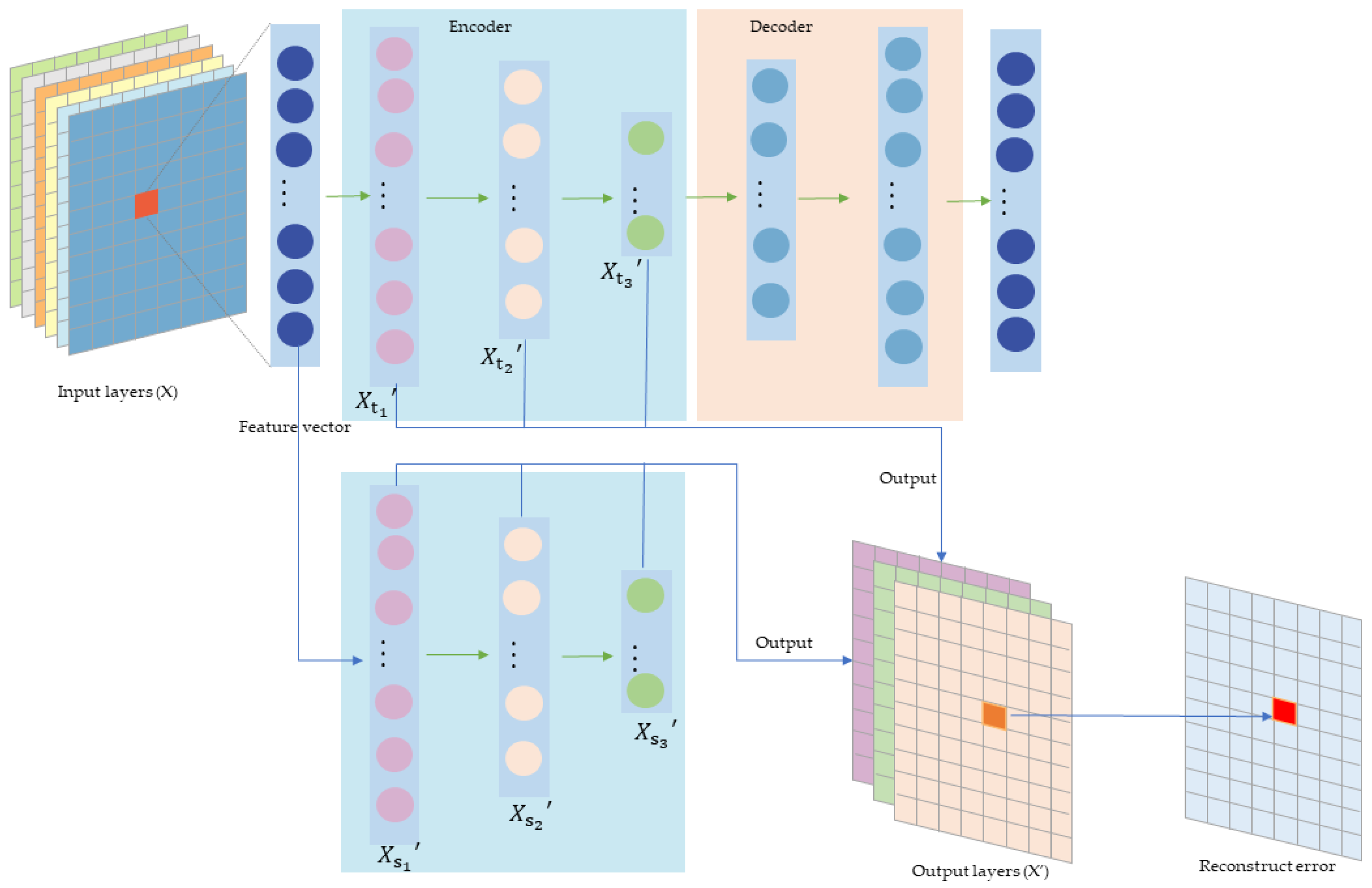
3.1. Deep Auto-Encoder Network

3.1.1. Network Structure Designing

The basic end-to-end structure of DAE and STOAD consists of the input layer (Input), convolutional layer (CONV), activation function layer, and output layer (Output).

DAE is a method that uses neural networks to compress and reconstruct data, and its core is to use an Encoder to compress the original data X to obtain the intermediate variable Z, and then use a Decoder to reconstruct Z to obtain X’ (Figure 4). It can be widely applied to tasks such as data dimensional reduction, feature extraction, and anomaly detection.

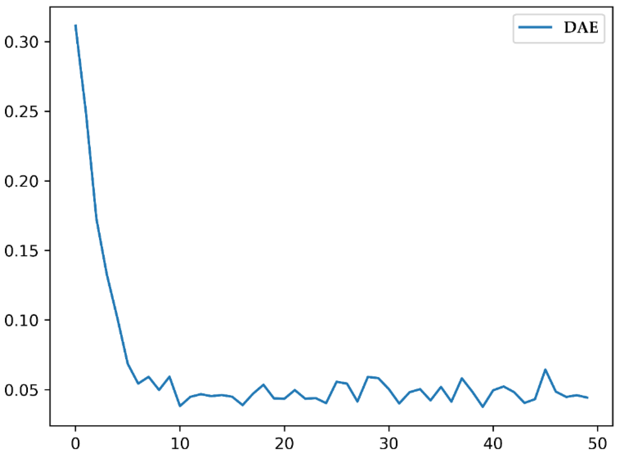
3.1.2. Model Training

In the DAE model, the objective function is to measure the error between the reconstructed sample and the real sample and back propagate to adjust the network parameters. Mean Square Error (MSE) is usually used as the objective function in the reconstruction problem, and the optimization process is mainly divided into three steps: (i) forward propagation for calculating the output, (ii) calculating the loss of reconstruction, and (iii) back propagation to calculating the gradient according to the loss for optimizing the model parameters.

$$x^l=\sigma \left(z^l\right)=\sigma \left(W^l{x}^{l-1}+b^l\right)$$

(1)

Equation (1) express the calculation process from the $l-1$th layer to the $l$th layer of CNN, where $x^l$ represents the features of the $l$th layer (e.g., $x^1$ represents the input data,$x^2$ represents the output obtained after the first layer of convolution and activation calculation), $b^l$ represents the bias term of the $l$th layer, $W^l$ represents the weight parameter of the convolution of the $l$th layer, $Z^l$ represents the intermediate variables of the $l$th layer without the activation function calculation, and $\sigma$ is the activation function. Rectified Linear Unit (ReLU) function is used as the activation function in this paper.

Assuming that the DAE model has a total of $L$ layers, the errors of the input data and the reconstructed data are calculated by MSE to obtain the loss value.

$$Loss=J\left(W,b,x,y\right)=\frac{1}{2}\parallel \sigma \left(z^L\right)-x^1{\parallel }_2^2=\frac{1}{2}\parallel \sigma \left(W^L{x}^{L-1}+b^L\right)-x^1{\parallel }_2^2$$

(2)

${\delta }^L$ is the partial derivatives of Loss to $z^L$,

$${\delta }^L=\frac{\partial J\left(W,b,x,y\right)}{\partial z^L}=\frac{\partial J\left(W,b,x,y\right)}{\partial x^L}\odot {\sigma }^{\prime }\left(z^L\right)$$

(3)

$${\delta }^l=\frac{\partial J\left(W,b,x,y\right)}{\partial z^{l+1}}\frac{\partial z^{l+1}}{\partial z^l}={\left(\frac{\partial z^{l+1}}{\partial z^l}\right)}^T{\delta }^{l+1}={\left(W^{l+1}\right)}^T{\delta }^{l+1}\odot {\sigma }^{\prime }\left(z^l\right)$$

(4)

The partial derivatives of $W$ and $b$ are calculated from the losses, and $\odot$ is the Hadamard product.

$$\frac{\partial J\left(W,b,x,y\right)}{\partial W^l}=\frac{\partial J\left(W,b,x,y\right)}{\partial z^l}\frac{\partial z^l}{\partial w^l}={\delta }^l{\left(x^{l-1}\right)}^T; \frac{\partial J\left(W,b,x,y\right)}{\partial b^l}=\frac{\partial J\left(W,b,x,y\right)}{\partial z^l}\frac{\partial z^l}{\partial b^l}={\delta }^l$$

(5)

The gradient of the back-propagation of each convolutional layer can be calculated by Equation (5), and finally the convolutional kernel parameters are updated by the following two equations. $\alpha$ is the learning rate.

$$W^{l+1}=W^{l+1}-\alpha \frac{\partial J\left(W,b,x,y\right)}{\partial W^{l+1}}$$

(6)

$$b^{l+1}=b^{l+1}-\alpha \frac{\partial J\left(W,b,x,y\right)}{\partial b^{l+1}}$$

(7)

where $l=1,2,3\dots ,L-1$, the above steps are repeated to achieve the training of the DAE network.

3.1.3. Model Testing

In the testing process, the test data X are reconstructed by DAE to obtain X’, MSE between X and X’ is normalized. Setting the threshold value μ, when the MSE value is greater than μ, corresponding samples are judged as anomalies, otherwise, the sample is normal. The calculation equations are as follows.

$$\mathrm{Error}\left(X\right)=\parallel X-X^{\prime }{\parallel }_2^2$$

(8)

$$\mathrm{Predict}\left(X\right)=MinMa{x}_{0-1}\left\{\parallel X-X^{\prime }{\parallel }_2^2\right\}=\{\begin{array}{cc}1,& Predict\left(X\right)\ge \mu \\ 0,& Predict\left(X\right)<\mu \end{array}$$

(9)

3.2. KD-Based STOAD Model

3.2.1. Network Structure Design

KD [78] is a mainstream method applied to model compression, which mainly consists of the Teacher network (T) and Student network (S). The larger T network is usually trained first for the tasks of image classification, target detection, semantic segmentation, etc., and then the smaller S network is trained to learn the generalization ability of the T network. Compared with T-networks, S-networks have fewer parameters and faster computation speed.

Different information will be contained at different depth of the network. For fully extract metallogenic information, the STOAD model is proposed to achieve anomaly detection of layers based on calculating the differences between T encoder and S network. STOAD is divided into two structures: The T network and the S network, where the T network has the same Encoder and Decoder as the DAE, and the S network has the same structure as the Encoder in the T network. Especially, three scales output are designing to express different information at different depth of the network.

In the training process, STOAD model uses all layers to pre-train the T network for reconstruction. The encoder in the T network can be recognized as having the ability to compress the layers, and thus can be seen as having the ability to handle both normal and abnormal data [79]. If the T network is not trained, the anomaly detection can be achieved, but the feature extraction of the T network is not clear, and the interpretability is poor. Sequentially, taking normal data as input, training the S network, calculating the three scale output differences of T encoder and S network using MSE, while h_i, i = 1, 2, 3, are the scales represents different depth of the network. Finally, back-propagates to update the parameters of the S network, the S network only has the capacity of handling normal data learned from the encoder of T network.

In the testing process, taking all data as input. Since the S network only learns the ability of dealing with normal data from the encoder of T network, the S network is difficult to maintain the similar multiscale output features with the T network because of a larger MSE. Therefore, the anomaly detection can be achieved by the MSE values (Figure 5). In contrast to DAE, STOAD not only has three outputs, but also uses multiple levels of semantic and detailed information to make full use of the information in the data for anomaly detection.

3.2.2. Model Training and Testing

The training loss of STOAD consists of two parts, which are the training loss of the T network and the S network

The overall T-network can be considered as a DAE, and MSE is used as the reconstruction loss of the T-network, so that the encoder part of the T-network holds the data compress capability. The training loss of the T network can be calculated as follow equation.

$$Los{s}_{\mathrm{teacher}}=\frac{1}{2}\parallel X-X\prime {\parallel }_2^2$$

(10)

The loss of the S network consists of the MSEs of the three scales output of the T network. In order for the S network to learn the normal data compression ability from the T network, let h₁ = h₂ = h₃ = 1/3, and the training loss of the S network is calculated by Equation (8).

$$Los{s}_{\mathrm{student}}={\displaystyle \sum }_{i=1}^3\frac{1}{2}{h}_i\parallel X_{{\mathrm{t}}_{\mathrm{i}}}-X_{{\mathrm{s}}_{\mathrm{i}}}{\parallel }_2^2$$

(11)

The STOAD model training and testing process is mainly as follows.

• The essence of T-network is a DAE, and its training process is same with DAE referring to Section 3.1.2.
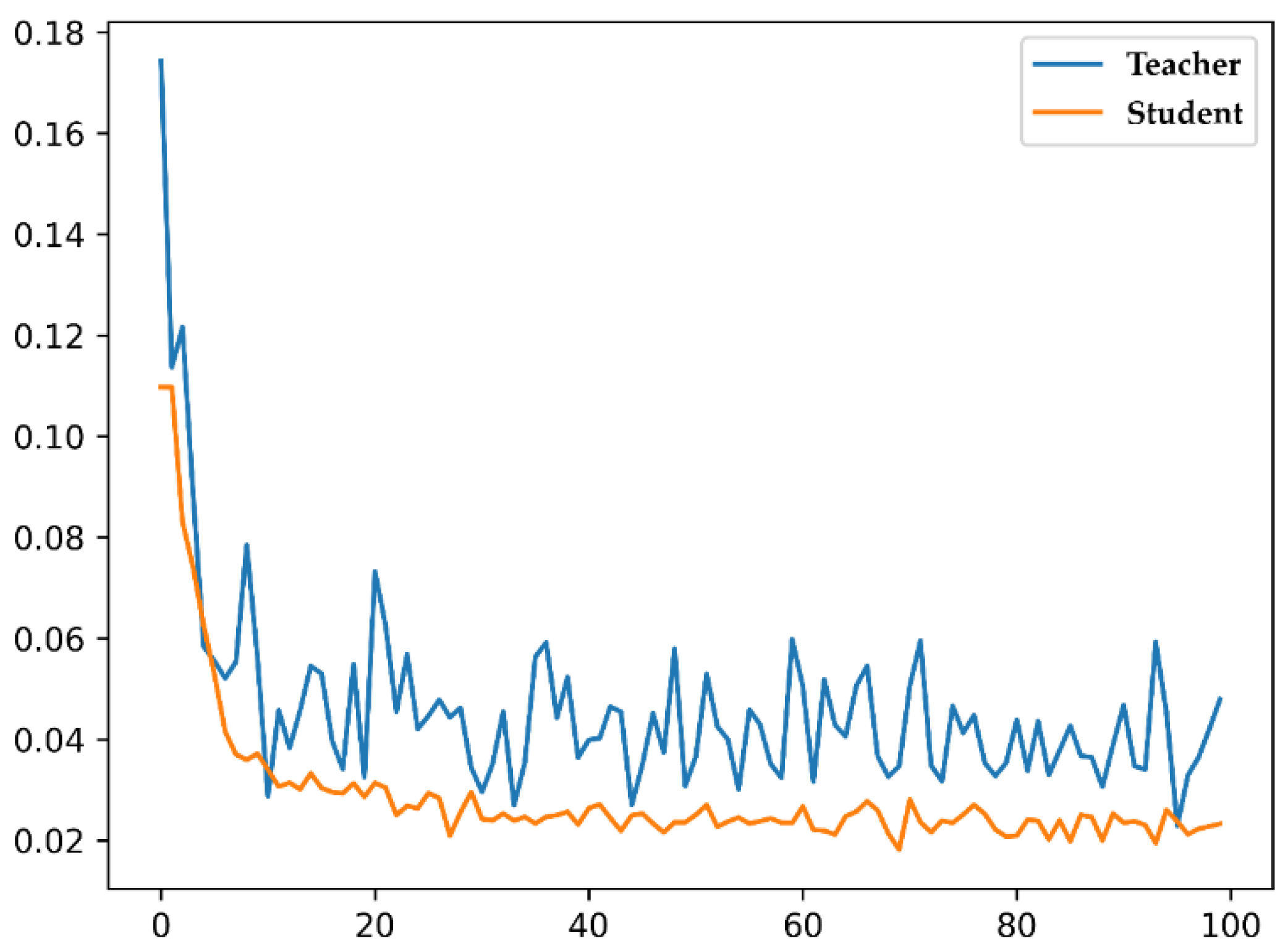
• The S-network update is similar to the T-network, mainly in calculating the loss of the multi-scale features output from the encoder of the T-network, and using only normal data for training, thus letting the S-network to only learn the ability to compress normal data. L is the depth of S network.

  $$Los{s}_{\mathrm{student}}=J\left(W,b,x,y\right)={\displaystyle \sum }_{i=1}^3\frac{1}{2}{h}_i\parallel \sigma \left(W_{\mathrm{t}}{}^{i+1}{x}^i+b_{\mathrm{t}}{}^{i+1}\right)-\sigma \left(W_{\mathrm{s}}{}^{i+1}{x}^i+b_{\mathrm{s}}{}^{i+1}\right){\parallel }_2^2$$

  (12)

${\delta }^L$ is the partial derivatives of $z^L$ of S network.

$${\delta }^L=\frac{\partial J\left(W,b,x,y\right)}{\partial z^L}={\displaystyle \sum }_{i=1}^3\frac{1}{2}{h}_i\frac{\partial J\left(W,b,x,y\right)}{\partial x^L}\odot {\sigma }^{\prime }\left(z^L\right)$$

(13)

and the ${\delta }^l$ is, i is 1 to $L-1$:

$${\delta }^l=\frac{\partial J\left(W,b,x,y\right)}{\partial z^{l+1}}\frac{\partial z^{l+1}}{\partial z^l}={\left(\frac{\partial z^{l+1}}{\partial z^l}\right)}^T{\delta }^{l+1}={\left(W^{l+1}\right)}^T\odot {\sigma }^{\prime }\left(z^l\right){\delta }^{l+1}$$

(14)

$$\frac{\partial J\left(W,b,x,y\right)}{\partial W^l}=\frac{\partial J\left(W,b,x,y\right)}{\partial z^l}\frac{\partial z^l}{\partial w^l}={\delta }^l{\left(x^{l-1}\right)}^T$$

(15)

$$\frac{\partial J\left(W,b,x,y\right)}{\partial b^l}=\frac{\partial J\left(W,b,x,y\right)}{\partial z^l}\frac{\partial z^l}{\partial b^l}={\delta }^l$$

(16)

Convolutional module is updated by the following two equations. $\alpha$ is the learning rate.

$$W^{l+1}=W^{l+1}-\alpha \frac{\partial J\left(W,b,x,y\right)}{\partial W^{l+1}}$$

(17)

$$b^{l+1}=b^{l+1}-\alpha \frac{\partial J\left(W,b,x,y\right)}{\partial b^{l+1}}$$

(18)

where $l=1,2,\dots ,L-1$.

In the testing process, we used T and S networks to calculate the testing dataset, separately. Defining the weights of three scales are $W_{h1}=W_{h2}=W_{h3}=1/3$, the weighted sum of the output can be calculated by Equation (19), where $X_{{\mathrm{t}}_{\mathrm{i}}}$ and $X_{{\mathrm{s}}_{\mathrm{i}}}$ represent the output of the Encoder part of the T network and the S network, respectively. Predict (x) is the normalized Error (x), selecting a threshold μ, when the Predict (x) is greater than μ the sample point is judged to be an abnormal sample, otherwise it is a normal sample.

$$\mathrm{Error}\left(x\right)={\displaystyle \sum }_{i=1}^3{h}_i\parallel X_{{\mathrm{t}}_i}-X_{{\mathrm{s}}_i}{\parallel }_2^2$$

(19)

$$\mathrm{Predict}\left(x\right)=MinMa{x}_{0-1}\{{\displaystyle \sum }_{i=1}^3{h}_i\parallel X_{{\mathrm{t}}_i}-X_{{\mathrm{s}}_i}{\parallel }_2^2\}=\{\begin{array}{cc}1,& Predict\left(x\right)\ge \mu \\ 0,& Predict\left(x\right)<\mu \end{array}$$

(20)

4. Results

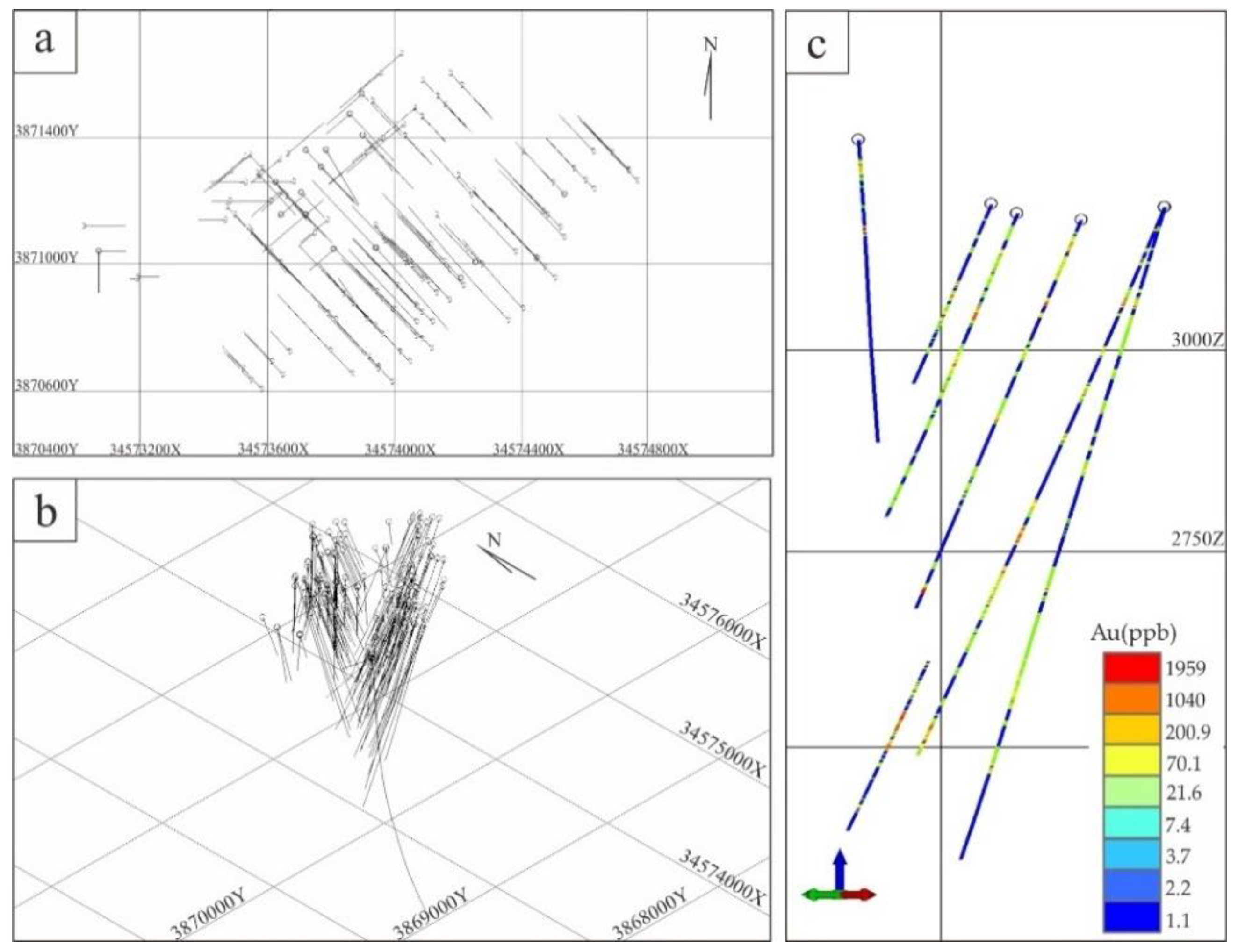
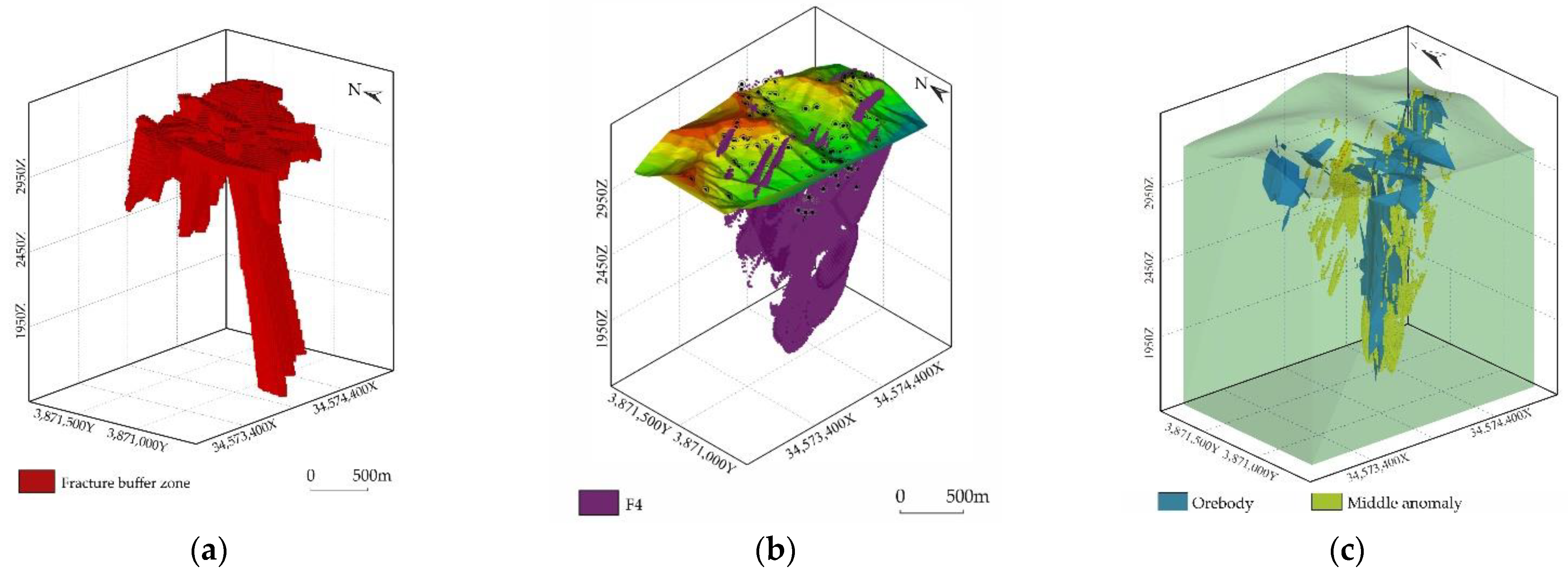
4.1. Geological and Geochemical Quantitative Prediction Model at Depth of Zaozigou Gold Deposit

Before carrying out the deep quantitative mineral prospectivity mapping in the Zaozigou gold deposit, it is necessary to review the geological and geochemical quantitative prediction model established in previous work [80].

Orebodies are strictly controlled by fractures in the Zaozigou gold deposit. The 30 m buffer zone of the fractures can effectively reflect the influence range of fracture, which can be used as a mineral prediction indicator. Factor F4 is an element association of Sb-Hg, which has a close relationship with fractures, and can be used as a favorable indicator for inferring deep fractures. The middle anomaly area of Au extracted by the multiple fractal C-V model can well reflect the spatial distribution of orebodies, which should be used as an important quantitative indicator. Near-ore halo element association B2 is extracted by the knowledge-driven CoDA also can express the location of orebodies well, it should be another mineral prediction indicator. The ratio of front halo to tail halo is an important geochemical parameter for predicting orebodies, B1/B3 is regarded as a prediction indicator accordingly (

Table 1. Geological and geochemical quantitative mineral resource prediction model at depth of the Zaozigou gold deposit.

Ore-Forming Factor	Description	Prediction Indicator	Variables
Geology	fracture	Influence range of fracture	30 m buffer zone
		Element association of fracture	Hg-Sb (F4)
Geochemistry	Ore-forming element	Geochemical anomaly	Au
	Primary geochemical halo	Element association of near-ore halo	Au-Ag-Cu-Pb-Zn (B2)
		Geochemical parameter (Front halo/tail halo)	As-Sb-Hg (B1)/W-Bi-Co-Mo (B3)

; Figure 6). The detailed data analysis and interpretation can refer to the literature [80].

4.2. Training Sample Selection

For mineralization prediction, the target variable (i.e., the label of training samples) is either mineralized or nonmineralized (denoted by 1 and 0, respectively). A total of 39,306 positive samples extracted from known orebodies and 49,686 negative samples extracted from the nonmineralized position confirmed by drillings are used as training dataset. In contrast to mineralization generates concentrated in limited space, the non-mineralization is a widespread phenomenon, and negative samples are selected to be distributed as randomly and uniformly as possible throughout the study area [81] (Figure 7).

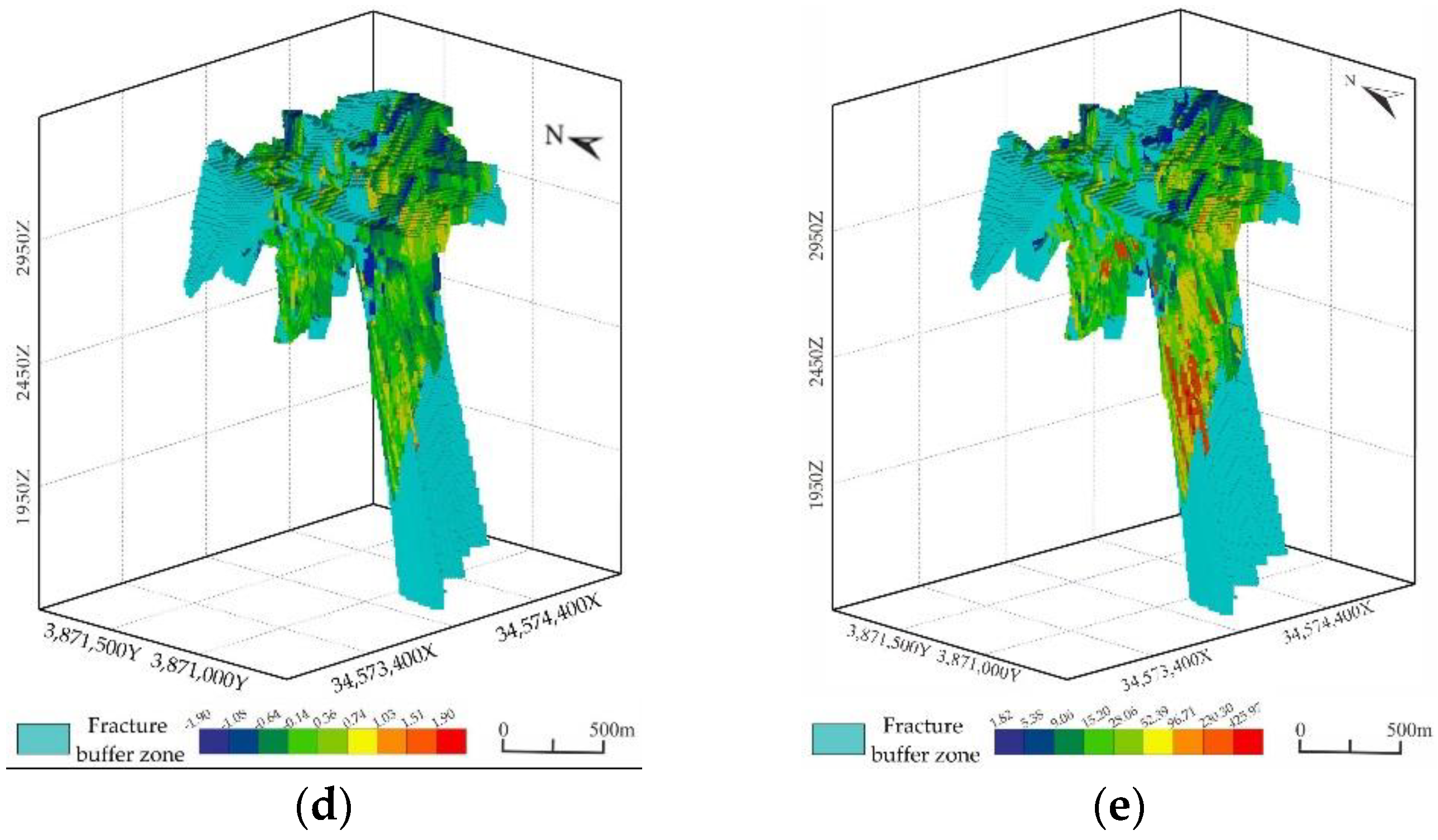
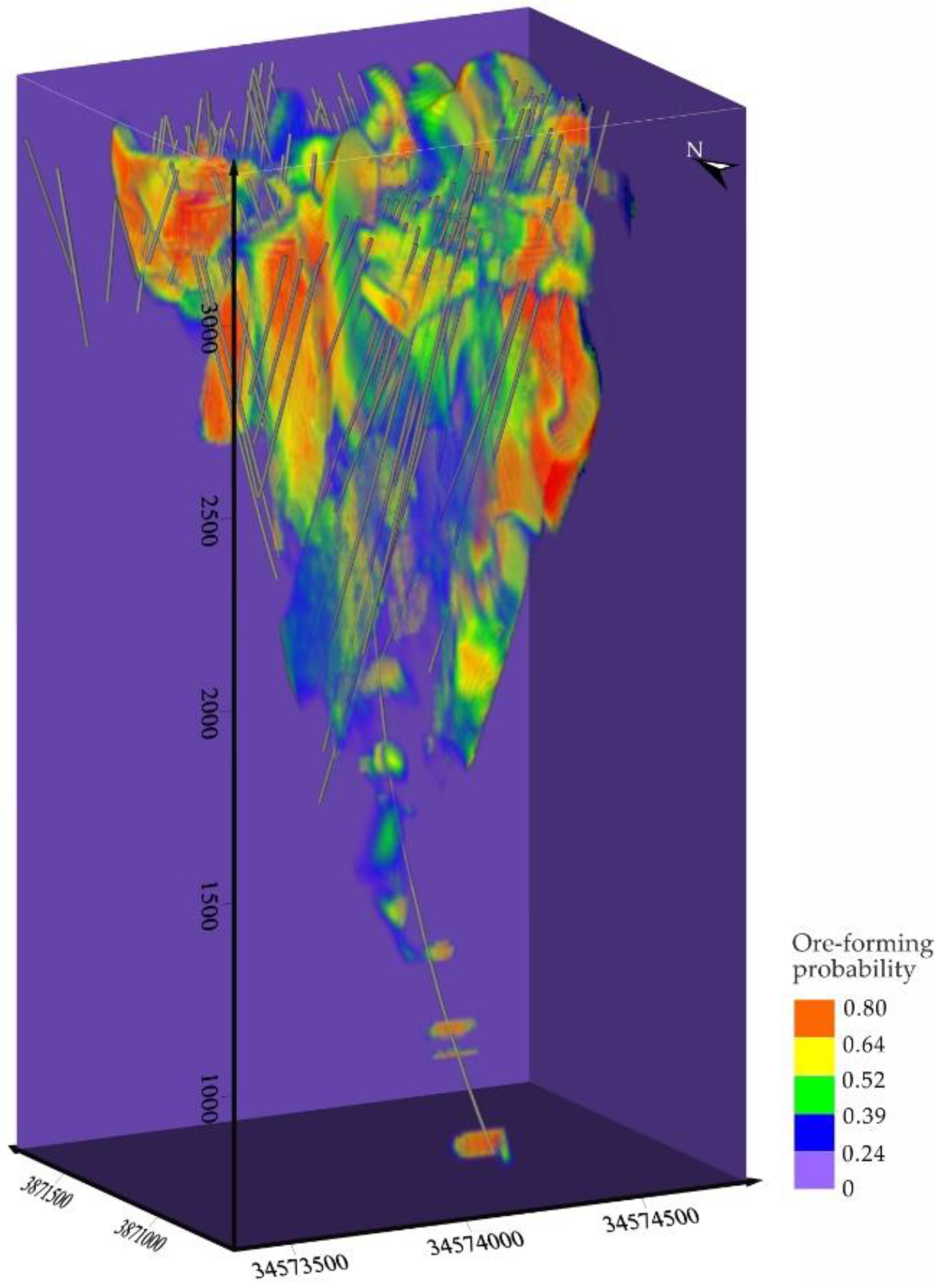
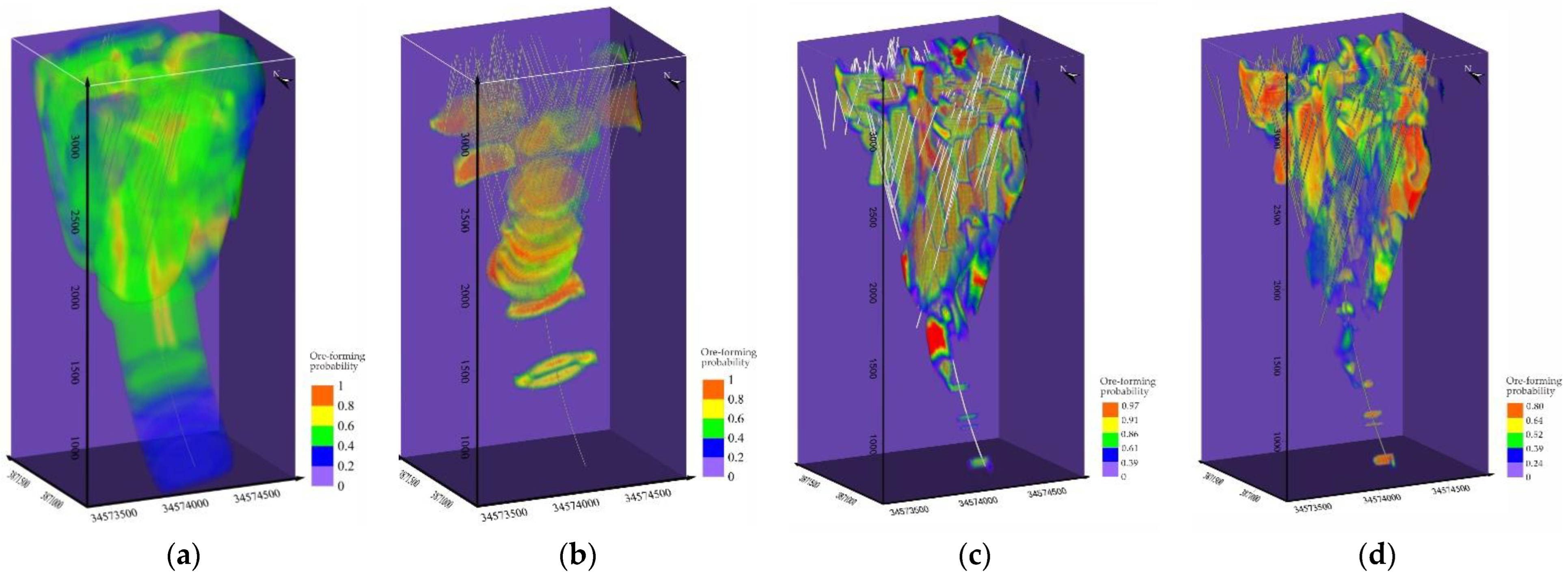
4.3. DAE-Based 3D MPM

DAE is a widely used unsupervised model in deep learning. In this study, the DAE model is constructed by convolution, and the training process automatically learns to extract the semantic features of the normal evidence layer to compress and reconstruct the corresponding layers. In the testing process, detecting ore-induced anomalies by MSE value, the higher the MSE value is, the greater the loss of reconstruction is, which illustrates the high-probability area of ore-forming.

This DAE model is built using python 3.8, PyTorch 1.71 framework, the optimizer is Adam, the batch size is 16, the learning rate is 0.001, the learning rate decay is 10% per 5 Epochs, the CPU is 12th Gen Intel(R) Core(TM) i7-127OOKF, and the GPU is NVIDIA GeForce RTX 3090.

DAE model uses 70% of the normal data for training, and the testing dataset includes the remaining 30% of the normal samples and the relatively small number of anomaly samples. The DAE model is trained for 500 Epochs and the loss function is plotted as follows. The model relatively converges at an MSE value of about 0.025, but the MSE fluctuates wider (Figure 8). In Figure 4 and Figure 6, the horizontal axis indicates the sampling order and the vertical axis indicates the loss of DAE. The prediction parameters of precision value reaches 93%, Recall value is 88%, and F1-measure is 90%, which demonstrate the high accuracy and reliability of DAE-based MPM. It clearly shows that the high ore-forming probability at depth of Zaozigou gold deposit, which is worth for further investigation (Figure 9).

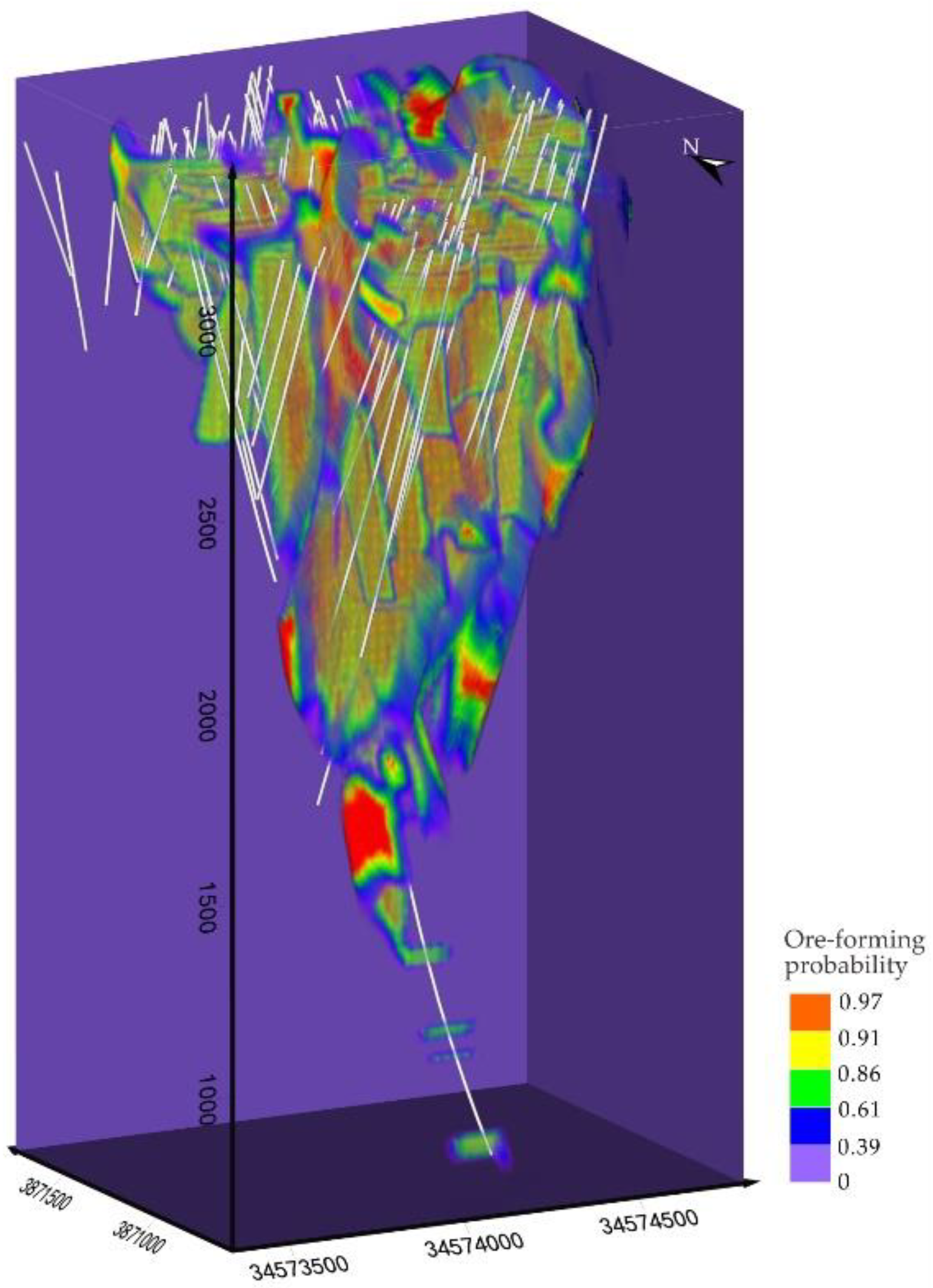
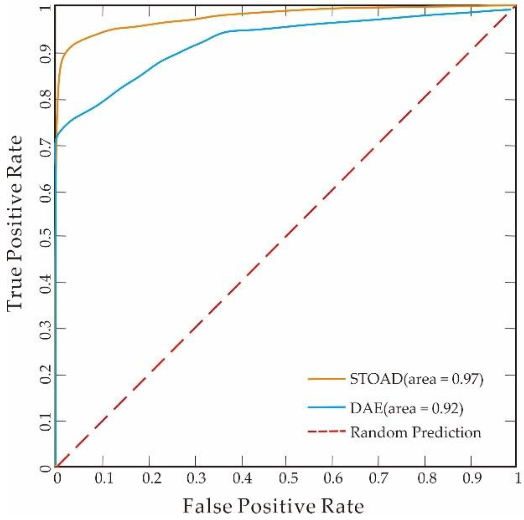
4.4. STOAD-Based 3D Mineral Prospectivity Mapping

The STOAD model is implemented using python 3.8, and PyTorch 1.71 framework. The T network is mainly composed of two parts: encoder and Decoder. The structure of T network is symmetric for letting the number of parameters of both parts identical, and thus the data compression ability of encoder is approximately equal to the data reconstruction ability of Decoder.

The S network only has the encoder part, which is consistent with the T encoder. ReLU activation function is used for its capability of dealing with nonlinear data.

The same training parameters are used in the T and S networks, with an optimizer of Adam, a batch size of 16, a learning rate of 0.001, and a learning rate decay of 10% per 5 Epochs.

Similarly, STOAD uses 70% of the normal data for training, and the testing dataset includes the remaining 30% of the normal samples and the relatively small number of anomaly samples.

The STOAD model is trained with 500 Epochs, and the Teacher loss function and the Student loss function are plotted in Figure 10, the T network converges at about MSE value of 0.025 (similar to the above DAE), and fluctuates wider. The MSE curve of the S network converges at a lower value of about 0.0125, and distributes more stable than T network. The loss of the T network is the same as DAE indicating the ability to reconstruct all training data, the loss of the S network represents the difference in output between the S and T networks, and the more stable loss of the S network means that the S network can learn better the ability of the T network to reconstruct normal data.

The prediction parameter of Precision value reaches 96%, Recall value is 90%, and F1 value is 93%.

The 3D MPM based on STOAD model shows the high ore-forming probability at depth of Zaozigou gold deposit which has the similar characteristics ore-forming probability distribution at depth. It gives evidence for deep mineral resources prediction (Figure 11).

5. Discussion

In this study, the deep learning methods of DAE and STOAD model are carried out for 3D MPM in Zaozigou gold deposit.

Compared with the DAE model, STOAD model has a higher precision in detection of ore-induced anomalies, which demonstrates a higher reliability of 3D MPM (Figure 9 and Figure 11).

Meanwhile, the ROCs of the two methods were used to evaluate the models, and the AUC values of the two methods were 0.92 of DAE and 0.97 of STOAD. Observably, the STOAD model expresses a higher performance (Figure 12).

From the points of algorithm theory, the STOAD model is proposed based on the KD idea combined with the DAE network, which is an improvement of DAE. So, it is better than the conventional DAE model in terms of algorithm performance.

From the points of application, the results of quantitative mineral resources prediction show that STOAD is more accurate and robust, which is demonstrated by prediction parameters, the loss curve (Figure 8 and Figure 10) and the ROC curve (Figure 12).

Furthermore, a total of 4 methods, two machine learning methods (MaxEnt model and GMM) and two deep learning methods (DAE and STOAD model), have been carried out for 3D MPM (Figure 13). The machine learning-based 3D MPM can refer to the literature [80], which is the previous work of our research team.

The prediction results of the four methods exhibit a high correlation with the known orebodies in the shallow part and a slight difference in the deep part (Figure 13). From the comparative analysis of the prediction results and model performance among the four methods, the STOAD takes advantage of mathematical theory and has the highest AUC value (Figure 14). Especially, the high probability area can better reflect the metallogenic regularity at large depth. Therefore, it is decided to delineate a comprehensive mineral exploration targets at large depth of the Zaozigou based on the prediction results of STOAD model and supported by the prediction results of other methods. In order to improve the prediction accuracy, the area with a logical probability greater than 0.75 and less than 0.998 is defined as a medium potential area, and the area with a logical probability greater than 0.998 is defined as a high potential area, based on which three main mineral exploration targets are circled (Figure 15).

Target I is located at elevation 1600~2000 m, belongs to the NE-orientation orebody group, which should be the extension of the Au1 orebody. In this position, we developed the main ore-forming fracture. The Au and Sb concentration in this position, and the ratio of front halo to tail halo has been increasing. Especially, it appears high logical probability calculated by all four methods at this position, indicating the Au1 orebody may extends deeper than the elevation of 1800 m or a concealed orebody exist therein.

Target II is located in the NW-orientation orebody group at the elevation of 2000~2400 m, where the fractures distribute complex, and the tail halo element Co has a significant vertical overlap with the front halo elements Sb and As. The elevated geochemical parameters starting from 2600 m to deep indicate that there may be an extension of ore bodies or new blind orebodies at depth. According to the theory of primary halo zonation, the front halo indicators generally appear at the leading edge of the ore body 100–300 m, and the blind ore body will appear at an altitude of 2400 m deep.

Target III is located below 1600 m, it can be divided into targets III-1, III-2, and III-3. Target III-1 is located at elevation of about 1300 m, target III-2 located at elevation of about 1000 m., target III-3 located at elevation of 700 m. The deep fracture is the main indicator. It is worth mentioning that the deep drill for scientific research has achieved in 2021, which is the deepest drill of Zaozigou gold deposit, which reaches to the elevation of 700 m (Figure 15). In previous study, there may be an “upper veins and lower layers” distribution feature of orebodies [82]. The shallow stratigraphy is strongly folded, and steeply dipping fracture structures are developed; the orebody is controlled by fractures and vein rocks, while the deep orebody may be mainly controlled by intrusive mass to form laminated ore bodies. This understanding is also reflected in the present prediction targets.

6. Conclusions

To address the scientific problem of quantitative mineralization prediction at large depth, the geological and geochemical quantitative mineral resources prediction model at depth of the Zaozigou gold deposit is constructed based on the quantitative extraction of mineralization signatures, which consists of five quantitative prediction indicators, including 30 m fracture buffer zone, element association (Sb-Hg) of ore-bearing structures, metallogenic element Au, near-ore halo element association Au-Ag-Cu-Pb-Zn, and the ratio of front halo to tail halo (As-Sb-Hg)/(W-Mo-Bi). Then, two machine learning methods (MaxEnt model and GMM) and two deep learning methods (DAE and STOAD model) are carried out for 3D MPM, and mineral exploration targets are delineated at depth (Figure 15).

Because the primary halo of drills is limited by the engineering-controlled boundaries, this study adopts the idea of quantitative expression of ore-controlling factors by element associations and limit the deep inference range within the modeling space to perform deep quantitative mineral prediction. However, the accuracy of the prediction of machine learning and deep learning methods inevitably decreases rapidly with increasing depth. This shortcoming can be supplemented by two aspects of quantitative inversion of geophysical data and numerical simulation of deep mineralization dynamics, which is also a direction worth further research.

In summary, a series of methods are developed in this study of 3D Mineral Prospectivity Mapping of Zaozigou gold deposit, West Qinling, China. The achieved results by machine learning and deep learning methods shows well performance in quantitative mineral resources prediction at depth, which is worth being promoted to similar ore deposits. Moreover, it was concluded that the deep learning-based approach works better with larger amounts of data, and the STOAD proposed in this paper has a higher accuracy in anomaly detection. May the relevant ideas of this study provide a reference for related researchers.

References

1. Frits, A. Principles of probabilistic regional mineral resource estimation. Earth Sci. 2011, 36, 189–200. [Google Scholar]
2. Zhou, Y.Z.; Zuo, R.G.; Liu, G.; Yuan, F.; Mao, X.C.; Guo, Y.J.; Xiao, F.; Liao, J.; Liu, Y.P. The Great-leap-forward Development of Mathematical Geoscience During 2010–2019: Big Data and Artificial Intelligence Algorithm Are Changing Mathematical Geoscience. Bull. Mineral. Petrol. Geochem. 2021, 40, 556–573. [Google Scholar]
3. Liu, Z.; Li, L.; Fang, X.; Qi, W.; Shen, J.; Zhou, H.; Zhang, Y. Hard-rock tunnel lithology prediction with TBM construction big data using a global-attention-mechanism-based LSTM network. Automation in Construction. 2021, 125, 103647. [Google Scholar] [CrossRef]
4. Cheng, Q.M. What are Mathematical Geosciences and its frontiers? Earth Sci. Front. 2021, 28, 6–25. [Google Scholar]
5. Zuo, R.G. Deep Learning-Based Mining and Integration of Deep-Level Mineralization Information. Bull. Mineral. Petrol. Geochem. 2019, 38, 53–60. [Google Scholar]
6. Zuo, R.G.; Peng, Y.; Li, T.; Xiong, Y.H. Challenges of Geological Prospecting Big Data Mining and Integration Using Deep Learning Algorithms. Earth Sci. 2021, 46, 350–358. [Google Scholar]
7. Zhang, Q.; Zhou, Y.Z. Big data will lead to a profound revolution in the field of geological science. Chin. J. Geol. 2017, 52, 637–648. [Google Scholar]
8. Zhou, Y.Z.; Li, P.X.; Wang, S.G.; Xiao, F.; Li, J.Z.; Gao, L. Research progress on big data and intelligent modelling of mineral deposits. Bull. Mineral. Petrol. Geochem. 2017, 36, 327–331. [Google Scholar]
9. Zhou, Y.Z.; Wang, J.; Zuo, R.G.; Xiao, F.; Shen, W.J.; Wang, S.G. Machine learning, deep learning and Python language in field of geology. Acta Petrol. Sin. 2018, 34, 3173–3178. [Google Scholar]
10. Sun, S.; He, Y.X. Multi-label emotion classification for microblog based on CNN feature space. Adv. Eng. Sci. 2017, 49, 162–169. [Google Scholar]
11. Simonyan, K.; Zisserman, A. Very deep convolutional networks for large-scale image recognition. arXiv 2014, arXiv:1409.1556. [Google Scholar]
12. Martens, J.; Sutskever, I. Learning recurrent neural networks with hessian-free optimization. In Proceedings of the 28th International Conference on International Conference on Machine Learning, Bellevue, WD, USA, 28 June 2011–2 July 2011. [Google Scholar]
13. Bengio, Y.; Lamblin, P.; Popovici, D.; Larochelle, H. Greedy layer-wise training of deep networks. Adv. Neural Inf. Process. Syst. 2006, 19, 153–160. [Google Scholar]
14. Sainath, T.N.; Kingsbury, B.; Ramabhadran, B. Auto-encoder bottleneck features using deep belief networks. In Proceedings of the 2012 IEEE International Conference on Acoustics, Speech and Signal Processing (ICASSP), Kyoto, Japan, 25–30 March 2012; pp. 4153–4156. [Google Scholar]
15. Hinton, G. Deep Belief Nets. In Encyclopedia of Machine Learning; Sammut, C., Webb, G.I., Eds.; Springer: Boston, MA, USA, 2011; pp. 267–269. [Google Scholar] [CrossRef]
16. Ciresan, D.; Giusti, A.; Gambardella, L.; Schmidhuber, J. Deep neural networks segment neuronal membranes in electron microscopy images. Adv. Neural Inf. Process. Syst. 2012, 25, 2843–2851. [Google Scholar]
17. Lin, N. Study on the Metallogenic Prediction Models Based on Remote Sensing Geology and Geochemical Information: A Case Study of Lalingzaohuo Region in Qinghai Province; Jilin University: Changchun, China, 2015. [Google Scholar]
18. Yan, G.; Xue, Q.; Xiao, K.; Chen, J.; Miao, J.; Yu, H. An analysis of major problems in geological survey big data. Geol. Bull. China 2015, 34, 1273–1279. [Google Scholar]
19. Holtzman, B.K.; Paté, A.; Paisley, J.; Waldhauser, F.; Repetto, D. Machine learning reveals cyclic changes in seismic source spectra in Geysers geothermal field. Sci. Adv. 2018, 4, o2929. [Google Scholar] [CrossRef] [Green Version]
20. Rouet Leduc, B.; Hulbert, C.; Lubbers, N.; Barros, K.; Humphreys, C.J.; Johnson, P.A. Machine learning predicts laboratory earthquakes. Geophys. Res. Lett. 2017, 44, 9276–9282. [Google Scholar] [CrossRef]
21. Zhou, Y.Z.; Chen, S.; Zhang, Q.; Xiao, F.; Wang, S.G.; Liu, Y.P.; Jiao, S.T. Advances and prospects of big data and mathematical geoscience. Acta Petrol. Sin. 2018, 34, 255–263. [Google Scholar]
22. Zuo, R.; Xiong, Y. Big data analytics of identifying geochemical anomalies supported by machine learning methods. Nat. Resour. Res. 2018, 27, 5–13. [Google Scholar] [CrossRef]
23. Xiong, Y.; Zuo, R.; Carranza, E.J.M. Mapping mineral prospectivity through big data analytics and a deep learning algorithm. Ore Geol. Rev. 2018, 102, 811–817. [Google Scholar] [CrossRef]
24. Zhong, Z.; Sun, A.Y.; Yang, Q.; Ouyang, Q. A deep learning approach to anomaly detection in geological carbon sequestration sites using pressure measurements. J. Hydrol. 2019, 573, 885–894. [Google Scholar] [CrossRef] [Green Version]
25. Zuo, R.G. Exploration geochemical data mining and weak geochemical anomalies identification. Earth Sci. Front. 2019, 26, 67. [Google Scholar]
26. Li, C.; Jiang, Y.L.; Hu, M.K. Study and application of gravity anomaly separation by cellular neural networks. Comput. Tech. Geophys. Geochem. Explor. 2015, 37, 16–21. [Google Scholar]
27. Cai, H.H.; Zhu, W.; Li, Z.X.; Liu, Y.Y.; Li, L.B.; Liu, C. Prediction method of Tungsten-molybdenum prospecting target area based on deep learning. J. Geo-Inf. Sci. 2019, 21, 928–936. [Google Scholar]
28. Li, S.; Chen, J.; Xiang, J. Applications of deep convolutional neural networks in prospecting prediction based on two-dimensional geological big data. Neural Comput. Appl. 2020, 32, 2037–2053. [Google Scholar] [CrossRef]
29. Li, T.; Zuo, R.; Xiong, Y.; Peng, Y. Random-drop data augmentation of deep convolutional neural network for mineral prospectivity mapping. Nat. Resour. Res. 2021, 30, 27–38. [Google Scholar] [CrossRef]
30. Zuo, R. Geodata science-based mineral prospectivity mapping: A review. Nat. Resour. Res. 2020, 29, 3415–3424. [Google Scholar] [CrossRef]
31. Zuo, R.; Wang, Z. Effects of random negative training samples on mineral prospectivity mapping. Nat. Resour. Res. 2020, 29, 3443–3455. [Google Scholar] [CrossRef]
32. Ran, X.; Xue, L.; Zhang, Y.; Liu, Z.; Sang, X.; He, J. Rock classification from field image patches analyzed using a deep convolutional neural network. Mathematics 2019, 7, 755. [Google Scholar] [CrossRef] [Green Version]
33. Sang, X.; Xue, L.; Ran, X.; Li, X.; Liu, J.; Liu, Z. Intelligent high-resolution geological mapping based on SLIC-CNN. ISPRS Int. J. Geo-Inf. 2020, 9, 99. [Google Scholar] [CrossRef] [Green Version]
34. Guo, J.; Li, Y.; Jessell, M.W.; Giraud, J.; Li, C.; Wu, L.; Li, F.; Liu, S. 3D geological structure inversion from Noddy-generated magnetic data using deep learning methods. Comput. Geosci.-UK 2021, 149, 104701. [Google Scholar] [CrossRef]
35. Rezaei, A.; Hassani, H.; Moarefvand, P.; Golmohammadi, A. Determination of unstable tectonic zones in C–North deposit, Sangan, NE Iran using GPR method: Importance of structural geology. J. Min. Environ. 2019, 10, 177–195. [Google Scholar]
36. Rezaei, A.; Hassani, H.; Moarefvand, P.; Golmohammadi, A. Lithological mapping in Sangan region in Northeast Iran using ASTER satellite data and image processing methods. Geol. Ecol. Landsc. 2020, 4, 59–70. [Google Scholar] [CrossRef] [Green Version]
37. Liu, Y.P.; Zhu, L.X.; Zhou, Y.Z. Application of Convolutional Neural Network in prospecting prediction of ore deposits: Taking the Zhaojikou Pb-Zn ore deposit in Anhui Province as a case. Acta Petrol. Sin. 2018, 34, 3217–3224. [Google Scholar]
38. Liu, Y.P.; Zhu, L.X.; Zhou, Y.Z. Experimental Research on Big Data Mining and Intelligent Prediction of Prospecting Target Area—Application of Convolutional Neural Network Model. Geotecton. Metallog. 2020, 44, 192–202. [Google Scholar]
39. Cai, H.H.; Xu, Y.Y.; Li, Z.X.; Cao, H.H.; Feng, Y.X.; Chen, S.Q.; Li, Y.S. division of metallogenic prospective areas based on convolutional neural network model: A case study of the Daqiao gold polymetallic deposit. Geol. Bull. China 2019, 38, 1999–2009. [Google Scholar]
40. Li, S.; Chen, J.; Liu, C.; Wang, Y. Mineral prospectivity prediction via convolutional neural networks based on geological big data. J. Earth Sci.-China 2021, 32, 327–347. [Google Scholar] [CrossRef]
41. Sun, T.; Li, H.; Wu, K.; Chen, F.; Zhu, Z.; Hu, Z. Data-driven predictive modelling of mineral prospectivity using machine learning and deep learning methods: A case study from southern Jiangxi Province, China. Minerals 2020, 10, 102. [Google Scholar] [CrossRef] [Green Version]
42. Zhang, S.H. Deep Learning for Mineral Prospectivity Mapping of Lala-Type Copper Deposit in the Huili Region, Sichuan; China University of Geoscience: Beijing, China, 2020. [Google Scholar]
43. Yang, N.; Zhang, Z.; Yang, J.; Hong, Z.; Shi, J. A convolutional neural network of GoogLeNet applied in mineral prospectivity prediction based on multi-source geoinformation. Nat. Resour. Res. 2021, 30, 3905–3923. [Google Scholar] [CrossRef]
44. Zhang, S.; Carranza, E.J.M.; Wei, H.; Xiao, K.; Yang, F.; Xiang, J.; Zhang, S.; Xu, Y. Data-driven mineral prospectivity mapping by joint application of unsupervised convolutional auto-encoder network and supervised convolutional neural network. Nat. Resour. Res. 2021, 30, 1011–1031. [Google Scholar] [CrossRef]
45. Rumelhart, D.E.; Hinton, G.E.; Williams, R.J. Learning representations by back-propagating errors. Nature 1986, 323, 533–536. [Google Scholar] [CrossRef]
46. Wang, Y.; Yao, H.; Zhao, S. Auto-encoder based dimensionality reduction. Neurocomputing 2016, 184, 232–242. [Google Scholar] [CrossRef]
47. Hinton, G.E.; Salakhutdinov, R.R. Reducing the dimensionality of data with neural networks. Science 2006, 313, 504–507. [Google Scholar] [CrossRef] [PubMed] [Green Version]
48. Hou, B.; Kou, H.; Jiao, L. Classification of polarimetric SAR images using multilayer autoencoders and superpixels. IEEE J.-Stars. 2016, 9, 3072–3081. [Google Scholar] [CrossRef]
49. Lv, F.; Han, M.; Qiu, T. Remote sensing image classification based on ensemble extreme learning machine with stacked autoencoder. IEEE Access 2017, 5, 9021–9031. [Google Scholar] [CrossRef]
50. Nayak, R.; Pati, U.C.; Das, S.K. A comprehensive review on deep learning-based methods for video anomaly detection. Image Vis. Comput. 2021, 106, 104078. [Google Scholar] [CrossRef]
51. Kingma, D.P.; Welling, M. Auto-encoding variational bayes. arXiv 2013, arXiv:1312.6114. [Google Scholar]
52. Zhang, S.; Xiao, K.; Carranza, E.J.M.; Yang, F.; Zhao, Z. Integration of auto-encoder network with density-based spatial clustering for geochemical anomaly detection for mineral exploration. Comput. Geosci.-UK 2019, 130, 43–56. [Google Scholar] [CrossRef]
53. Xiong, Y.; Zuo, R.; Luo, Z.; Wang, X. A physically constrained variational autoencoder for geochemical pattern recognition. Math. Geosci. 2022, 54, 783–806. [Google Scholar] [CrossRef]
54. Luo, Z.; Zuo, R.; Xiong, Y.; Wang, X. Detection of geochemical anomalies related to mineralization using the GANomaly network. Appl. Geochem. 2021, 131, 105043. [Google Scholar] [CrossRef]
55. Li, Q.; Jin, S.; Yan, J. Mimicking very efficient network for object detection. In Proceedings of the IEEE Conference on Computer Vision and Pattern Recognition, Honolulu, HI, USA, 21–26 July 2017; pp. 6356–6364. [Google Scholar]
56. Tung, F.; Mori, G. Similarity-preserving knowledge distillation. In Proceedings of the IEEE/CVF International Conference on Computer Vision, Seoul, Korea; 2019; pp. 1365–1374. [Google Scholar]
57. Feng, Y.M.; Cao, X.Z.; Zhang, E.P.; Hu, Y.X.; Pan, X.P.; Yang, J.L.; Jia, Q.Z.; Li, W.M. Tectonic Evolution Framework and Nature of The West Qinling Orogenic Belt. Northwest. Geol. (Xi’an, China) 2003, 36, 1–10, (In Chinese with English Abstract). [Google Scholar]
58. Wei, L.X. Tectonic Evolution and Mineralization of Zaozigou Gold Deposit, Gansu Province. Master’s Thesis, China University of Geosciences, Beijing, China, 2015. (In Chinese with English Abstract). [Google Scholar]
59. Zeng, J.J.; Li, K.N.; Yan, K.; Wei, L.L.; Huo, X.D.; Zhang, J.P. Tectonic Setting and Provenance characteristics of the Lower Triassic Jiangligou Formation in West Qinling-Constraints from Geochemistry of Clastic Rock and zircon U-Pb Geochronology of Detrital Zircon. Geol. Rev. 2021, 67, 1–15, (In Chinese with English Abstract). [Google Scholar]
60. Li, Z.B.; Liu, Z.Y.; Li, R. Geochemical Characteristics and metallogenic Potential Analysis of Daheba Formation in Ta-Ga Area of Gansu Province. Contrib. Geol. Miner. Resour. Res. 2021, 36, 187–194, (In Chinese with English Abstract). [Google Scholar]
61. Chen, Y.; Wang, K.J. Geological Features and Ore Prospecting Indicators of Sishangou Silver Deposit. Gansu. Metal. 2015, 37, 108–111, (In Chinese with English Abstract). [Google Scholar]
62. Di, P.F. Geochemistry and Ore-Forming Mechanism on Zaozigou gold deposit in Xiahe-Hezuo, West Qinling, China. Ph.D. Thesis, Lanzhou University, Lanzhou, China, 2018. (In Chinese with English Abstract). [Google Scholar]
63. Li, K.N.; Li, H.R.; Liu, B.C.; Yan, K.; Jia, R.Y.; Wei, L.L. Geochemical characteristics of TTG Dick rock and the Relation with Gold Mineralization in West Qinling Mountain. Sci. Tech. Engrg. 2019, 19, 52–65, (In Chinese with English Abstract). [Google Scholar]
64. Kang, S.S. Geological Characteristics and Prospecting Criteria of Nanmougou Copper Deposit, Gansu Province. Gansu. Metal. 2018, 40, 79–85, (In Chinese with English Abstract). [Google Scholar]
65. Kang, S.S.; Dou, X.G.; Zhi, C.; Wu, X.L. Geochemical Characteristics and Genetic Analysis of the Namugou Copper Deposit in Sunan County, Gansu. Gansu. Metal. 2019, 41, 65–72, (In Chinese with English Abstract). [Google Scholar]
66. Liu, Y. Relationship between Intermediate-acid Dike Rock and Gold Mineralization of the Zaozigou Deposit, Gansu Province. Master’s Thesis, Chang’an University, Xi’an, China, 2013. (In Chinese with English Abstract). [Google Scholar]
67. Hu, J.Q. Mineral Control Factors, Metallogenic Law and Prospecting Direction of Integrated Gold Mine Exploration Area in Shilijba-Yangshan Area of Gansu Province. Gansu. Sci. Technol. 2018, 34, 27–33. (In Chinese) [Google Scholar]
68. Zhao, J.Z.; Chen, G.Z.; Liang, Z.L.; Zhao, J.C. Ore-body Geochemical Features of Zaozigou Gold Deposit. Gansu. Geol. 2013, 22, 38–43, (In Chinese with English Abstract). [Google Scholar]
69. Lu, J. Study on Characteristics and Ore-host Regularity of Gold Mineral in the Western Qinling Region, Gansu Province. Master’s Thesis, China University of Geosciences, Beijing, China, 2016. (In Chinese with English Abstract). [Google Scholar]
70. Zhang, Y.N.; Liang, Z.L.; Qiu, K.F.; Ma, S.H.; Wang, J.L. Overview on the Metallogenesis of Zaozigou gold deposit in the West Qinling Orogen. Miner. Explor. 2020, 11, 28–39, (In Chinese with English Abstract). [Google Scholar]
71. Tang, L.; Lin, C.G.; Cheng, Z.Z.; Jia, R.Y.; Li, H.R.; Li, K.N. 3D Characteristics of Primary Halo and Deep Prospecting Prediction in The Zaozigou Gold Deposit, Hezuo City, Gansu Province. Geol. Bull. China 2020, 39, 1173–1181, (In Chinese with English Abstract). [Google Scholar]
72. Chen, G.Z.; Wang, J.L.; Liang, Z.L.; Li, P.B.; Ma, H.S.; Zhang, Y.N. Analysis of Geological Structures in Zaozigou Gold Deposit of Gansu Province. Gansu. Geol. 2013, 22, 50–57, (In Chinese with English Abstract). [Google Scholar]
73. Chen, G.Z.; Liang, M.L.; Wang, J.L.; Zhang, Y.N.; Li, P.B. Characteristics and Deep Prediction of Primary Superimposed Halos in The Zaozigou Gold Deposit of Hezuo, Gansu Province. Geophys. Geochem. Explor. 2014, 38, 268–277, (In Chinese with English Abstract). [Google Scholar]
74. Jin, D.G.; Liu, B.C.; Chen, Y.Y.; Liang, Z.L. Spatial Distribution of Gold Bodies in Zaozigou Mine of Gansu Province. Gansu. Geol. 2015, 24, 25–30+41, (In Chinese with English Abstract). [Google Scholar]
75. Zhu, F.; Wang, G.W. Study on Grade Model of Gansu Zaozigou Gold Mine Based on Geological Statistics. Acta Mineral. Sin. 2015, 35, 1065–1066. (In Chinese) [Google Scholar]
76. Chen, G.Z.; Li, L.N.; Zhang, Y.N.; Ma, H.S.; Liang, Z.L.; Wu, X.M. Characteristics of fluid inclusions and deposit formation in Zaozigou gold mine. J. Jilin Univ. (Earth Sci. Ed.) 2015, 45, 1–2. (In Chinese) [Google Scholar]
77. Wu, X.M. Study on Geological Characteristics and Metallogenic Regularity of the Gelouang Gold Deposit. Master’s Thesis, Lanzhou University, Lanzhou, China, 2018. (In Chinese with English Abstract). [Google Scholar]
78. Hinton, G.; Vinyals, O.; Dean, J. Distilling the knowledge in a neural network. arXiv 2015, arXiv:1503.02531. [Google Scholar]
79. Wang, G.; Han, S.; Ding, E.; Huang, D. Student-teacher feature pyramid matching for unsupervised anomaly detection. arXiv 2021, arXiv:2103.04257. [Google Scholar]
80. Yunhui, K.; Guodong, C.; Bingli, L.; Miao, X.; Zhengbo, Y.; Cheng, L.; Yixiao, W.; Yaxin, G.; Shuai, Z.; Hanyuan, Z.; et al. 3D Mineral Prospectivity Mapping of Zaozigou gold deposit, West Qinling, China: Machine Learning-based mineral prediction. Minerals 2022, in press.
81. Carranza, E.J.M. Geochemical Anomaly and Mineral Prospectivity Mapping in GIS; Elsevier: Amsterdam, The Netherlands, 2008. [Google Scholar]
82. Development Research Center of China Geological Survey. The report of mineral resources potential assessment and mineral resources prediction at depth in the Maqu-Hezuo area, Gansu province. 2021; (Unpublished Work). [Google Scholar]
Figure 2. (a) Regional location of study area. QLA = Qilian tectonic belt; WQL: West Qinling tectonic belt; NQL: North Qaidam tectonic belt; SF1: Wushan–Tianshui–Shangdan suture zone; SF2: Maqu-Nanping–Lueyang suture zone; SG: Songpan–Ganzi tectonic belt; YZ: Yangtze block. (b) Geological map of Zaozigou gold deposit (modified from [71]). 1. Quartz diorite porphyrite; 2. Granodiorite-porphyry; 3. Plagioclase granite porphyry; 4. Gold orebody; 5. Fracture; 6. Mineral exploration line; 7. Drilling Hole.
Minerals 12 01382 g002
Figure 3. 3D model of Drillings in Zaozigou gold deposit. (a) Plan view of drillings distribution. (b) Side view of drillings distribution. (c) Sample grade distribution of drillings.
Minerals 12 01382 g003
Figure 4. Network structure of DAE.
Minerals 12 01382 g004
Figure 5. STOAD network structure.
Minerals 12 01382 g005
Figure 6. (a) Fracture buffer zone; (b) Element association of fracture; (c) Au anomaly; (d) Element association of near-ore halo; (e) Geochemical parameter (Front halo/tail halo).
Minerals 12 01382 g006aMinerals 12 01382 g006b
Figure 7. Distribution of positive samples and negative samples.
Minerals 12 01382 g007
Figure 8. The training loss of DAE model.
Minerals 12 01382 g008
Figure 9. DAE-based 3D MPM.
Minerals 12 01382 g009
Figure 10. The training loss of STOAD model.
Minerals 12 01382 g010
Figure 11. STOAD-based 3D MPM.
Minerals 12 01382 g011
Figure 12. ROC curves of the DAE and STOAD.
Minerals 12 01382 g012
Figure 13. Comparison of the 3D MPM of 4 methods. (a) MaxEnt mode. (b) GMM. (c) DAE model. (d) STOAD model.
Minerals 12 01382 g013
Figure 14. ROC curves of 4 methods, MaxEnt model, GMM, DAE model and STOAD model.
Minerals 12 01382 g014
Figure 15. Comprehensive mineral exploration targets.
Minerals 12 01382 g015