Geometallurgical Characterisation with Portable FTIR: Application to Sediment-Hosted Cu-Co Ores

Abstract

Cobalt (Co) mine production primarily originates from the sediment-hosted copper (Cu) deposits of the Democratic Republic of Congo (DRC). These deposits usually consist of three ore zones with a supergene oxide ore blanket overlying a transition zone which grades into a sulphide zone at depth. Each of these zones display a mineral assemblage with varying gangue mineralogy and, most importantly, a distinct state of oxidation of the mineralisation. This has direct implications for Cu and Co extraction during mineral processing as it dictates which processing method is to be used (i.e., leaching vs. flotation) and affects the performance of these. To optimise resource efficiency, reduce technical risks and environmental impacts, comprehensive understanding of variation of ore mineralogy and texture in the deposit is essential. By defining geometallurgical ore types according to their inferred metallurgical behaviour, this information can serve to classify the resources and improve resource management. To obtain insight into the spatial distribution of mineral grades, it is necessary to develop techniques that have the potential to measure rapidly and, preferably, within the mine at relatively low-cost. In this study, the application of portable Fourier transformed infrared (FTIR) spectroscopy is investigated to measure the mineralogy of drill core samples. A set of samples from a sediment-hosted Cu-Co deposit in DRC was selected to test this approach. Results were validated using automated mineralogy (QEMSCAN). Prediction of gangue and target mineral grades from the FTIR spectra was achieved through partial least squares regression (PLS-R) combined with competitive adaptive reweighted sampling (CARS). It is shown that the modal mineralogy obtained from FTIR can be used to classify the ore according to type of mineralisation and gangue mineralogy into geometallurgical ore types. This classification supports selection of a suitable processing route and is likely to affect the overall process performance.

1. Introduction

Geometallurgy is a cross-discipline that seeks to maximise the economic value and improve the sustainability of the extraction of metals and minerals by documenting variability of key geological, mineralogical, and metallurgical ore properties and quantifying their impact on mineral processing and metallurgical processes performance [1,2,3]. The quantitative spatially-based database generated can be readily integrated into a 3D predictive model for mine planning and mineral processing to support production management and reduce technical risks, securing the economical optimisation of the whole operation [3,4,5,6]. Two different approaches exist to link key ore properties to metallurgical process performance, the traditional geometallurgical approach and the particle-based approach. The traditional approach relies on geometallurgical testing of a selection of a large number of geo-referenced test samples to determine metallurgical parameters [4,7,8,9] while the particle-based approach relies on minerals and particles as common parameters for process modelling and simulation [10,11]. Ore mineralogical properties (modal mineralogy, textures, etc.) are the main, if not the most important, geometallurgical ore properties as they define not only the value of the deposit but also the method of extraction and concentration.

This is particularly true for the stratiform sediment-hosted copper-cobalt deposits of the Democratic Republic of Congo (DRC) from which most of the current cobalt mine production originates [12,13]. These deposits usually consist of three main zones: an oxide supergene ore blanket overlying a transitional mixed sulphide-oxide zone grading into a sulphide ore at depth [14,15]. The mineralisation is hosted in a variety of rocks associated with carbonates (mostly dolomite) and carbon-rich lithologies, and siliceous gangue minerals such as quartz and talc. The minerals of economic interest range from oxide minerals such as malachite for copper and heterogenite for cobalt in the supergene zone to sulphide minerals at depth, including carrollite for cobalt, and chalcopyrite and bornite for copper [16,17,18].

1.1. Importance of Ore Mineralogy

The overall mineralogy of the ore, oxidation state of the mineralisation, and gangue composition vary from one zone to the other. This plays a critical role during mineral processing. Indeed, while the oxide ore is usually processed through a leaching/solvent extraction/electrowinning (L/SX/EW) route, the mixed and sulphide ores are usually treated using flotation, sulfating roasting, leaching and electrowinning [12,13]. Gangue mineralogy is considered as the single most important parameter affecting operating costs and recoveries of hydrometallurgical projects [19] and it can be the decisive factor for selection of the processing route [20]. In practice, dolomitic ores are generally harder [15] and the presence of dolomite affects the floatability of oxide copper-cobalt minerals and requires the use of the sulphidisation method [20,21,22] or reverse flotation [23]. Significantly, dolomite is a major sulphuric acid consumer and it often determines whether the ore can be treated economically with sulphuric acid leaching [24]. Other problematic gangue minerals are chlorites which must be removed prior to flotation in order to achieve grades acceptable for further processing of the concentrates [25] and which are also known to be powerful long-term acid consumers [19]. Hence, quantifying both gangue and valuable minerals in the ore is of paramount interest. Moreover, mineral grades are an important input parameter for the mineral-based geometallurgical approach and corresponding process models [26]. To obtain high-resolution insights into the spatial distribution of the ore modal mineralogy, i.e., mineral grades, it is necessary to develop innovative technologies and approaches that have the potential to measure mineral grades within the mine rapidly and, preferably, at low cost.

While modal mineralogy has traditionally been determined by optical microscopy using point counting, there is a trend towards the use of automated techniques, which are both less time-consuming and more accurate. These include quantitative X-ray diffraction (QXRD) with Rietveld refinement [27], optical microscopy image analysis and multispectral imaging [28] and automated mineralogy. Image analysis techniques which interpret scanning electron microscopy (SEM) data (QEMSCAN, MLA, MinSCAN, TESCAN, etc.) provide more rapid quantitative analysis of mineral grades and textures [29,30,31,32,33]. However, within geometallurgical programs, it is desirable to have an ore characterisation technique that is fast, inexpensive and above all practical [34]. The aforementioned techniques are costly, with a turnaround time (including sample preparation) in the range of a few hours and require an experienced operator. More recently, the element-to-mineral conversion (EMC) method, based on the simultaneously solving of a set of mass balance equations formulated between chemical elements and minerals, allows to estimate mineral grades [11]. The method is however, restricted to relatively simple mineralogy with a limited number of minerals not larger than the number of analysed components (major elements, metals). Hence, it is of interest to investigate the use of a hand-held device that can provide a rapid estimate of the modal mineralogy of core samples.

1.2. Infrared Technology

Infrared (IR) is a well-known technology used for mineral identification. Indeed, the IR part of the electromagnetic spectrum can be used to determine the presence of certain minerals by identifying features in a transmitted or reflected spectrum [35,36,37,38]. In particular, near infrared (NIR), as well as hyperspectral visible to near-infrared (VNIR), have been considered as potential tools for ore sorting [39,40,41,42]. The absorption spectra observed in the short-wave infrared (SWIR) region (1300–2400 nm) are due to overtones and combinations of the fundamentals occurring at longer wavelengths [36]. These longer wavelengths (2.5–25 μm), in the mid- and long-wave infrared (MWIR/LWIR) range, host features of intense fundamental molecular vibrations related to chemical components [43]. The intensity of these vibration bands is so high that a mirror-like opacity is induced, leading to high reflectance peaks that are referred to as the reststrahlen band [44]. Silicates, carbonates and hydroxides minerals are known to be active in the MWIR range and display a unique reflectance feature due to fundamental stretching and vibrational motions [45,46].

When interpreting the spectra measured from hard rock or core samples, consisting of complex mineral assemblages, all of which potentially influence the spectrum, overlaps can occur between the characteristic features of individual minerals. Indeed, most of these features are observed at similar wavelengths and this may cause issues with identification of the minerals. When analysing a mixture of minerals, MWIR spectra express a linear combination of the spectra of constituent pure minerals spectra as long as particles are larger than the wavelengths [47]. Authors have suggested that spectral mixing remains essentially linear for particle sizes down to 60 μm and that, with appropriate particle diameter end-member spectra for the corresponding mixtures, the errors are reduced significantly, and linearity continues through to the 10–20 μm size fraction [48]. For smaller particle sizes, however, the volume scattering will influence the spectra, meaning that non-calculated peaks and troughs can appear [44]. Particulate materials may have relatively rough surfaces which cause multiple surface scattering, resulting in a cavity effect that reduces the contrast of the reststrahlen bands. On the other hand, spectra of solid rocks with a relatively smooth surface are dominated by surface scattering, which results in reststrahlen bands with high spectral contrast [49].

Fourier transformed infrared (FTIR) is a rapid, non-destructive, and low-cost method which requires little or no preparation of the sample. FTIR is considered to be one of the most underused tools in applied geology [50]. When obtaining FTIR reflectance spectra, more accurate and complete spectra are measured due to the presence of an interferometer [51]. Quantitative mineralogy of reservoir rocks obtained through both XRD and FTIR showed good agreement between the two techniques [52,53,54] and, in one case, reservoir properties could be directly deduced from FTIR data [55]. FTIR was demonstrated to be a reliable technique to obtain the mineralogy of sediments when applying a generalised least squares inversion against a library of mineral standards with unique IR spectra [56]. Recent developments have shown that application of a bench-scale FTIR equipped with an attenuated total reflection (ATR) sample analysis unit allowed to perform mineral quantification on powdered samples for a wide range of rock matrix (pegmatites, sedimentary rocks) through univariate or multivariate (partial least squares regression) spectral data analysis with satisfactory validation results when compared to XRD [57]. In all previously mentioned studies, a significant amount of sample preparation was performed, as samples were crushed and pelletized before measuring the reflectance spectra. However, only a limited number of studies have attempted to use portable FTIR spectroscopy for quantitative mineralogy from spectra measured directly on drill core sample [58]. While the results obtained in the aforementioned study were promising, the semi-automated method yielded variable accuracy, only allowing for first approximations of mineral distributions.

This paper investigates the development of a practical way to determine modal mineralogy from drill cores of a DRC Cu-Co sediment-hosted ore using portable FTIR technology, with the results being validated by the QEMSCAN analysis. The objective is to develop a simple and robust method that can be used for geometallurgical characterisation or core samples and in-pit ore analyses. The mineralogical information is then used to propose a mineral-based geometallurgical ore-type classification scheme which provides information for subsequent processing steps or pre-concentration strategies depending on the mineralogy of the feed ore.

2. Materials and Methods

2.1. Material

Samples used in this work originate from an operational open pit mine located in the DRC which extracts ore from a sediment-hosted Cu-Co deposit. The operation is currently only processing ore from the oxide horizon through a traditional L/SX/EW process. The process produces cathode copper while cobalt is recovered as a by-product in the form of cobalt hydroxide. We selected 34 quarter core samples representing the variation of cobalt grade, mineralogy and textures within the orebody from a core sample library. The selected samples were cut to produce thin sections for QEMSCAN analysis while the mirror image of these thin sections, which remained on the drill cores, were analysed using handheld FTIR (Figure 1). As a first approximation, this mirrored sample is considered to have the same mineralogical content as the corresponding thin section.

2.2. Fourier Transformed Infrared (FTIR) Spectroscopy

2.2.1. FTIR Measurements

The reflectance spectra were obtained using an Agilent 4300 Handheld FTIR (Edinburgh, UK) with a wavelength range set between 2.5 μm and 15.8 μm, a resolution of 4 cm⁻¹ and a spot size of approximately 5–7 mm. The instrument is fully portable—it is hand-held, weighs less than 2.2 kg and is battery powered. To accommodate potential uneven surfaces that causes light to be reflected at all angles, a diffuse reflectance sample interface was used. This enables measurement of both internal and external reflectance, making it more suitable for reflection from rough surfaces such as those of cut drill cores used in this study [59]. Calibration was performed using a gold/silver standard and 126 background measurements were performed in order to subtract the background noise. Each reflectance spectrum is the average of 64 reflectance measurements, automatically computed by the device. The data from the hand-held device is collected using MicroLab Mobile software (Agilent, Santa Clara, CA, USA). For predictive purposes, all spectra were recorded as the logarithm of the reciprocal reflectance, log(1/R).

For each selected drill core, between 10 and 15 individual measurements were made on the thin section mirrored image using the handled FTIR docked in a stand and moving manually the sample following the workflow described in Figure 2. The individual spectra were averaged to provide an average spectrum for the whole mirrored image which could be compared to the modal mineralogy of the corresponding thin section, as obtained by QEMSCAN. Alternatively, to capture the characteristic features of some key minerals in the ore, fieldscan images from the QEMSCAN analysis were divided into tiles which followed the scheme used for the individual FTIR measurements on the mirrored image. This offers the possibility to compare the tiles modal mineralogy given by the QEMSCAN to the corresponding individual FTIR spectra (Figure 2).

2.2.2. Spectra Pre-Processing

Spectral pre-processing is applied to the raw FTIR data to remove noise and physical phenomena in the spectra in order to improve the subsequent multivariate regression (Figure 3). The pre-processing procedure is performed by a smoothing step using a moving average on a finite-size spectral window, the size of which is optimised for each mineral. Next, two scatter-corrective methods are applied independently, i.e., standard normal variate (SNV) transformation and multiple scatter correction (MSC). Both techniques are very similar and aim to remove the multiplicative interferences of light scattering and particle size. Furthermore, shifts in the baseline of the reflectance spectra transformation were corrected by row centring and row scaling, filtering out multiplicative interferences of scatter and particle size [60]. Data correction is performed using the following equation:

$$x_{corr}=\frac{x_{raw}-b_0{}_{ }}{b_1}$$

(1)

where x_raw is the raw sample spectra measured by the handled FTIR, x_corr is the corrected spectra, and b₀ and b₁ are scalar parameters which differ for each sample. For SNV, b₀ is the average value and b₁ the standard deviation of the sample spectrum to be corrected [61], while for MSC b₀ and b₁ are obtained by least-squares regression fit against a reference spectrum [61]:

$$x_{\mathit{raw}}=b_0+b_1·x_{\mathit{ref}}+\epsilon$$

(2)

where x_ref is a reference spectrum, in this case the average spectrum of the whole sample set and ε is the modelling error. Spectral derivatives were also applied to explore the effect of both additive and multiplicative effects in the spectra and to correct baseline effects in spectra. The 1st derivative of the spectrum is computed using the Savitzky and Golay (SG) algorithm which includes a smoothing step [62]. Details about the SG derivative computation method can be found in the papers [60,62].

2.3. QEMSCAN

Quantitative mineralogical analysis was carried out using a QEMSCAN 4300 at Camborne School of Mines, University of Exeter, UK. This consists of a Zeiss EVO 50 SEM and four light element Bruker silicon drift detector (SDD) X-ray detectors [29,63]. The acquired EDX spectra are combined into one signal and compared to a computer-based database to allow rapid determination of the spatial distribution of the minerals present [64]. Selected samples were prepared into polished uncovered thin sections with a volume of about 100 µm (thickness) × 25 mm (width) × 47 mm (length) and carbon coated to 25 nm prior to analysis using an Emitech K950 carbon coater. The measurement was performed using the following settings: default beam settings of 25 kV and 5 nA, X-ray count rate of 1000 per pixel, a working distance of around 22 mm under high vacuum, and beam calibration every 30 min. To allow for mounting of the sample, a surface area of approximately 20 mm × 38 mm was analysed using the fieldscan measurement mode at an X-ray resolution or pixel spacing of 10 μm and a 1500 μm² field size (×43 magnification). This produced approximately 6 million data points per sample and X-ray signals, and the BSE signal when required, at each point were analysed following standard in-house practice. This included adding and improving SIP (species identification protocol) entries in the database as was deemed appropriate. Development of the database included all copper and cobalt minerals specific to these samples, as reported in Tijsseling et al. (2019). During this process, all mineral categories were checked by examination of elemental abundance, elemental ratios, and BSE signal. All data acquisition was undertaken using the iMeasure v4.2SR1 software and spectral interpretation and data processing used iDiscover software v4.2SR1 and 4.3 [65].

2.4. Multivariate Regression Methods

Partial least squares regression (PLS-R) is generally considered as the most accurate of the available mathematical methods for quantitative evaluation of IR spectra [66]. The main advantages of PLS-R are that it can account for overlapping peaks, sample impurities, and non-linearities in Beer’s Law due to molecular interactions [53]. PLS-R allows modelling of the correlation between a set of predictor variables in the form of a multivariate X matrix (in this case the reflectance data given by the FTIR analysis) and a set of dependent response variables in the form of a Y matrix (in this case the mineral grades as given by the QEMSCAN analysis) by regression. PLS-R models can be interpreted as inter-related principal component analysis (PCA) scores of the predictors, t, and the responses, u, aiming to maximise the covariance between t and u [67]. Like PCA, PLS-R reduces the dimensionality of the predictor matrix by extracting latent variables (LVs) which are linear combinations of all X-variables (PLS components). LVs are correlated to the responses while simultaneously capturing the largest possible amount of variation in the predictors. A detailed description of the PLS-R method and analytical features can be found in the literature [66,67,68,69].

Full spectra, which include all measured wavelengths, contain much redundant information, uninformative data, or noise that often leads to bad prediction results. Hence, it is common practice to select informative wavelengths prior to the establishment of the final regression model. There are many selection techniques but a recently developed method called competitive adaptive reweighted sampling (CARS) has proved to be very efficient when applied to NIR data [70,71,72]. The CARS algorithm chooses an optimal subset of wavelengths, i.e., points in the X-matrix (instrumental data), to build a PLS-R model with the lowest value of root mean square error of cross validation (RMSECV) by selecting the variables with the largest absolute regression coefficients. For a detailed description of the CARS method, refer to Li et al. [70]. The procedure followed for each y (mineral) can be summarised as follows:

I.

A first PLS-R is applied to the full spectrum. The absolute values of regression coefficients of the obtained PLS model are calculated and used as an index for evaluating the importance of each variable.

II.

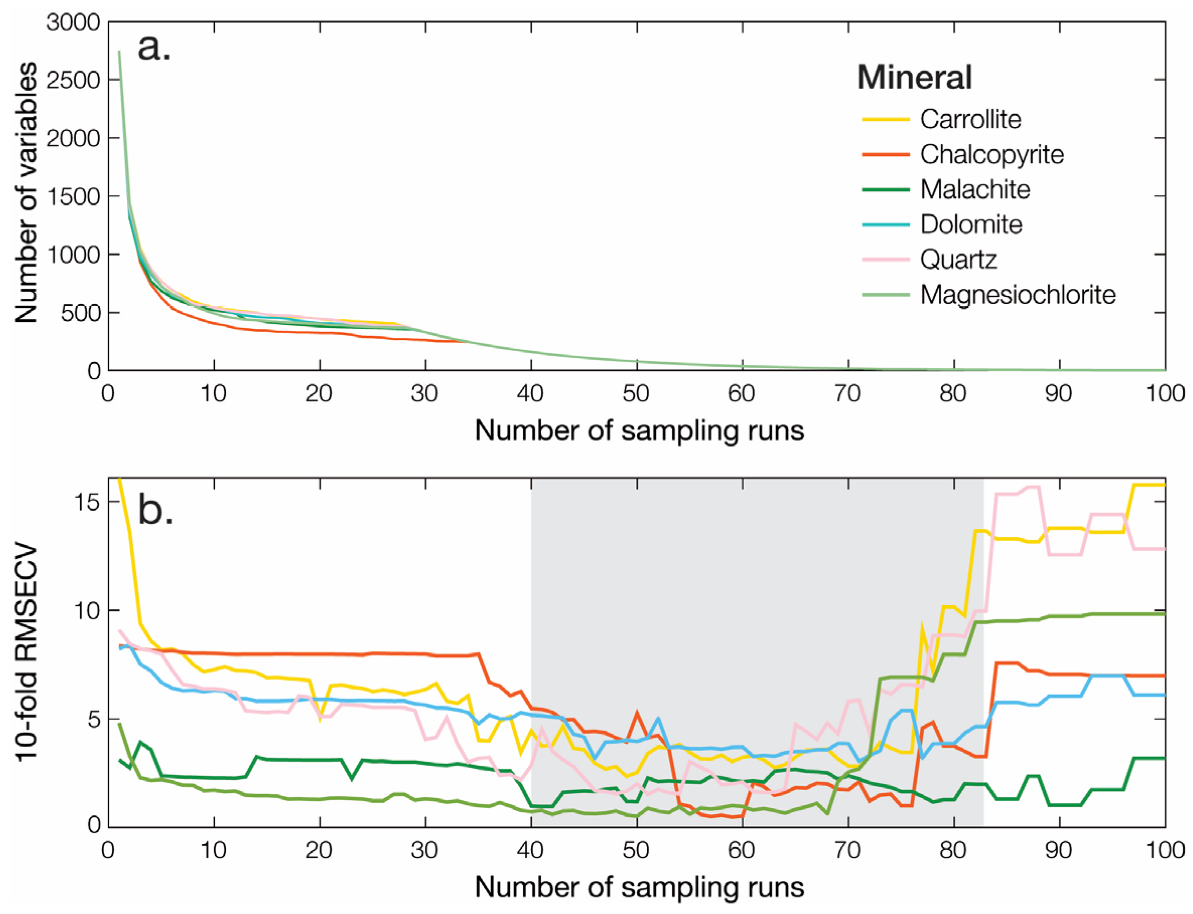
CARS sequentially select N subsets of wavelengths from N Monte Carlo sampling runs in an iterative and competitive manner based on the importance level of each variable. In each sampling run, a fixed ratio of samples is first randomly selected to establish a calibration model.

III.

A two-step procedure, including exponentially decreasing function (EDF)-based enforced wavelength selection and adaptive reweighted sampling-based competitive wavelength selection, is then adopted to select the key variables based on the regression coefficients.

IV.

Finally, a 10-fold cross validation is applied to choose the optimal subset of variables with the lowest RMSECV.

Ultimate multivariate predictive models validation was performed by test set validation which is considered to be the only correct validation method in chemometrics [69,73]. In this study, test set validation is performed by splitting the samples into a calibration set and a validation set with an 8:2 ratio, respectively. Dataset partitioning into calibration and validation subsets for the first PLS-R (step I) was performed using the SPXY (sample set partitioning based on joint X–y distances), an alternative to the Kennard–Stone algorithm which allows partitioning the dataset according to their differences in both X and y spaces [74]. Alternatively, for the second PLS-R after the CARS algorithm, partitioning was performed using SPXYE (sample set partitioning based on joint X–y-e distances), an improved version of the SPXY method. This method also takes into account the error of the preliminary PLS-R predictive model (e) for data partitioning by choosing the samples according to X, y and e spaces [75]. While most partitioning strategies aim to choose a representative training set, the algorithms were used to allocate samples to the training and validation set alternatively, therefore ensuring the representativity of both subsets.

The performance of the models was evaluated in terms of RMSE and determination coefficient (R²), pertaining to a fitted linear regression model between predicted versus reference mineral grades, for both the calibration set (RMSEC, R_c²) and the validation set (RMSEP, R_p²). In addition, the RMSECV of the 10-fold cross validation used for the selection of the optimal number of LVs in the PLS-R model is also considered. Spectral pre-processing techniques, PLS-R models, and variable selection were performed using Matlab^® (version R2018b, MathWorks Inc., The Aztec, MA, USA). The CARS algorithm is included with LibPLS toolbox [76], available online: http://www.libpls.net/ (accessed on the 10 September 2020).

3. Results

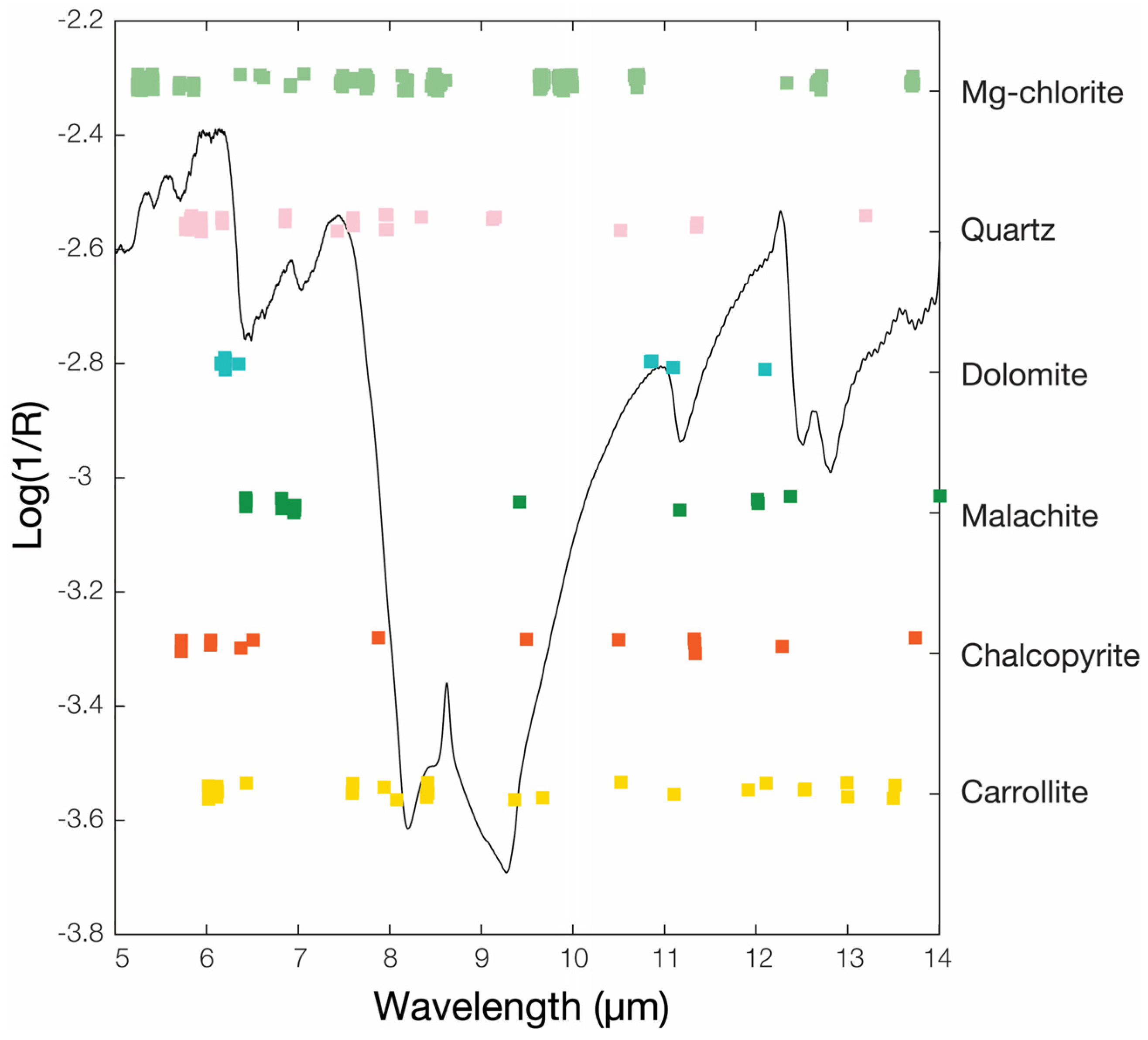
3.1. Feature Identification

The relatively homogenous zones observed within some thin sections, where one mineral is clearly dominant (>90 wt.%), can be used to establish reference FTIR spectra for the minerals present in the samples. For this purpose, FTIR spectra relating to the relatively homogeneous tiles in QEMSCAN fieldscan images were used (Scale 2, Figure 2). The reference spectra of five major minerals and the corresponding QEMSCAN fieldscan tiles of the area from which these were measured are presented in Figure 4. The reference spectra obtained for pure (>99 wt.%) malachite display multiple reststrahlen features. The main features include peaks at 6.62 μm and 7.17 μm, caused by C-O stretching, a peak at 9.52 μm due to OH vibration and a shoulder followed by a peak at 12.20 μm, both due to OCO bending [77,78]. An almost pure (88 wt.%) carrollite tile enabled the determination of a reference spectrum for carrollite, which display a maximum feature at 9.37 μm. Although FTIR spectra for carrollite are scarce in the literature, the position of the maximum feature is in agreement with the metal-sulphide maximum reported in literature [46,79]. Equally, it is close to the feature located at 9.34 μm in the RRUFF database FTIR spectra for carrollite [80]. The purest QEMSCAN tile found for chlorite (69 wt.%) yields an FTIR spectrum with the one main feature at 9.65 μm attributed to Si-O stretching. The presence of numerous impurities (mainly quartz, carrollite and bornite) may explain the absence of the two features observed at 9.40 μm and 10.40 μm in previous studies [81] and reference spectra [46]. The most homogeneous (94 wt.%) dolomite QEMSCAN tile produced an FTIR spectrum with two reststrahlen features at 6.40 μm and 11.20 μm which are attributed to bending of the C–O bond. This is in agreement with previous studies and reference spectra [36,37,46]. The pure quartz spectrum obtained from relatively homogenous tile (95 wt.%) displays two reststrahlen features at 8.60 μm and 12.60 μm due to the stretching of the Si–O bond, similar to those observed in previous studies [37,46].

Analysis of the (almost) pure mineral spectra allows identification of the characteristic features of minerals of interest. However, the investigated core samples are composed of a mixture of those minerals plus some others for which no pure mineral spectra could be extracted. Hence, due to a high degree of band overlap, identification of pure mineral features and quantitative modal mineralogy requires the use of multivariate predictive methods such as PLS regression (PLS-R).

In this paper we use PLS-R for the quantification of a limited number of key minerals. Some minerals like heterogenite, which is one of the main cobalt carriers in oxide ores, have not been included as no satisfying results could be obtained due to an insufficient amount or dissemination and intergrowth with minerals having overlapping characteristics bands in the set of samples collected for this study.

3.2. Multivariate Analysis for Modal Mineralogy

3.2.1. Optimal Pre-Processing Sequence Selection

Following the recommendation of Rinnan et al. [60], the optimal pre-processing sequence was selected by applying a full-spectrum PLS-R on the FTIR dataset after smoothing, SNV, MSC, SG 1st derivative (SG 1d) and combinations of these. An optimal spectral window selection was first performed for the pre-processing sequence including a smoothing step, i.e., smoothing, SG 1st derivative and combination of the latter with SNV or MSC. For each mineral, selection of the optimal spectral windows is based on lowest RMSEP of the full spectra PLS-R model (

Table 1. Optimum spectral window for the pre-processing sequence including a smoothing step. These are selected based on lowest RMSEP of the full spectra PLS-R model for each mineral.

Mineral	Smooth	SG 1d	SNV + SG 1d	MSC + SG 1d
Carrollite	29	7	53	19
Chalcopyrite	75	7	9	3
Malachite	77	29	95	21
Dolomite	63	7	95	93
Quartz	75	19	17	13
Mg-chlorite	77	99	95	95

).

The performance of the PLS-R model for the different pre-processing sequences is summarised in

Table 2. Comparison of the full spectra PLS-R model performance as a function of the pre-processing sequence for each mineral using the averaged FTIR data. The model with the lowest root mean squared errors (RMSEs) product (RMSECV × RMSEC × RMSEP) are highlighted in bold.

Mineral	Index	Raw	S *	SNV	S + SNV	MSC	S + MSC	SG 1d *	SNV + SG 1d *	MSC + SG 1d *
Carrollite	RMSECV	8.864	8.863	10.269	10.706	12.926	9.694	14.064	9.685	12.875
	RMSEC	8.456	8.457	5.871	6.150	9.429	1.249	11.818	0.880	5.039
	RMSEP	13.069	13.068	13.062	13.159	13.777	15.434	4.435	4.372	14.454
Chalcopyrite	RMSECV	5.713	5.684	7.634	7.851	7.646	4.171	6.624	7.603	8.730
	RMSEC	2.634	2.729	0.818	0.771	6.302	0.721	4.085	0.002	1.168
	RMSEP	6.130	4.330	2.228	4.859	6.685	67.132	1.763	1.674	1.801
Malachite	RMSECV	2.266	3.758	3.656	4.029	38.395	44.748	2.300	3.643	2.707
	RMSEC	0.830	0.782	2.823	2.075	9.432	9.068	0.805	2.313	0.577
	RMSEP	12.871	6.488	6.579	4.088	5.083	7.480	1.120	2.080	131.531
Dolomite	RMSECV	5.994	6.491	7.032	7.213	5.156	7.360	5.447	7.010	9.211
	RMSEC	3.537	3.306	3.624	4.550	0.471	1.041	1.688	2.530	7.505
	RMSEP	7.134	7.328	9.640	24.575	42.731	10.085	5.426	4.851	11.432
Quartz	RMSECV	5.267	6.118	7.105	7.836	6.600	7.895	7.582	8.403	8.563
	RMSEC	3.008	3.232	1.289	3.377	4.014	4.688	2.399	0.203	3.809
	RMSEP	11.996	11.647	10.275	9.971	14.001	11.382	10.878	9.863	11.793
Mg-chlorite	RMSECV	5.387	5.292	2.900	2.561	4.364	4.467	3.450	2.487	4.026
	RMSEC	1.927	0.870	1.079	0.740	3.043	2.867	0.279	0.090	1.927
	RMSEP	15.637	12.523	13.625	16.757	12.305	3.991	0.974	2.189	4.088

* Smoothing, computed using the optimal spectra windows given in Table 1.

. Overall, good predictions are obtained with SG 1st derivative alone or combined with SNV (which include a smoothing step), whereas MSC appears to lead to less suitable models. The reason for these differences in PLS-R model performance between pre-processing sequences described in Table 2 is complex and may be related to the differences in the way in which characteristic features of each mineral are highlighted by the different pre-processing methods. For each mineral, the selection of the best pre-processing sequence was based on the lowest RMSEs of the full-spectra PLS-R model by comparing the product of the three RMSEs, i.e., RMSECV × RMSEC × RMSEP.

The relatively high RMSECV of certain full-spectra PLS-R models for some minerals may be explained by the redundancy or noise due to the use of the full FTIR spectra for the calculations and the relatively low number of samples used for this analysis. These points will be addressed in the following sections. First, the CARS method is applied to the optimised pre-processed spectra to reduce the number of variables used to build the PLS-R models.

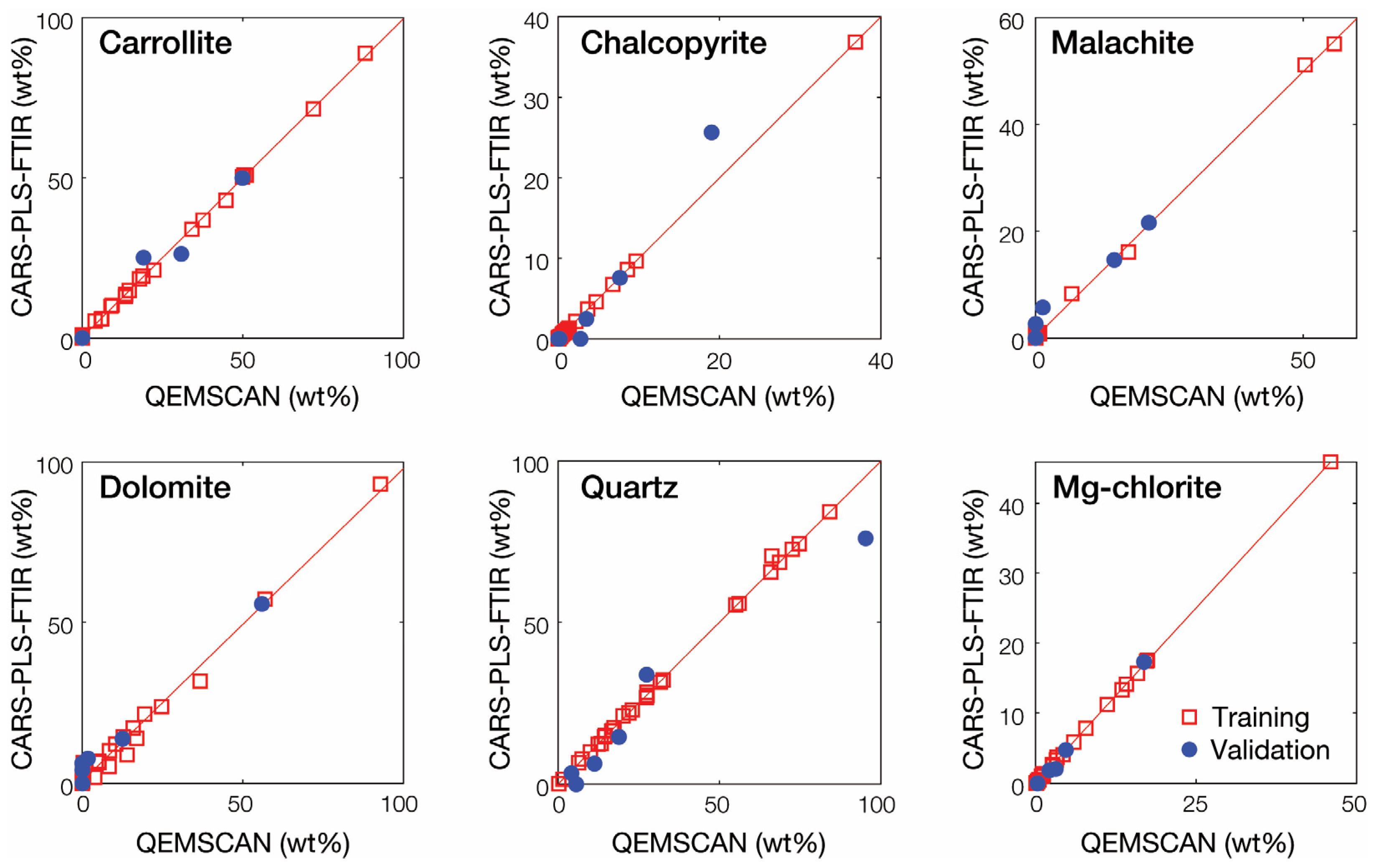
3.2.2. Competitive Adaptive Reweighted Sampling (CARS) Partial Least Squares Regression (PLS-R) on Average Spectra

Using the previously defined optimal pre-processing sequence for each mineral, PLS-R was first applied to the full spectrum and then to a selected sub-set of informative variables using the CARS algorithm.

Table 3. Summary statistics and performance indicators for the full spectra PLS-R and the CARS PLS-R calibrations using the average spectra data.

Minerals	Pre-Processing Procedure	nVAR *	nLVs *	Calibration Set (n = 28)			Validation Set (n = 6)
				RMSECV	${\mathit{R}}_{\mathit{C}}^2$	RMSEC	${\mathit{R}}_{\mathit{P}}^2$	RMSEP
Full spectrum PLS-R
Carrollite	SNV + SG 1d	2750	12	9.685	0.999	0.880	0.922	4.372
Chalcopyrite	SNV + SG 1d	2750	17	7.603	1.000	0.002	0.979	1.674
Malachite	SG 1d	2750	5	2.300	0.997	0.805	0.989	1.120
Dolomite	SG 1d	2750	7	5.447	0.993	1.688	0.975	5.426
Quartz	SNV + SG 1d	2750	13	8.403	1.000	0.203	0.947	9.863
Mg-chlorite	SG 1d	2750	18	3.450	0.999	0.279	0.859	0.974
CARS PLS-R
Carrollite	SNV + SG 1d	83	8	1.610	0.999	0.672	0.937	3.094
Chalcopyrite	SNV + SG 1d	40	13	0.312	1.000	0.054	0.976	3.378
Malachite	SG 1d	148	4	0.906	0.999	0.527	0.961	2.093
Dolomite	SG 1d	17	3	2.183	0.986	2.392	0.982	5.146
Quartz	SNV + SG 1d	72	10	1.159	1.000	0.405	0.961	9.002
Mg-chlorite	SG 1d	77	15	0.375	1.000	0.133	0.898	0.806

* nVar and nLVs denotes the number of selected variables and latent variables, respectively.

shows the summary statistics for both full-spectrum PLS-R and CARS PLS-R models for each mineral with corresponding pre-processing procedure, number of variables (nVAR), latent variables (nLVs), and model performance indexes. The full-spectrum PLS-R models display good performance with satisfactory validation results, i.e., $R_P^2$ of 0.922, 0.979, 0.989, 0.975, 0.947 and 0.859 with RMSEP of 4.372, 1.674, 1.120, 5.426, 9.863 and 0.974 for carrollite, chalcopyrite, malachite, dolomite, quartz and magnesiochlorite, respectively. However, it should be noted that a relatively high number of latent variables were used for some models, notably for carrollite (12 LVs), chalcopyrite (17 LVs), quartz (13 LVs) and magnesiochlorite (18 LVs). This increased model complexity may lead to overfitting issues. For example, there is a significant difference between RMSECV/RMSEC/RMSEP for carrollite, of 9.685, 0.880, respectively 4.372. This could be explained by the very large number of variables used for PLS-R, with the full spectra containing no less than 2760 variables. As a result, there is likely to be a significant amount of redundant information, uninformative data, or noise that affects the number of LVs in the PLS-R model and thus its performance.

In order to eliminate the uninformative variables, the CARS algorithm has been applied to the full spectra prior to PLS-R. CARS was performed for all minerals with a number of Monte Carlo sampling runs set to 100. This number is taken as the default value since the number of Monte Carlo sampling runs does not have a significant influence on the performance of CARS [70]. Figure 5 shows the evolution of the number of sampled wavelengths and the ten-fold RMSECV values with the increasing number of sampling runs. For all minerals, the number of sampled wavelengths decreases fast during the first stage of the EDF and then very slowly at the second stage of the EDF (Figure 5a). Simultaneously the RMSECV decreased, more progressively depending on the mineral, as the uninformative wavelengths were eliminated while the informative ones were retained up to a point where key wavelengths start to be removed, resulting in a sharp rise of the RMSECV value (Figure 5b). Even if not marked here, the optimal wavelengths subset, corresponding to a minimal RMSECV, is reached after 50–60 sampling runs for most minerals. Finally, 83, 40, 148, 17, 72 and 77 wavelengths were selected out of 2750 for carrollite, chalcopyrite, malachite, dolomite, quartz and magnesiochlorite, respectively.

An illustration of the informative wavelengths selected by CARS is shown in Figure 6. The selected wavelengths are widely distributed in the wavenumbers 6–14 µm, especially for Mg-chlorite and carrollite. Indeed, for some minerals, like malachite or quartz, the selected key wavelengths are mostly located in the region where their characteristic features are located. For other minerals like carrollite, the selected wavelengths are much broadly distributed. This may be attributed to the wide distribution of the characteristic features of the investigated minerals in this region (Figure 4), strong overlaps, high correlations in IR spectra, the broad reflectance features of some minerals [72,82] or the absence of a clear distinct feature as in the case of carrollite (Figure 4). In addition, mineralogical associations, and correlations between some mineral occurrences may also translate into characteristic wavelengths of these associated minerals being selected. Moreover, it should be noted that the multivariate analysis, unlike the reference work on which the characteristic features have been identified, is performed on the logarithm of the reciprocal reflectance, i.e., log(1/R), which may affect the relative strength of some spectral features that may appear stronger when the reflectance is plotted and thus the selected wavelength may differ slightly.

The results obtained with the CARS PLS-R models for each mineral are presented in Table 3 and Figure 7. As expected, the number of latent variables is reduced for all minerals even if some models still have a relatively high number of latent variables, notably chalcopyrite (13 LVs) and magnesiochlorite (15 LVs). Consequently, the CARS-PLS-R models display much lower RMSECV than the full-spectrum PLS-R models, with the RMSECV reducing by a factor of 2 to 9. The CARS PLS-R models display good performance with satisfactory validation results, i.e., $R_P^2$ of 0.937, 0.976, 0.961, 0.982, 0.961 and 0.898 with RMSEP of 3.094, 3.378, 2.093, 5.146, 9.002 and 0.806 for carrollite, chalcopyrite, malachite, dolomite, quartz and magnesiochlorite, respectively. Overall, the RMSEP obtained after CARS variable selection is also lower with the exception of chalcopyrite and malachite. Moreover, the regression models of all minerals, with the exception of quartz, have a smaller difference between RMSECV and RMSEP, suggesting a better performance and stability of the models [83].

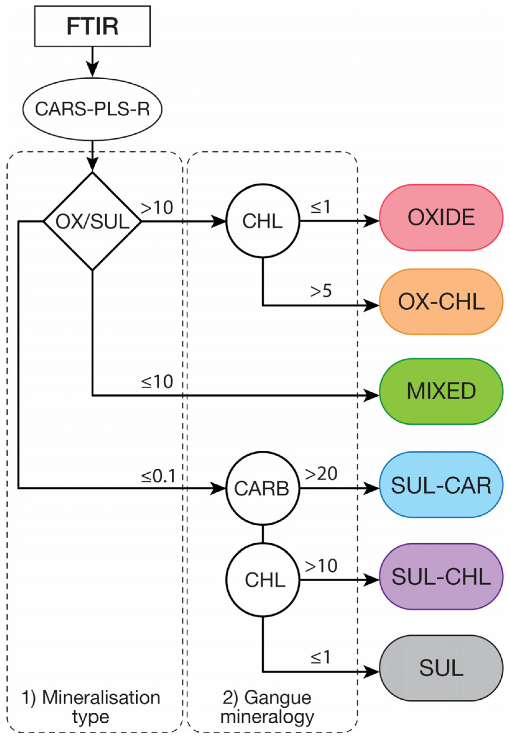
4. Discussion on the Potential Application to Geometallurgical Ore-Type Classification

Resource classification for sediment-hosted Cu-Co deposits are usually based on total Cu (TCu) and total Co (TCo) grades and occasionally on acid soluble Cu (AsCu) and Co (AsCo) content. The latter are usually determined by digesting (half-) core samples in a 10% sulphuric acid solution. The acid soluble AsCu and AsCo grades are taken to represent the presence of oxide Cu/Co-minerals while acid insoluble Cu (AiCu) and Co (AiCo), which follow from the difference between TCu/TCo and AsCu/AsCo, are used as a proxy for sulphide minerals [84]. However, not all oxide Cu/Co oxide minerals are readily soluble in sulphuric acid, they may be Co oxides locked in silicates or intergrown with clays and Fe-oxy-hydroxides [85], and secondary and some primary Cu/Co sulphide minerals are only partially soluble in acid [86]. This may affect the reliability of the aforementioned indicators as proxies for the amount of oxide/sulphide minerals [87]. Gangue acid consumption (GAC) and soluble iron content are alternative parameters that may be considered. While these indicators are good proxies to assess the recoverable Cu and Co during leaching, it requires an extensive test work program which is time-consuming and costly. In addition, these indicators are relevant for the leaching process but do not provide much information about the potential to recover AiCu and AiCo through flotation, which is also influenced by carrier and gangue minerals. All aforementioned indicators can be derived from modal mineralogy which drives the ore processing requirements (e.g., leaching versus flotation, leaching agent, flotation reagents, etc.) as the beneficiation route mainly depends on the state of the mineralisation (i.e., oxidised/weathered, mixed or reduced/sulphides) and the gangue mineralogy which influences acid consumption and flotation performance [12,26].

When developing a geometallurgical ore-type classification, it is important to capture essential elements which are relevant in terms of metallurgical and commercial significance [5,11]. A preliminary geometallurgical ore type classification for the investigated sediment-hosted Cu-Co deposit must include all the critical mineralogical features which not only influence but also define the mineral processing route: (1) overall Cu-Co mineral grades, (2) mineralisation type, i.e., oxide, sulphide or mixed, (3) gangue mineralogy, i.e., siliceous or carbonated, and (4) the presence of problematic minerals, i.e., chlorites, clays, talc, etc.

In sediment-hosted Cu-Co deposits, the oxide zones are usually processed through a classic leaching and solvent extraction-electrowinning (SX-EW) process, i.e., L/SX/EW while the sulphide ore is processed through a flotation route for the siliceous sulphide ore and a separate sulphidisation flotation route for the dolomitic sulphide ore and the mixed ore [14,20,21]. An example of a mineral-based geometallurgical ore-type classification scheme using modal mineralogy data obtained by FTIR-PLS-R is shown in Figure 8 with the corresponding variability in terms of ore mineralogy for each of these ore types (Figure 9). This classification proposal was kept as simple as possible while ensuring the metallurgical meaning of all geometallurgical ore types. It can be visualized as a decision tree for blending, stockpiling or mine planning which means that any ore pertaining to a given geometallurgical ore type should behave similarly during mineral processing. If not, the problematic ore type should be subdivided into relevant sub-types. Note that the values for the threshold presented in Figure 8 are only indicative and would need to be refined based on process performance.

The first stage of classification considers the type of mineralisation, i.e., oxide, sulphide or mixed, by calculating the ratio between oxide target minerals and sulphide target mineral grades. This can either be done using Cu/Co mineral grades determined through FTIR or by using the AsCu/AsCo data. Such information is critical as it defines the processing route to which the ore will be dispatched. The second stage of classification is undertaken on the gangue mineralogy, especially the presence of carbonates (dolomite, magnesite) and chlorites which are problematic for both leaching and flotation [12,23,26]. For this particular case study, the oxide horizons only display low grades of carbonate minerals. Hence, the oxide ore type is only subdivided in two categories, i.e., OXIDE for the common siliceous oxide ore and OX-CHL for the chlorite-rich oxide ore. The mixed ore (MIXED) typically display high carbonate grades (especially dolomite) and can contain relatively high chlorite grades as well [22]. Sulphide ore has been subdivided into three ore types: carbonate-rich (SUL-CAR), chlorite-rich (SUL-CHL), and a “common” sulphide ore (SUL).

While the ore types have distinct mineralogical compositions, there is some variation in mineral abundances within an ore type (Figure 9). In particular, the amount of target minerals (e.g., carrollite in sulphide ores, malachite in oxide ores) as well as gangue minerals (e.g., quartz in oxide ore types, Mg-chlorite in the mixed ore type) display a large amplitude of variation. This furthers strengthens the need, beyond ore-type classification, for accurate spatial quantification or the mineralogical variability within the deposit.

This study represents the first step in developing a geometallurgical model for the investigated Cu-Co mining operation. While process control typically aims to limit absolute variation in mineral recovery to say 0.5%, it can be shown through error propagation that this corresponds to an accuracy of 1 wt.% in the determination of mineral grades [26]. The lower level of accuracy may be fit-for-purpose in the context of geometallurgy [11]. Indeed, to establish geometallurgical domains and identify significant geometallurgical ore types, an accuracy of about ±5 wt.% (1σ) is considered to be adequate [88]. Results presented in Table 3 suggest that the level of accuracy for the determination of mineral grades used in the classification scheme presented in Figure 8 is sufficient for establishing geometallurgical domains.

The approach developed in this study, combining CARS-PLS-R to portable FTIR data, has the potential to be used as a geometallurgical tool with many advantages compared to currently available methods such as QXRD, automated mineralogy, element to mineral conversion, see

Table 4. Comparison of different available methods for modal mineralogy with the potential to be use for geometallurgical ore-type classification, using data from the literature, and the experience of the authors and experts.

Method	Quantitative X-ray Diffraction (QXRD)	Automated Mineralogy (AM)	Element to Mineral Conversion (EMC)	FTIR-CARS-PLS-R
Required data	Phase ID by XRD or other methods: crystal structure information of the phases	Mineralogy inferred from chemistry	Samples chemistry, Minerals chemistry Optional: approx. mineral grades (XRD)	-
Cost per sample (approx. US$)	100–200	200–500	~0 1	~0
Turnaround time (approx. hours)	3–7 2	16–32	~0 1	~0
Preparation time	1–3 2	8–20	-	-
Analytical time	1–3 2	4–8	~0 1	~0
Processing time	1–2	4	~0	~0
Experienced operator needed	Yes	Yes	No	No
Analysis	Bulk	Surface	Bulk	Surface/Bulk
Typical Precision (wt.%) 3	~2	≤1	~5	1–5
Typical closeness against AM (wt.%) 3	~3	-	1–10 4	5–10
Detection limit (wt.%) 3	0.2–5	≤0.01	0.01–0.14	1–5
Problem minerals	Amorphous phases, solid solution series	Polymorphs, nanocrystalline materials	Polymorphs	Ionic (e.g., halides)
Portable	Possible but less accurate	No	N/A	Yes
Calibration	No, internal standards can be used	Beam current (every 30 min), greyscale, EDS, beam alignment	Complex	Easy
Additional information obtained	Lattice parameters, <200 nm crystallite size, crystal structure details, amorphous content	Textural information, liberation, associations, grainsizes	Mineral chemistry	-
References	[54]	[29,89,90]	[11,91]	[53,54,92]

¹ Provided that the chemistry of the sample and the minerals therein is known. ² Sample preparation and analytical time may vary drastically depending on the mineral composition (e.g., iron content). ³ Precision, closeness against automated mineralogy (AM) and detection limits in absolute value. These values are only indicative and are mineralogy dependent, on only for the minerals that are actually quantified. ⁴ Also depends on the technique used to collect the sample chemistry.

. Indeed, portable FTIR can collect many spectra in a relatively short period of time, allowing accurate logging of mineralogy for many datapoints over large depth intervals along the borehole at the drilling site in real time or in the core shed [53]. This method is also quite cost-effective compared to existing methods as it does not require extensive sample preparation (e.g., preparation of bulk samples), and it can be applied directly to core samples and it has very low operational costs. The instrumentation cost is moderately high but still an order of magnitude lower that the aforementioned analytical methods. It should be noted that mineral conversion requires a consequent geochemical dataset covering all major elements and key trace elements, which may be prohibitive for small-scale operations. Portable FTIR is easy to operate, and the data processing and regression models can be routinely implemented to convert spectra into mineral grades. Ultimately, the choice of the method to be used for quantitative mineralogy depends on the required level of accuracy and the available budget, which varies per application. The results presented here suggest that geometallurgical ore-type classification and domaining using portable FTIR is a viable option.

While satisfactory results were obtained in this study, further investigation is required before considering this methodology as a universal solution for geometallurgical ore-type classification and mineral quantification. For instance, the effect of mineral grain size (as opposed to particle size) on the spectra when measured from a solid smooth surface like a core sample (as opposed to a bulk particulate material) remains unclear. Grainsize and texture are expected to influence the FTIR spectra and thus the outcome of the CARS-PLS-R and ultimately the geometallurgical ore-type classification. Hence, there may be ores, e.g., fine-grained intergrown mineralisation, for which the approach presented in this study may not apply. Other factors, such as a low abundance of highly IR responsive mineral (e.g., micas) in a matrix of low IR response minerals (e.g., feldspar, pyroxene), may bias the classification. Here, the major gangue minerals (quartz, dolomite) being IR responsive this issue was not investigated. Another important aspect not investigated in this study is the evolution of the RMSEP with mineral grades obtained by QEMSCAN. This would allow the effect of the latter on the closeness of the CARS-PLS-R FTIR method compared to QEMSCAN to be assessed, especially towards the low mineral abundances. The applicability of the approach described here may thus be limited to specific ores and deposits and further work is needed to define these limits of application.

5. Conclusions

The use of portable characterisation techniques such as FTIR is increasingly becoming a focus of research as it offers rapid and cost-effective approaches to mineral quantification, notably for geometallurgical applications. In this study, the application of FTIR to core samples from a sediment-hosted Cu-Co deposit from DRC enabled successful identification and quantification of major gangue minerals (quartz, dolomite, chlorite) and some sulphide minerals (chalcopyrite, carrollite). CARS-PLS-R applied to FTIR spectral data, using the corresponding QEMSCAN analysis as a reference, allowed prediction of gangue and target minerals grades with satisfactory validation results. While the overall accuracy of the generated regression models is an order of magnitude lower than those of bench-scale technology such as QXRD or automated mineralogy, this method could potentially be used for successful determination of ore types for mineral-based geometallurgical classification. This information may, therefore, be used to optimise resource efficiency and reduce risks linked to variable ore mineralogy. While the level of accuracy is sufficient for ore-type classification, further development is needed to reach the level of accuracy required to use the quantitative mineralogy data for process mineralogy applications.

References

1. Pell, R.; Tijsseling, L.; Goodenough, K.; Wall, F.; Dehaine, Q.; Grant, A.; Deak, D.; Yan, X.; Whattoff, P. Towards sustainable extraction of technology materials through integrated approaches. Nat. Rev. Earth Environ. 2021, 2, 665–679. [Google Scholar] [CrossRef]
2. Glass, H.J. Geometallurgy—Driving Innovation in the Mining Value Chain. In Proceedings of the Third AusIMM International Geometallurgy Conference (GeoMet) 2016, Perth, Australia, 15–16 June 2016; AusIMM: Melbourne, Australia, 2016; pp. 15–16. [Google Scholar]
3. Ashley, K.L.; Callow, M.I. Ore variability: Exercises in geometallurgy. Eng. Min. J. 2000, 201, 24–28. [Google Scholar]
4. Williams, S.R.; Richardson, J.M. Geometallurgical mapping: A new approach that reduces technical risks. In Proceedings of the Proceedings of 36th Annual Meeting of the Canadian Mineral Processors Conference, Ottawa, ON, Canada, 20–22 January 2004; CIM: Ottawa, ON, Canada, 2004; pp. 241–268. [Google Scholar]
5. Dehaine, Q.; Filippov, L.O.; Glass, H.J.; Rollinson, G.K. Rare-metal granites as a potential source of critical metals: A geometallurgical case study. Ore Geol. Rev. 2019, 104, 384–402. [Google Scholar] [CrossRef] [Green Version]
6. Dunham, S.; Vann, J.; Coward, S. Beyond Geometallurgy–Gaining Competitive Advantage by Exploiting the Broad View of Geometallurgy. In Proceedings of the The Firt AUSIMM International Geometallurgy Conference, Brisbane, Australia, 5–7 September 2011; pp. 5–7. [Google Scholar]
7. Dehaine, Q.; Michaux, S.P.; Pokki, J.; Kivinen, M.; Butcher, A.R. Battery minerals from Finland: Improving the supply chain for the EU battery industry using a geometallurgical approach. Eur. Geol. J. 2020, 5–11. [Google Scholar] [CrossRef]
8. Michaux, S.P.; O’Connor, L. How to Set Up and Develop a Geometallurgical Program—GTK Open Work File Report 72/2019; Geological Survey of Finland, Bulletin: Vuorimiehentie, Finland, 2020. [Google Scholar]
9. Dominy, S.C.; O’connor, L.; Parbhakar-Fox, A.; Glass, H.J.; Purevgerel, S. Geometallurgy—A route to more resilient mine operations. Minerals 2018, 8, 560. [Google Scholar] [CrossRef] [Green Version]
10. Lamberg, P. Particles—The bridge between geology and metallurgy. In Proceedings of the Conference in Mineral Engineering, Luleå, Sweden, 8–9 February 2011; pp. 1–16. [Google Scholar]
11. Lund, C.; Lamberg, P.; Lindberg, T. Practical way to quantify minerals from chemical assays at Malmberget iron ore operations—An important tool for the geometallurgical program. Miner. Eng. 2013, 49, 7–16. [Google Scholar] [CrossRef]
12. Dehaine, Q.; Tijsseling, L.T.; Glass, H.J.; Törmänen, T.; Butcher, A.R. Geometallurgy of cobalt ores: A review. Miner. Eng. 2021, 160, 106656. [Google Scholar] [CrossRef]
13. Crundwell, F.K.; du Preez, N.B.; Knights, B.D.H. Production of cobalt from copper-cobalt ores on the African Copperbelt—An overview. Miner. Eng. 2020, 156, 106450. [Google Scholar] [CrossRef]
14. Shengo, M.L.; Kime, M.-B.; Mambwe, M.P.; Nyembo, T.K. A review of the beneficiation of copper-cobalt-bearing minerals in the Democratic Republic of Congo. J. Sustain. Min. 2019, 18, 226–246. [Google Scholar] [CrossRef]
15. Macfarlane, A.S.; Williams, T.P. Optimizing value on a copper mine by adopting a geometallurgical solution. J. S. Afr. Inst. Min. Metall. 2014, 114, 929–936. [Google Scholar]
16. Cailteux, J.L.H.; Kampunzu, A.B.H.; Batumike, M.J. Lithostratigraphic position and petrographic characteristics of R.A.T. (“Roches Argilo-Talqueuses”) Subgroup, Neoproterozoic Katangan Belt (Congo). J. Afr. Earth Sci. 2005, 42, 82–94. [Google Scholar] [CrossRef]
17. Dewaele, S.; Muchez, P.; Vets, J.; Fernandez-Alonzo, M.; Tack, L. Multiphase origin of the Cu-Co ore deposits in the western part of the Lufilian fold-and-thrust belt, Katanga (Democratic Republic of Congo). J. Afr. Earth Sci. 2006, 46, 455–469. [Google Scholar] [CrossRef]
18. Van Langendonck, S.; Muchez, P.; Dewaele, S.; Kaputo Kalubi, A.; Cailteux, J.L.H. Petrographic and mineralogical study of the sediment-hosted Cu-Co ore deposit at Kambove West in the central part of the Katanga Copperbelt (DRC). Geol. Belg. 2013, 16, 91–104. [Google Scholar]
19. Jansen, M.; Taylor, A. Overview of gangue mineralogy issues in oxide copper heap leaching. In Proceedings of the ALTA 2003 Conference, Perth, Australia, 22–23 May 2003; pp. 701–714. [Google Scholar]
20. Bulatovic, S.M. Flotation of Oxide Copper and Copper Cobalt Ores. In Handbook of Flotation Reagents: Chemistry, Theory and Practice, Volume 2—Flotation of Gold, PGM and Oxide Minerals; Elsevier: Amsterdam, The Netherlands, 2010; pp. 47–65. ISBN 0444530290. [Google Scholar]
21. Shungu, T.; Vermaut, N.; Ferron, C.J. Recent trends in the Gecamines Copper-Cobalt flotation plants. Miner. Metall. Processing 1988, 163–170. [Google Scholar] [CrossRef]
22. Tijsseling, L.T.; Dehaine, Q.; Rollinson, G.K.; Glass, H.J. Flotation of mixed oxide sulphide copper-cobalt minerals using xanthate, dithiophosphate, thiocarbamate and blended collectors. Miner. Eng. 2019, 138, 246–256. [Google Scholar] [CrossRef]
23. Dehaine, Q.; Filippov, L.O.; Filippova, I.V.; Tijsseling, L.T.; Glass, H.J. Novel approach for processing complex carbonate-rich copper-cobalt mixed ores via reverse flotation. Miner. Eng. 2021, 161, 106710. [Google Scholar] [CrossRef]
24. Baum, W.; Ausburn, K. Daily process mineralogy: A metallurgical tool for optimized copper leaching. In Proceedings of the 5th international Seminar on Process Hydrometallurgy, Santiago, Chile, 10–12 July 2013; pp. 49–56. [Google Scholar]
25. Silvester, E.J.; Bruckard, W.J.; Woodcock, J.T. Surface and chemical properties of chlorite in relation to its flotation and depression. Miner. Processing Extr. Metall. 2011, 120, 65–70. [Google Scholar] [CrossRef]
26. Tijsseling, L.T.; Dehaine, Q.; Rollinson, G.K.; Glass, H.J. Mineralogical Prediction of Flotation Performance for a Sediment-Hosted Copper–Cobalt Sulphide Ore. Minerals 2020, 10, 474. [Google Scholar] [CrossRef]
27. Rietveld, H.M. A profile refinement method for nuclear and magnetic structures. J. Appl. Crystallogr. 1969, 2, 65–71. [Google Scholar] [CrossRef]
28. Pirard, E. Multispectral imaging of ore minerals in optical microscopy. Mineral. Mag. 2004, 68, 323–333. [Google Scholar] [CrossRef]
29. Gottlieb, P.; Wilkie, G.; Sutherland, D.; Ho-Tun, E.; Suthers, S.; Perera, K.; Jenkins, B.; Spencer, S.; Butcher, A.; Rayner, J. Using quantitative electron microscopy for process mineralogy applications. JOM 2000, 52, 24–25. [Google Scholar] [CrossRef]
30. Sutherland, D.N.; Gottlieb, P. Application of automated quantitative mineralogy in mineral processing. Miner. Eng. 1991, 4, 753–762. [Google Scholar] [CrossRef]
31. Gu, Y. Automated Scanning Electron Microscope Based Mineral Liberation Analysis An Introduction to JKMRC/FEI Mineral Liberation Analyser. J. Miner. Mater. Charact. Eng. 2003, 2, 33–41. [Google Scholar] [CrossRef]
32. Liipo, J.; Lang, C.; Burgess, S.; Otterstrom, H.; Person, H.; Lamberg, P. Automated mineral liberation analysis using INCAMineral. Process Mineral. 2012, 12, 1–7. [Google Scholar]
33. Hrstka, T.; Gottlieb, P.; Skála, R.; Breiter, K.; Motl, D. Automated mineralogy and petrology—Applications of TESCAN integrated mineral analyzer (TIMA). J. Geosci. 2018, 63, 47–63. [Google Scholar] [CrossRef] [Green Version]
34. Lund, C.; Lamberg, P. Geometallurgy—A tool for better resource efficiency. Eur. Geol. 2014, 37, 39–43. [Google Scholar] [CrossRef] [Green Version]
35. Gan, Y.; Yang, X.; Guo, Y.; Wu, S.; Li, W.; Liu, Y.; Chen, Y. The absorption spectra of H2O+and D2O+in the visible and near infrared region. Mol. Phys. 2004, 102, 611–621. [Google Scholar] [CrossRef]
36. Clark, R.N.; King, T.V.V.; Klejwa, M.; Swayze, G.A.; Vergo, N. High spectral resolution reflectance spectroscopy of minerals. J. Geophys. Res. 1990, 95, 12653–12680. [Google Scholar] [CrossRef] [Green Version]
37. Clark, R.N. Spectroscopy of Rocks and Minerals, and Principles of Spectroscopy. In Manual of Remote Sensing; Rencz, A.N., Ed.; John Wiley and Sons: New York, NY, USA, 1999; pp. 3–58. [Google Scholar]
38. Hunt, G.R. Spectral signatures of particulate minerals in the visible and near infrared. Geophysics 1977, 42, 501–513. [Google Scholar] [CrossRef] [Green Version]
39. Dalm, M.; Buxton, M.W.N.; Van Ruitenbeek, F.J.A.; Voncken, J.H.L. Application of near-infrared spectroscopy to sensor based sorting of a porphyry copper ore. Miner. Eng. 2014, 58, 7–16. [Google Scholar] [CrossRef]
40. Iyakwari, S.; Glass, H.J.; Rollinson, G.K.; Kowalczuk, P.B. Application of near infrared sensors to preconcentration of hydrothermally-formed copper ore. Miner. Eng. 2016, 85, 148–167. [Google Scholar] [CrossRef] [Green Version]
41. Tuşa, L.; Kern, M.; Khodadadzadeh, M.; Blannin, R.; Gloaguen, R.; Gutzmer, J. Evaluating the performance of hyperspectral short-wave infrared sensors for the pre-sorting of complex ores using machine learning methods. Miner. Eng. 2020, 146, 106150. [Google Scholar] [CrossRef]
42. Gaydon, J.W.; Glass, H.J.; Pascoe, R.D. Method for near infrared sensor-based sorting of a copper ore. J. Near Infrared Spectrosc. 2009, 17, 177–194. [Google Scholar] [CrossRef]
43. Viscarra Rossel, R.A.; Walvoort, D.J.J.; McBratney, A.B.; Janik, L.J.; Skjemstad, J.O. Visible, near infrared, mid infrared or combined diffuse reflectance spectroscopy for simultaneous assessment of various soil properties. Geoderma 2006, 131, 59–75. [Google Scholar] [CrossRef]
44. Thomson, J.L.; Salisbury, J.W. The mid-infrared reflectance of mineral mixtures (7–14 μm). Remote Sens. Environ. 1993, 45, 1–13. [Google Scholar] [CrossRef]
45. Salisbury, J.W.; Walter, L.S.; Vergo, N. Mid-InfraRed (2.1–25 um) Spectra of Minerals: First Edition, 1st ed.; United States Geological Survey: Reston, VI, USA, 1986.
46. Clark, R.N.; Swayze, G.A.; Wise, R.; Livo, K.E.; Hoefen, T.M.; Kokaly, R.F.; Sutley, S.J. USGS Digital Spectral Library 06. Available online: http://speclab.cr.usgs.gov/spectral.lib06 (accessed on 10 September 2020).
47. Clark, R.N. Spectral Properties of Mixtures of Montmorillonite and Dark Carbon Grains’ Implications for Remote Sensing Minerals Containing Chemically and Physically Adsorbed Water. J. Geophys. Res. 1983, 88, 635–645. [Google Scholar] [CrossRef]
48. Ramsey, M.S.; Christensen, P.R. Mineral abundance determination: Quantitative deconvolution of thermal emission spectra. J. Geophys. Res. Solid Earth 1998, 103, 577–596. [Google Scholar] [CrossRef]
49. Cooper, B.L.; Salisbury, J.W.; Killen, R.M.; Potter, E. Midinfrared spectral features of rocks and their powders. J. Geophys. Res. 2002, 107, 1–17. [Google Scholar] [CrossRef]
50. Henry, D.G.; Watson, J.S.; John, C.M. Assessing and calibrating the ATR-FTIR approach as a carbonate rock characterization tool. Sediment. Geol. 2017, 347, 36–52. [Google Scholar] [CrossRef] [Green Version]
51. Herres, W.; Gronholz, J.; Gronholtz, J.; Herres, W. Understanding FT-IR Data Processing—Part 1: Data Acquisition and Fourier Transformation. Comp. App. Lab 1984, 2, 216. [Google Scholar]
52. Harville, D.G.; Freeman, D.L.; Benefits, T.; Transform, F.; Spectroscopy, I. The Benefits and Application of Rapid Mineral Analysis Provided by Fourrier Transform Infrared Spectroscopy. In Proceedings of the SPE Annual Technical Conference and Exhibition—Society of Petroleum Engineers, Houston, TX, USA, 2–5 October 1988; pp. 141–151. [Google Scholar]
53. Ballard, B.D. Quantitative Mineralogy of Reservoir Rocks Using Fourier Transform Infrared Spectroscopy. In Proceedings of the SPE Annual Technical Conference and Exhibition—Society of Petroleum Engineers, Anaheim, CA, USA, 11–14 November 2007; pp. 1–8. [Google Scholar]
54. Ruessink, B.H.; Harville, D.G. Quantitative Analysis of Bulk Mineralogy: The Applicability and Performance of XRD and FTIR. In Proceedings of the SPE Formation Damage Control Symposium—Society of Petroleum Engineers, Lafayette, Louisiana, 26–27 February 1992; pp. 533–546. [Google Scholar]
55. Woods, J.; Gaafar, G.R. Application of Fourier Transform Infra-Red Spectroscopy in determination of reservoir properties. In Proceedings of the International Petroleum Technology Conference, Kuala Lumpur, Malaysia, 10–12 December 2014. [Google Scholar]
56. Craddock, P.R.; Herron, M.M.; Herron, S.L. Comparison of Quantitative Mineral Analysis By X-Ray Diffraction and Fourier Transform Infrared Spectroscopy. J. Sediment. Res. 2017, 87, 630–652. [Google Scholar] [CrossRef]
57. Woods, J. Application of Fourier Transform Infra-Red Spectroscopy (FTIR) for Mineral Quantification. Explore 2019, 1–6. Available online: https://www.appliedgeochemists.org/sites/default/files/documents/Explore%20issues/EXPLORE182%20March%202019.pdf.pdf (accessed on 10 September 2020).
58. Joassin, M.; Pirard, E. Application of Mid-infrared Reflectance Spectroscopy for the Identification of Minerals Present in Oil & Gas/Mining Exploration. In Proceedings of the Society Society of Geology Applied to Mineral Deposits (SGA) Conference, Québec City, QC, Canada, 20–23 August 2017. [Google Scholar]
59. Desta, F.S.; Buxton, M.W.N. The use of RGB Imaging and FTIR Sensors for Mineral mapping in the Reiche Zeche underground test mine, Freiberg. In Proceedings of the Real-Time Mining International Raw Materials Extraction Innovation Conference, Amsterdam, The Netherlands, 10–11 October 2017; van Gerwe, T., Hößelbarth, D., Eds.; Benndorf, Jorg: Amsterdam, The Netherlands, 2017; pp. 103–127. [Google Scholar]
60. Rinnan, Å.; van den Berg, F.; Engelsen, S.B. Review of the most common pre-processing techniques for near-infrared spectra. TrAC—Trends Anal. Chem. 2009, 28, 1201–1222. [Google Scholar] [CrossRef]
61. Barnes, R.J.; Dhanoa, M.S.; Lister, S.J. Standard normal variate transformation and de-trending of near-infrared diffuse reflectance spectra. Appl. Spectrosc. 1989, 43, 772–777. [Google Scholar] [CrossRef]
62. Savitzky, A.; Golay, M.J.E. Smoothing and Differentiation of Data by Simplified Least Squares Procedures. Anal. Chem. 1964, 36, 1627–1639. [Google Scholar] [CrossRef]
63. Goodall, W.R.; Scales, P.J. An overview of the advantages and disadvantages of the determination of gold mineralogy by automated mineralogy. Miner. Eng. 2007, 20, 506–517. [Google Scholar] [CrossRef]
64. Rollinson, G. Automated Mineralogy by SEM-EDS. In Encyclopedia of Geology; Elsevier: Amsterdam, The Netherlands, 2021; pp. 546–553. [Google Scholar]
65. Rollinson, G.K.; Andersen, J.C.Ø.; Stickland, R.J.; Boni, M.; Fairhurst, R. Characterisation of non-sulphide zinc deposits using QEMSCAN®. Miner. Eng. 2011, 24, 778–787. [Google Scholar] [CrossRef]
66. Geladi, P.; Kowalski, B.R. Partial least-squares regression: A tutorial. Anal. Chim. Acta 1986, 185, 1–17. [Google Scholar] [CrossRef]
67. Høskuldsson, A. Prediction Methods in Science and Technology; Thor Publishing: Copenhagen, Denmark, 1996. [Google Scholar]
68. Wold, S.; Sjöström, M.; Eriksson, L. PLS-regression: A basic tool of chemometrics. Chemom. Intell. Lab. Syst. 2001, 58, 109–130. [Google Scholar] [CrossRef]
69. Esbensen, K.H.; Guyot, D.; Westad, F.; Houmoller, L.P. Multivariate Data Analysis—In Practice: An Introduction to Multivariate Data Analysis and Experimental Design, 5th ed.; CAMO AS: Oslo, Norway, 2002; ISBN 8299333032. [Google Scholar]
70. Li, H.; Liang, Y.; Xu, Q.; Cao, D. Key wavelengths screening using competitive adaptive reweighted sampling method for multivariate calibration. Anal. Chim. Acta 2009, 648, 77–84. [Google Scholar] [CrossRef]
71. Fan, W.; Shan, Y.; Li, G.; Lv, H.; Li, H.; Liang, Y. Application of Competitive Adaptive Reweighted Sampling Method to Determine Effective Wavelengths for Prediction of Total Acid of Vinegar. Food Anal. Methods 2012, 5, 585–590. [Google Scholar] [CrossRef]
72. Luo, Q.; Yun, Y.; Fan, W.; Huang, J.; Zhang, L.; Deng, B.; Lu, H. Application of near infrared spectroscopy for the rapid determination of epimedin A, B, C and icariin in Epimedium. RSC Adv. 2015, 5, 5046–5052. [Google Scholar] [CrossRef]
73. Esbensen, K.H.; Geladi, P. Principles of proper validation: Use and abuse of re-sampling for validation. J. Chemom. 2010, 24, 168–187. [Google Scholar] [CrossRef]
74. Galvão, R.K.H.; Araujo, M.C.U.; José, G.E.; Pontes, M.J.C.; Silva, E.C.; Saldanha, T.C.B. A method for calibration and validation subset partitioning. Talanta 2005, 67, 736–740. [Google Scholar] [CrossRef] [PubMed]
75. Gao, T.; Hu, L.; Jia, Z.; Xia, T.; Fang, C.; Li, H.; Hu, L.H.; Lu, Y.; Li, H. SPXYE: An improved method for partitioning training and validation sets. Clust. Comput. 2018, 22, 1–10. [Google Scholar] [CrossRef]
76. Li, H.D.; Xu, Q.S.; Liang, Y.Z. libPLS: An integrated library for partial least squares regression and linear discriminant analysis. Chemom. Intell. Lab. Syst. 2018, 176, 34–43. [Google Scholar] [CrossRef]
77. Huang, C.K.; Kerr, P.F. Infrared study of the carbonate minerals. Am. Mineral. 1960, 45, 311–324. [Google Scholar]
78. Stoilova, D.; Koleva, V.; Vassileva, V. Infrared study of some synthetic phases of malachite (Cu2(OH)2CO3)-hydrozincite (Zn5(OH)6(CO3)2) series. Spectrochim. Acta—Part A Mol. Biomol. Spectrosc. 2002, 58, 2051–2059. [Google Scholar] [CrossRef]
79. Leppinen, J.O.; Basilio, C.I.; Yoon, R.H. In-situ FTIR study of ethyl xanthate adsorption on sulfide minerals under conditions of controlled potential. Int. J. Miner. Processing 1989, 26, 259–274. [Google Scholar] [CrossRef]
80. Lafuente, B.; Downs, R.T.; Yang, H.; Stone, N. The power of databases: The RRUFF project. In Highlights in Mineralogical Crystallography; Armbruster, T., Danisi, R.M., Eds.; De Gruyter (O): Berlin, Germany, 2015; pp. 1–29. ISBN 9783110417104. [Google Scholar]
81. Tappert, M.C.; Rivard, B.; Giles, D.; Tappert, R.; Mauger, A. The mineral chemistry, near-infrared, and mid-infrared reflectance spectroscopy of phengite from the Olympic Dam IOCG deposit, South Australia. Ore Geol. Rev. 2013, 53, 26–38. [Google Scholar] [CrossRef]
82. Blanco, M.; Cruz, J.; Bautista, M. Development of a univariate calibration model for pharmaceutical analysis based on NIR spectra. Anal. Bioanal. Chem. 2008, 392, 1367–1372. [Google Scholar] [CrossRef] [PubMed]
83. Wang, Y.; Jiang, F.; Gupta, B.B.; Rho, S.; Liu, Q.; Hou, H.; Jing, D.; Shen, W. Variable Selection and Optimization in Rapid Detection of Soybean Straw Biomass Based on CARS. IEEE Access 2018, 6, 5290–5299. [Google Scholar] [CrossRef]
84. Scheffel, R.E. Copper Heap Leach Design and Practice. In Mineral Processing Plant Design, Practice, and Control; Mular, A.L., Halbe, D.N., Barratt, D.J., Eds.; Society for Mining, Metallurgy, and Exploration (SME): Littleton, CO, USA, 1971; pp. 1571–1587. ISBN 978-0-87335-223-9. [Google Scholar]
85. Santoro, L.; Tshipeng, S.; Pirard, E.; Bouzahzah, H.; Kaniki, A.; Herrington, R. Mineralogical reconciliation of cobalt recovery from the acid leaching of oxide ores from five deposits in Katanga (DRC). Miner. Eng. 2019, 137, 277–289. [Google Scholar] [CrossRef]
86. Lasillo, E.; Schlittt, W.J. Practical Aspects Associated with Evaluation of a Copper Heap Leach Project. In Copper Leaching, Solvent Extraction, and Electrowinning Technology; Jergensen, I., Gerald, V., Eds.; Society for Mining, Metallurgy, and Exploration (SME): Littleton, CO, USA, 1999; pp. 123–138. ISBN 978-0-87335-183-6. [Google Scholar]
87. Kalichini, M.S. A Study of the Flotation Characteristics of a Complex Copper Ore. Master’s Thesis, University of Cape Town, Cape Town, South Africa, 2015. [Google Scholar]
88. Pitard, F.F. Pierre Gy’s Sampling Theory and Sampling Practice, Second Edition: Heterogeneity, Sampling Correctness, and Statistical Process Control; CRC Press: Boca Raton, FL, USA, 1993; ISBN 0849389178. [Google Scholar]
89. Leigh, G.M.; Sutherland, D.N.; Gottlieb, P. Confidence limits for liberation measurements. Miner. Eng. 1993. [Google Scholar] [CrossRef]
90. Pirrie, D.; Butcher, A.R.; Power, M.R.; Gottlieb, P.; Miller, G.L. Rapid quantitative mineral and phase analysis using automated scanning electron microscopy (QemSCAN); potential applications in forensic geoscience. Geol. Soc. Lond. Spec. Publ. 2004, 232, 123–136. [Google Scholar] [CrossRef]
91. Parian, M.; Lamberg, P.; Möckel, R.; Rosenkranz, J. Analysis of mineral grades for geometallurgy: Combined element-to-mineral conversion and quantitative X-ray diffraction. Miner. Eng. 2015, 82, 25–35. [Google Scholar] [CrossRef]
92. Chen, Y.; Furmann, A.; Mastalerz, M.; Schimmelmann, A. Quantitative analysis of shales by KBr-FTIR and micro-FTIR. Fuel 2014, 116, 538–549. [Google Scholar] [CrossRef]
Figure 1. Sample preparation procedure and correspondence between the thin section analysed by QEMSCAN and the mirrored sample analysed by Fourier transformed infrared (FTIR) spectroscopy.
Minerals 12 00015 g001
Figure 2. Schematic view of measurement workflow on the mirrored image on the drill core and corresponding QEMSCAN tiles on the thin section.
Minerals 12 00015 g002
Figure 3. Illustration of some spectra pre-processing methods. (a) Raw spectra, (b) smoothed spectra (window = 11), (c) standard normal transformed spectra, (d) multiplicative scattering corrected spectra, and (e) first derivative spectra of the selected core samples.
Minerals 12 00015 g003
Figure 4. Overview of normalized and smoothed single-mineral spectra obtained from the most homogenous zones (purity in wt.%) of the mirrored samples and corresponding tile on the fieldscan image obtained by QEMSCAN.
Minerals 12 00015 g004
Figure 5. Illustration of the CARS wavelength selection algorithm. (a) Number of sample variables as a function of the number of sampling iterations. (b) Ten-fold RMSECV as a function of the number of sampling iterations.
Minerals 12 00015 g005
Figure 6. Example of a key wavenumbers in the FTIR spectra selection by the CARS algorithm for all the investigated minerals with the averaged log(1/R) spectrum.
Minerals 12 00015 g006
Figure 7. Measured (QEMSCAN) vs. predicted plot of the CARS-PLS-R models for the investigated minerals after data processing using the average spectra data.
Minerals 12 00015 g007
Figure 8. Mineral-based geometallurgical ore type classification scheme proposal using modal mineralogy data obtained from CARS-PLS-R applied to FTIR. OX/SUL: ratio between the amount (in wt.%) of Cu-Co oxide and Cu-Co sulphide minerals, CARB: total amount (in wt.%) of carbonates (Dolomite, ankerite, magnesite) and CHL: amount (in wt.%) of chlorites. Classification thresholds are only indicative.
Minerals 12 00015 g008
Figure 9. Boxplots illustrating the modal mineralogy variability (in wt.%) in different ore types of the studied Cu-Co deposit, using the QEMSCAN analysis of the selected core samples.
Minerals 12 00015 g009