1. Introduction
In mineral exploration, magnetic data have traditionally been inverted to produce magnetic susceptibility models, which represent magnetization induced by the current magnetic field. This does not take into account, however, the remanent magnetization of the rocks produced by the ancient magnetic field. More information about rock formations and geological processes can be obtained by inverting magnetic data for magnetization vector, as opposed to magnetic susceptibility only. At the same time, increasing the number of inversion parameters (i.e., inverting for the scalar components of magnetization vector) increases the non-uniqueness of the inverse problem. We overcome this problem by jointly inverting multiple geophysical data sets. The total magnetic intensity (TMI) and airborne gravity gradiometry (AGG) data are typically gathered in coincident surveys, making them a natural choice for joint interpretation.
Over the last decade, significant efforts were made by many researchers to develop the methods of magnetic data inversion in the presence of remanent magnetization. To include both induced and remanent magnetization, one needs to model the distribution of magnetization vector within the rock formation rather than the distribution of scalar susceptibility alone. This approach was used by [
1,
2] to invert TMI data. This enables explicit inversion of the magnetization direction and amplitude, rather than just the magnetization amplitude only (e.g., [
3]). Ellis et al. [
4] reported further progress in the solution of this problem; they introduced a technique for regularized inversion for the magnetization vector. From the magnetization vector, one can recover information about both the remanent and induced magnetization. A detailed overview of the published papers can be found in the comprehensive review paper by Y. Li [
5], where one can find a long list of publications on the subject. We reference the interested readers to this publication for more information about the recent advances in 3D inversion of magnetic data in the presence of significant remanent magnetization
The results presented in the cited papers, however, illustrate the practical difficulties of the inversion related to the fact that, in this case, one has to determine from the observed scalar TMI data three unknown components of the magnetization vector within each cell instead of one unknown value of susceptibility. The main problem is with the increased practical non-uniqueness associated with the inverse problem.
In order to reduce the non-uniqueness of the inverse problem, we use a method of direct inversion of the magnetic data for the magnetization vector based on applying a Gramian stabilizer in the framework of the regularized inversion [
6]. To this end, we also present a method of joint inversion of AGG and TMI data in the presence of remanent magnetization. We consider two different approaches to the joint inversion. The first approach is joint inversion with Gramian constraints [
7], where the structural correlation of the different model gradients is enforced. The Gramian constraint is analogous to the cross-gradients method [
8]; however, whereas the cross-gradients approach typically relies on an approximation, the Gramian constraint utilizes an exact analytical formula for the gradient direction of the parametric functional, which guarantees rapid convergence of the inverse solution [
9].
The second approach presented is joint inversion with a joint focusing stabilizer [
10,
11], which enforces null-space sparsity in both models via a modified minimum support constraint. It is well known that the focusing stabilizers minimize the areas with anomalous physical properties (in the case of the minimum support stabilizer) or the areas where major changes in physical properties occurs (in the case of the minimum gradient support stabilizer). The joint focusing stabilizers force the anomalies of different physical properties to either overlap or experience a rapid change in the same areas, thus enforcing the structural correlation.
To illustrate both of these approaches, we present a case study of the joint inversion of the AGG and TMI data, which were collected over the Thunderbird V-Ti-Fe deposit in the Ring of Fire area of Ontario, Canada. The Ontario Geological Survey (OGS) and the Geological Survey of Canada (GSC) collaboratively gathered the airborne data with the Fugro Airborne Surveys gravity gradiometer and magnetic system between 2010 and 2011. Appropriate filters are applied to the data, i.e., reduction-to-pole (RTP) and deep regional trend removal. The filtered RTP data were used to invert the susceptibility model. The original TMI data with the removed regional trend were inverted for the magnetization vector. Standalone inverse models are produced using a single datum, i.e., AGG or TMI only, yielding standalone models to compare and contrast to the jointly inverted models and to produce appropriate model weights used in the joint inversions.
We compare and contrast the 3D density, magnetic susceptibility, and magnetization vector models of the Thunderbird V-Ti-Fe deposit obtained from standalone, Gramian, and joint-focused inversions. Application of both joint inversion methodologies to these data has resulted in 3D models of subsurface formations that have sharper geospatial boundaries and stronger structural correlations than the standalone inverted models. The Gramian constraint approach yielded the highest level of numerical structural correlation. The joint focusing approach provided similar results but was significantly faster and easier to implement.
2. Forward Modeling of the Gravity and Magnetic Data
2.1. Gravity Forward Modeling
The gravity field can be computed from the gradient of the gravity potential
:
where
is the universal gravity constant;
and
are the observation and integration points, respectively;
is the density; and the gravity potential,
has the following form:
The second spatial derivatives of the gravity potential
form a symmetric gravity gradient tensor,
where
The expressions for the gravity tensor components can be written as follows:
where kernels
are equal to:
One can use the point-mass approximation to calculate Formula (5) in discretized form by considering each cell as a point mass [
12].
2.2. Magnetic Forward Modeling and Magnetization Vector
The earth’s current magnetic field is the vector sum of contributions from two main sources: the background magnetic field due to the dynamo in the earth’s liquid core, and the crustal field due to magnetic minerals. Conventional magnetic inversion methods produce a 3D magnetic susceptibility model from the magnetic vector field,
, or from the total magnetic intensity (TMI) data,
. This is an effective tool for targeting magnetic mineralization; however, the following assumptions must generally be made: (1) there is no remanent magnetization, (2) self-demagnetization effects are negligible, and (3) the magnetic susceptibility is isotropic (e.g., [
13,
14,
15,
16]).
Under these assumptions, the intensity of magnetization,
, is linearly proportional to the inducing magnetic field,
,
where
is the magnetic susceptibility and
is the unit vector along the direction of the inducing field. Given the inclination (
), declination (
), and azimuth (
) from the International Geomagnetic Reference Field (IGRF), the direction of the inducing magnetic field can be computed as follows (assuming that the
axis is directed eastward, the
axis has a positive direction northward, and the
axis is downward):
Thus, the anomalous magnetic field can be presented in the following form:
In airborne magnetic surveys, the total magnetic intensity (TMI) field is measured, which can be computed approximately as follows:
In the general case, however, the earth’s magnetic field is nonstationary over geological time, meaning that the direction of magnetization in rock formations may differ from the direction of today’s magnetic field. This is due to several factors, i.e., geomagnetic reversals and wandering poles. The ancient magnetization can be particularly useful when exploring magnetic structures such as kimberlites, dykes, iron-rich ultramafic pegmatitoids (IRUP), platinum group element (PGE) reefs, and banded iron formations (BIF). Moreover, remanence can also be used to determine the age of intrusive or alteration events.
By inverting for magnetization vector, one can take into account the effects of self-demagnetization, anisotropy, and remanent magnetization. To include both induced and remanent magnetization, we need to model on the magnetization vector rather than the scalar susceptibility. This modifies Equation (7) as follows:
where
has two parts: induced,
, and remnant,
magnetizations:
Therefore, Equation (10) should also be modified:
One can compute the volume integral in Equation (13) in closed form for magnetic susceptibility. We can also evaluate the volume integral numerically with sufficient accuracy using single-point Gaussian integration with pulse basis functions provided the depth to the center of the cell exceeds twice the dimension of the cell [
12].
3. Inversion for Magnetization Vector Using Gramian Constraints
In this section, we present a summary of the principles of the robust inversion for the magnetization vector using Gramian constraints.
It is well-known that the regularized solution of the geophysical inverse problem can be formulated as minimization of the Tikhonov parametric functional,
where
is the magnetization vector and
is a misfit functional defined as the squared
norm of the difference between the predicted,
and observed,
data,
In the last formula, is the forward modeling operator for the magnetic problem described by a discrete form of Equation (13).
Notations
in Equation (14) indicate in compact form that we can use any one of three types of stabilizing functionals,
, based on minimum norm, minimum support, and minimum gradient support constraints, respectively. These stabilizers are determined as follows [
17]:
and
where
is a focusing parameter, which can be selected using an L-curve method [
9].
The minimum norm stabilizer, minimizes the variations of the solutions, , from the a priori model, . The minimum support stabilizer, minimizes the volume occupied by the anomalous magnetization, while the minimum gradient support stabilizer, selects the inverse models with sharp boundaries between the formations with different magnetic properties. Thus, by selecting the proper stabilizing functionals, the user may emphasize different properties of the inverse models. The minimum norm stabilizer usually results in relatively smooth distributions of magnetization, while the focusing stabilizers, and generate models with sharp boundaries. We use regularized inversion with focusing stabilization, as this recovers models with sharper boundaries and higher contrasts than the regularized inversion with smooth (e.g., minimum norm) stabilization.
The minimization problem (14) can be solved using a variety of optimization methods. For improved convergence and to avoid any matrix inversions, we minimize Equation (14) using the re-weighted regularized conjugate gradient (RRCG) method. We refer the reader to [
17] for further details of this method.
Inverting for the magnetization vector is a more challenging problem than inverting for scalar magnetic susceptibility, because we have three unknown scalar components of the magnetization vector for every cell. At the same time, in the case of induced magnetization, there is an inherent correlation between the different components of the magnetization vector. In order to ensure a smooth change in the direction of the magnetization vector, we impose a similar condition by requiring that the different components of the magnetization vector should be mutually correlated as well. The results of numerical model experiments and case studies show that this approach to regularization ensures a robust inversion for magnetization vector.
It was demonstrated in [
7] that one can enforce the correlation between the different model parameters by using the Gramian constraints. Following the cited paper, we have included the Gramian constraint in Equation (14) as follows:
where
is the
length vector of magnetization vector components;
is the
length vector of the
component of magnetization vector,
;
is the
-length vector of the effective magnetic susceptibility, defined as the magnitude of the magnetization vector,
Functional
is the Gramian constraint,
where
denotes the
inner product operation [
9].
Using the Gramian constraint (21), we enhance a direct correlation between the scalar components of the magnetization vector with , which is computed at the previous iteration of an inversion and is updated on every iteration. The advantage of using the Gramian constraint in the form of Equation (21) is that it does not require any a priori information about the magnetization vector (e.g., direction and the relationship between different components) since the amplitude, is computed at the previous iteration. On the first iteration, the scalar components are determined independently
The minimization problem (19) is solved using the re-weighted regularized conjugate gradient (RRCG) method. Details of the RRCG method and conjugate gradient derivations for the parametric functional (19) can be found in [
9,
17].
4. Joint Inversion of Gravity and Magnetic Data
4.1. Gramian Joint Inversion
In a case of joint inversion of gravity and magnetic data, the geophysical inverse problem is given by the following set of operator Equations:
where
is the density model,
is the magnetization vector model,
are the forward modeling operators,
are the data, and the superscript
indicates the gravity and magnetic problems, respectively. Operators
are usually represented as discrete forms of the corresponding integral expressions (5) and (13) for gravity gradient and TMI fields, respectively.
We should note that the units and scales of the density and magnetization vector are very different. Therefore, in practical applications, we should operate with the normalized, dimensionless model parameters [
9]:
where
are the corresponding linear operators of the model weighting. A trivial example of these operators could be just division of the model parameters by their upper or lower bounds,
or
or by the corresponding interval of the model parameters distribution,
This simple normalization makes the normalized parameters vary on the same scale. In a general case, the model weights can be defined based on integrated sensitivities, which will be discussed in details below.
Similarly, different data sets, as a rule, have different physical dimensions as well. Therefore, it is convenient to consider dimensionless weighted data,
defined as follows:
where
are the corresponding linear operators of the data weighting.
The solutions of geophysical inverse problems (22) are typically ill-posed [
9]. A corresponding well-posed problem can be constructed by applying regularization and minimizing a parametric functional using the conjugate gradient method. In this case, misfit and stabilizing terms, each corresponding to the gravity gradiometry and magnetic data, are incorporated into a joint parametric functional, which is subject to the Gramian structural constraint:
where
and
are the regularization parameters, responsible for degrees of smoothing/focusing
) of the models and enforcing similarities (
) between the density and magnetization distributions, produced by a joint inversion. We use an adaptive algorithm of selecting these parameters, described in [
9].
The misfit terms are defined as follows,
where
are the weighted predicted data:
The stabilizing terms, are based on minimum norm, minimum support, and minimum gradient support constraints, respectively, as defined by Formulas (16)–(18).
The Gramian term is defined by the following formula,
where
is the gradient of the density model,
are the gradients of the scalar components of magnetization vector, and
denotes the
inner product operation [
9]. Minimization of the Gramian aligns the model gradients, which in turn enforces the structural similarity of the shared earth model.
In a case of structural Gramian constraints defined by Formula (28), one can normalize the gradient vectors by their length:
with expression for Gramian (28) taking the form:
This normalization enforces the correlations of the unit vectors in the gradient directions, thus resulting in the structural similarity between the models representing density and magnetizations of the rock formations.
4.2. Joint Focusing Inversion
Another approach to joint inversion can be based on a joint total variation functional [
18], or on joint focusing stabilizers, e.g., minimum support and minimum gradient support constraints [
10,
11]. It is well known that the focusing stabilizers minimize the areas with anomalous physical properties (in the case of the minimum support stabilizer) or the areas where major changes in physical properties occur (in the case of the minimum gradient support stabilizer). The joint focusing stabilizers force the anomalies of different physical properties to either overlap or experience a rapid change in the same areas, thus enforcing the structural correlation. We will demonstrate these properties in the model study presented in our paper.
The AGG and TMI data misfit terms are incorporated in the joint parametric functional and subject to the joint focusing stabilizers:
The data misfit functionals are defined as above in Equation (26). The terms
and
are the joint stabilizing functionals, based on minimum support and minimum gradient support constraints, respectively [
10,
11].
For example, a joint minimum support stabilizer can be introduced as follows:
where
is the focusing parameter, which can be selected using an L-curve method [
19]. In a similar way, we can introduce a joint minimum gradient support functional (JMGS):
The joint focusing constraint is not applied until the data misfit functionals have been sufficiently minimized (e.g., ). This avoids the introduction of inversion artifacts arising from the focusing constraint.
4.3. Representation of a Stabilizing Functional in the Form of a Pseudo-Quadratic Functional
In this and the following sections, for simplicity, we will drop the tilde sign above the dimensionless weighted data and model parameters, assuming that they have already been normalized according to Formulas (23) and (24).
The focusing stabilizing functionals introduced above can be represented as pseudo-quadratic functionals of the model parameters [
9,
17]:
where
is a linear operator of the product of the model parameters function,
and the weighting function,
which may depend on
If operator
does not depend on
, we obtain a quadratic functional, i.e., a minimum norm-stabilizing functional
In general cases,
may even be a nonlinear function of
like the minimum support (32) or minimum gradient support (33) functionals. In these cases, the functional
, determined by Formula (34), is not quadratic. That is why we call it a “pseudo-quadratic” functional. However, it was shown in [
9,
17] that presenting a stabilizing functional in a pseudo-quadratic form enables the development of a unified approach to regularization with different stabilizers and simplifies the solution of the regularization problem.
For example, the joint minimum support functional,
can be written as follows:
where
is a linear operator of the multiplication of the model parameter function,
by the following weighting function,
:
For the joint minimum gradient support functional,
we assume
and find
where
is a linear operator of the multiplication of the model parameter function,
by the following weighting function,
and
is a small number similar to a focusing parameter
Using the pseudo-quadratic form (37) of stabilizing functional, we can present the corresponding parametric functional (31) as follows:
Therefore, the parametric functional introduced by Equation (31) can be minimized in the same manner as a conventional Tikhonov parametric functional. The only difference is the introduction of some variable weighting operator,
, which depends on the model parameters. A practical technique of minimizing the parametric functional (39) is based on application of the re-weighted regularized conjugate gradient (RRCG) method. Interested readers can find a detailed description of the RRCG algorithm in [
9].
4.4. Data and Model Weights
Data and model weights are critical in both joint inversion scenarios presented, because they ensure that both inverse problems (gravity and magnetic) converge towards a satisfactory solution at roughly the same rate. Appropriate data and model weights also ensure that the models do not unduly bias one another where no structural corellation exists. As such, in both joint inversion scenarios, two levels of data and model weighting are employed. Initial data weights are given by the following function of the errors:
where
are the relative errors, and
are the absolute error floors. These intial data weights are used in standalone and joint inversion; however, in the joint inversions, data weights are further scaled by the initial data misfit for each data set:
where
are the initial misfits. The matrices of initial model weights are given by the integrated sensitivity [
9,
17]:
where
is the Fréchet derivative of
and
is the transposed matrix. In the joint inversions, the model weights are further scaled by normalization with the maximum model contrast obtained from standalone inversions:
where
are the density and magnetization models obtained from standalone (separate) inversions, and
are the background density and magnetization values.
The constants
are adaptively and monotonically reduced to ensure stable convergence towards a satisfactory solution [
9,
12]. The inversion is halted when both misfit terms have been minimized to the noise level.
5. Model Study
To illustrate the developed methods, we present the results of their application to synthetic gravity gradiometry and TMI data generated for a two-body model shown in
Figure 1. The bodies are both parallelepipeds of dimensions 200 × 50 m, situated at 50 m and 100 m depths. The left body has physical properties of 0.3 g/cm
3, −0.06 A/m in the X direction, and 0.06 A/m in the Z direction. The right body has physical properties of 0.4 g/cm
3, 0.06 A/m in the X direction, and 0.06 A/m in the Z direction. The magnetization vectors for both bodies have inclinations of
and opposing declinations of
and
, or east/west. The inducing field has inclination
and declination
. The Gxx, Gyy, and Gzz gravity gradiometry components and TMI data are simulated at equidistant stations laterally spaced at 25 m with a flight height of 30 m, also shown in
Figure 1. All data are contaminated with 5% Gaussian noise.
We have inverted the synthetic data using the standalone and joint inversions, introduced in the previous sections. Note that, in this model study and in the following case study, we have inverted magnetic data for all three scalar components of the magnetization vector, which is the principal distinguished feature of the developed method in comparison to the conventional approach based on inversion for magnetic susceptibility only. At the same time, there are several possible approaches for how to calculate the joint focusing functionals required for joint inversion. For example, we can consider three joint focusing stabilizers—each involving a scalar component of magnetization vector and density—or jointly focus the amplitude of magnetization vector and density. We have found that jointly focusing the dominant scalar component and density works the best. Therefore, we only include the vertical component of magnetization vector, in the focusing stabilizers. Based on the results of the standalone magnetization vector inversion, the vertical component of magnetization vector, is dominant in this area. As such, the joint focusing term includes only the density, and the vertical component of magnetization vector, to reduce non-uniqueness.
The inversion domain was discretized into rectangular cells with a horizontal cell size of 25 × 25 m and with 20 logarithmically spaced vertical layers for a total cell count of ~45,000. All inversions were terminated when both data sets reach the simulated noise level .
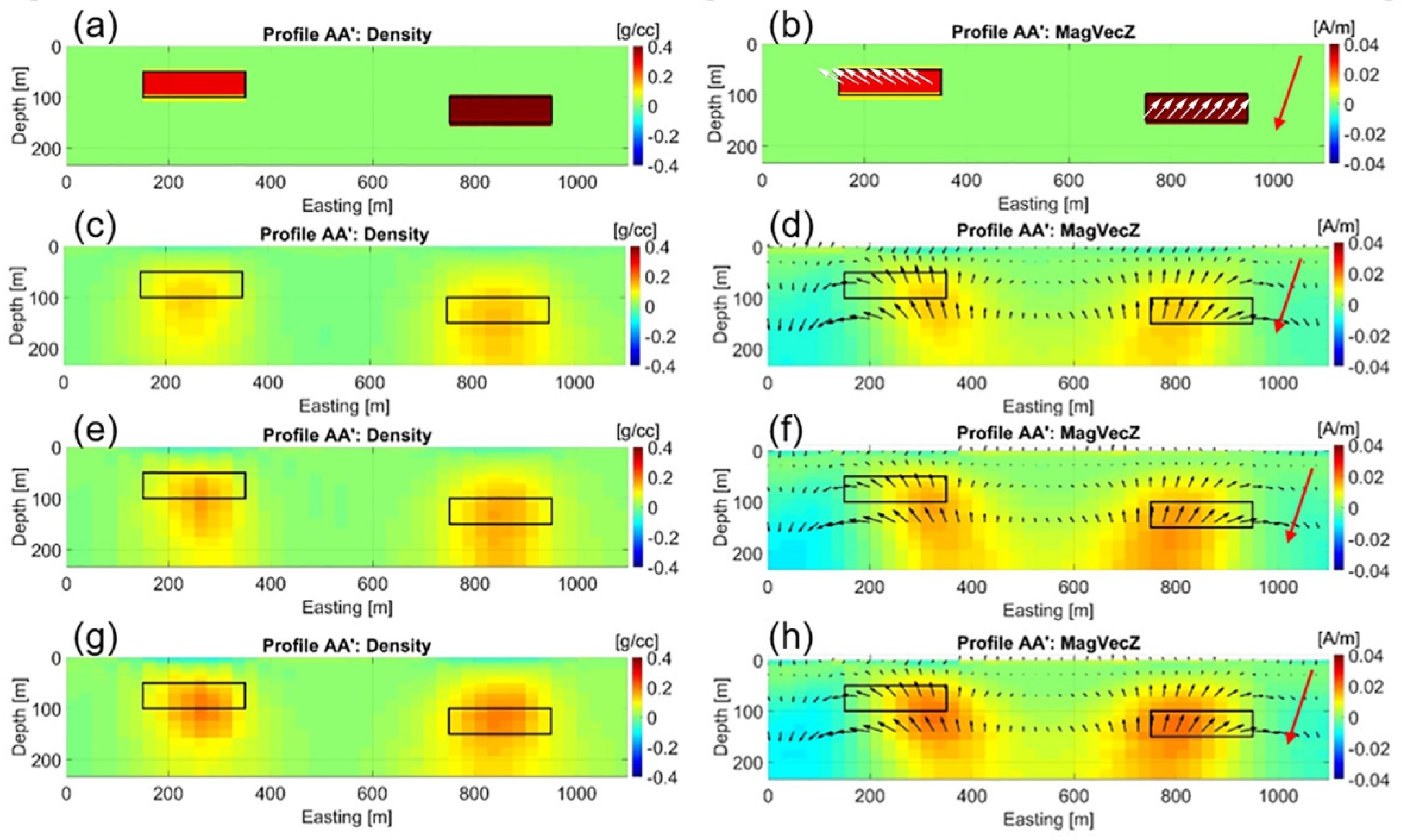
Vertical sections of the true model and inverse solutions from standalone and joint inversions are shown in
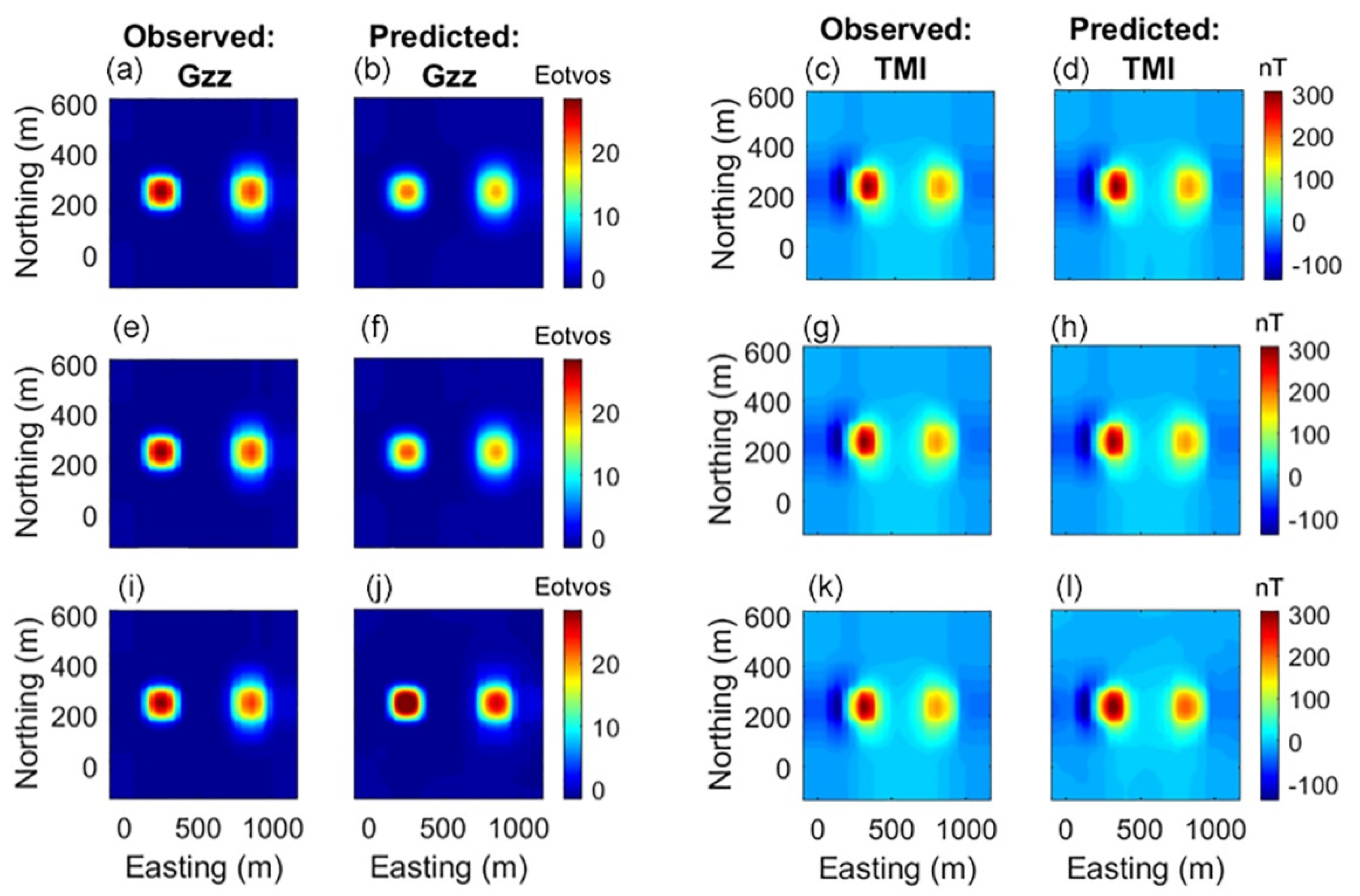
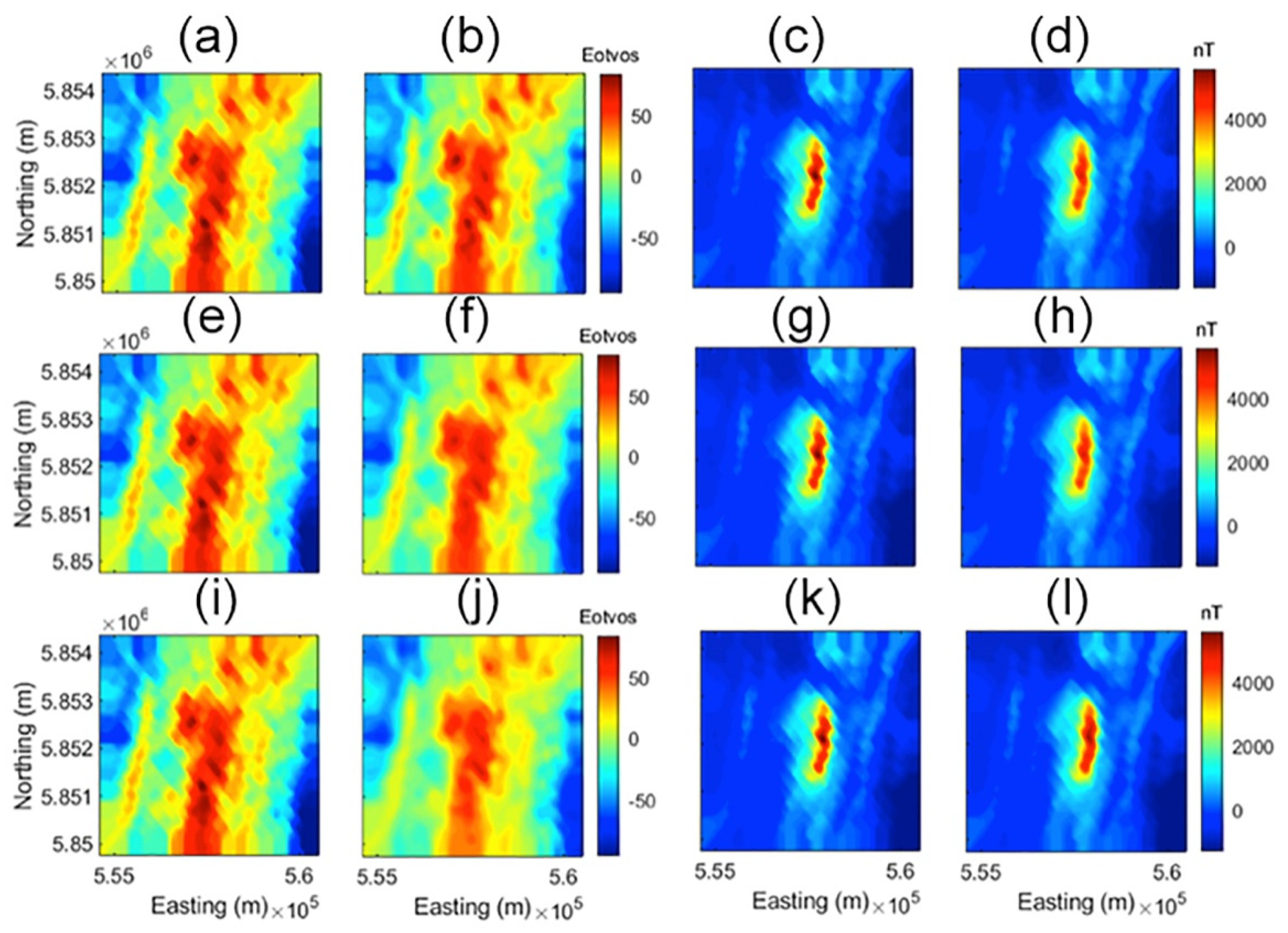
Figure 2. They illustrate that the joint inversions produce a better image of the model than the standalone inversions while maintaining a similar level of data misfit. Observed and predicted data for the Gzz component of gravity gradiometry and the TMI data for the various inversion scenarios are shown in
Figure 3. We can see that the joint-focused inversion slightly improves data fidelity compared to the other inversion types. Between the joint inversion scenarios, the Gramian and joint-focused inversions arrive at similar models and data fits; however, inversion with joint focusing is three times faster with respect to both iterations required and computational speed.
6. Case Study of Joint Inversions of Airborne Gravity Gradiometer (AGG) and Magnetic Data
6.1. Regional Geology in the Ring of Fire
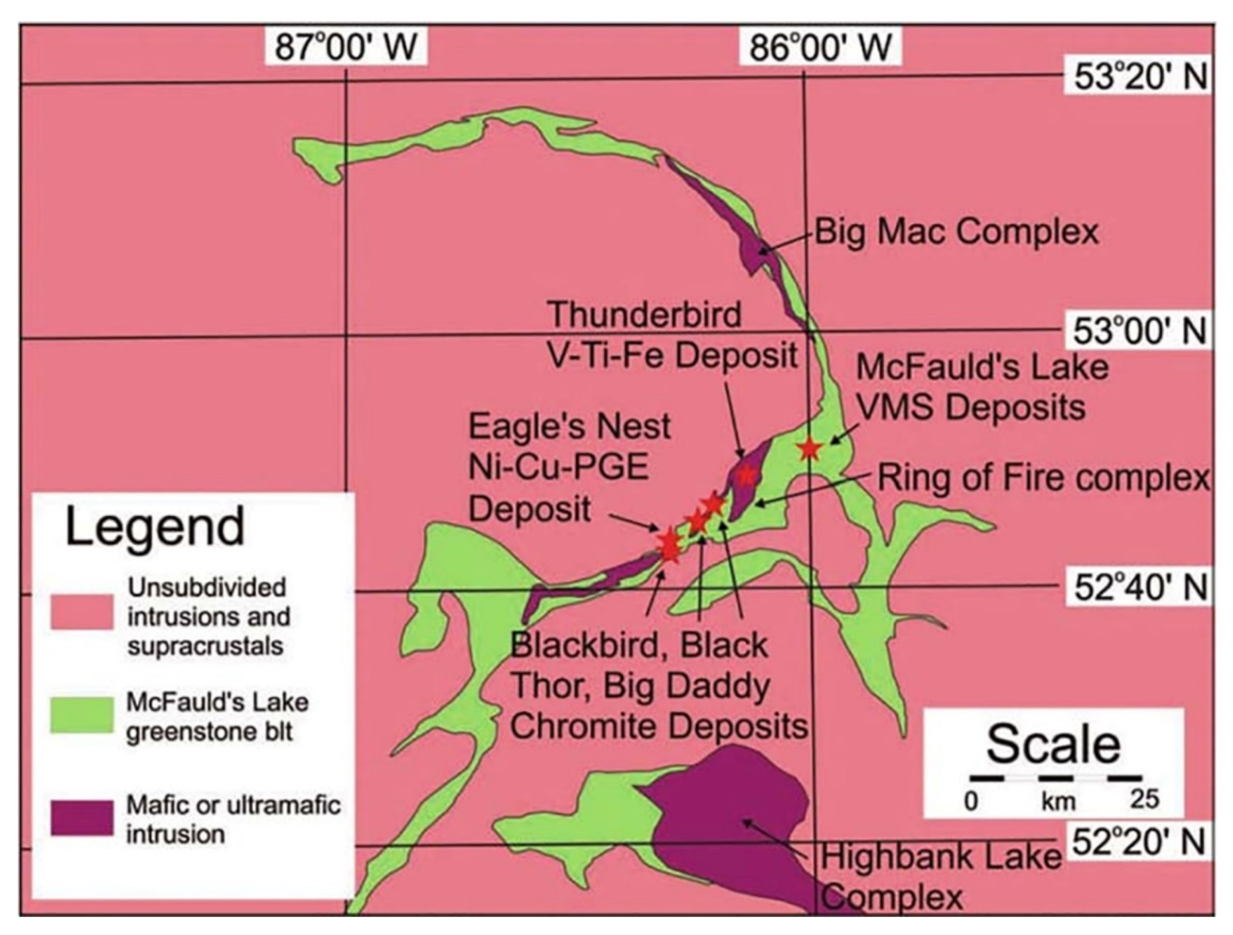
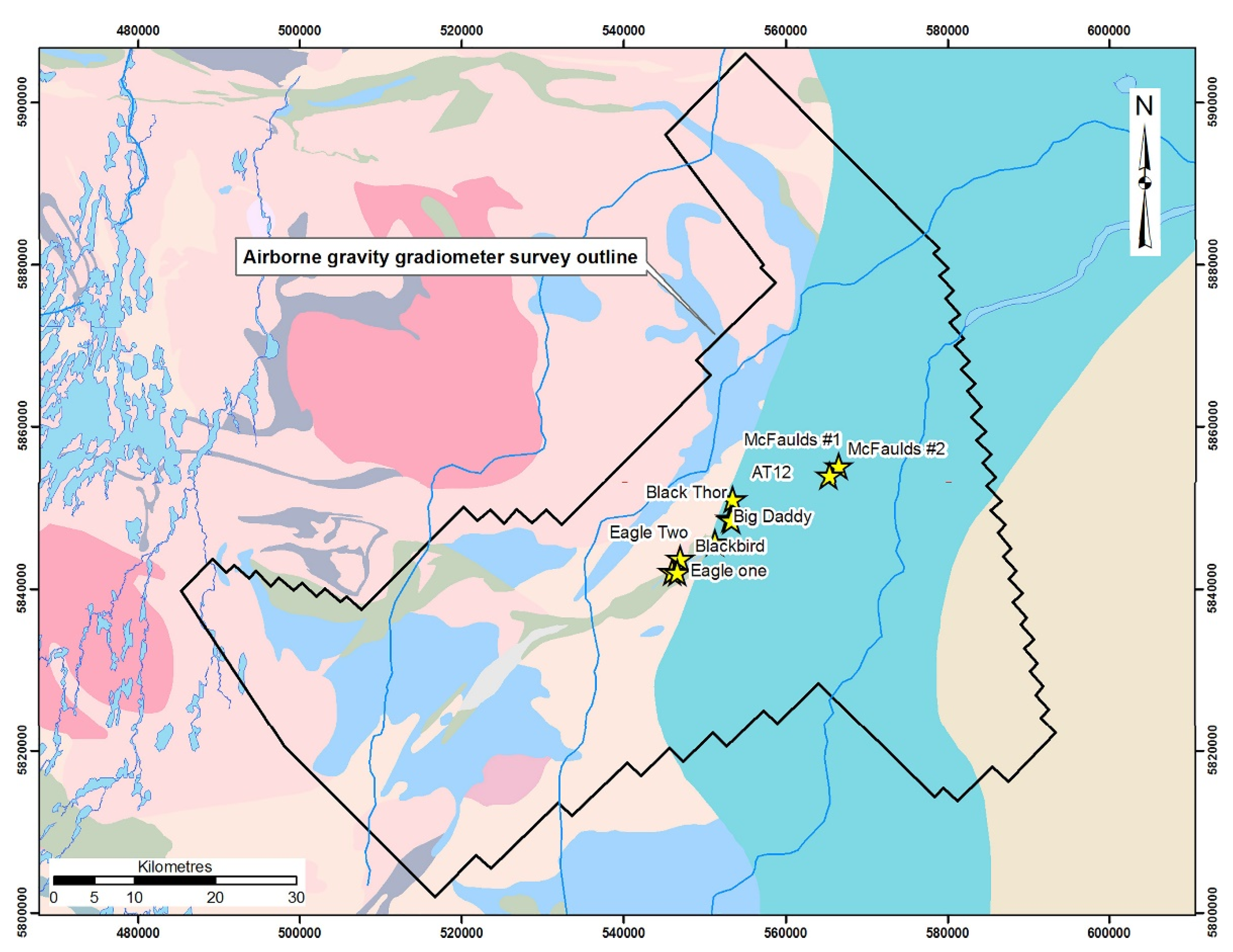
McFaulds Lake covers the Ring of Fire intrusive complex located in the James Bay lowlands of northwestern Ontario. Ring of Fire is a roughly north–south trending Archean green belt (
Figure 4) consisting of mafic and ultramafic rocks. Due to flat topography and Paleozoic carbonate rocks cover, the area was not extensively studied until the early 2000s, when, as a part of kimberlite exploration campaign, McFaulds volcanic massive sulfide (VMS) deposits were discovered. The recognition that the area hosts a greenstone belt has triggered an exploration rush which resulted in three major types of economic mineral deposit discoveries, including magmatic Ni-Cu-PGE, magmatic chromite mineralization, and volcanic massive sulfide mineralization.
The Ring of Fire complex is primarily composed of mafic metavolcanic flows, felsic metavolcanic flows, and pyroclastic rocks. The Thunderbird deposit is associated with one of the numerous layered mafic-to-ultramafic intrusions, which trend subparallel with and obliquely cut the westernmost part of the belt, close to a large granitoid batholith lying west of the belt [
21]. These layered intrusions are associated with high-grade Ni-Cu-PGE, Chromite, and V-Ti-Fe deposits, with Thunderbird being the latter.
6.2. Airborne Gravity and Magnetic Surveys
In the exploration rush of the mid-2000s, there were numerous smaller-scale exploration projects performed; however, the overall picture of the area was lacking. In order to map regional geology and locate further potential mineral resources, an airborne geophysical survey was carried out in the McFaulds Lake region between 2010 and 2011 using the Fugro Airborne Surveys system. Both airborne gravity gradiometer (AGG) and magnetic data were collected. This project was collaboratively operated between the Ontario Geological Survey (OGS) and the Geological Survey of Canada (GSC).
Figure 5 shows the McFaulds Lake region survey block. The survey parameters included:
- (1)
Flight height: 100 m
- (2)
Line spacing: 250 m
- (3)
Line km: 19,733
- (4)
Area: 4577 m2
- (5)
AGG: Falcon
- (6)
Magnetic: single sensor
6.3. Thunderbird Deposit
The Thunderbird deposit consists of semi-massive vanadium- and titanium-enriched magnetite, which corresponds to a strong gravity and magnetic anomaly. Noront Resources, owner of the claim, estimates the ore body at 1.6 km long, 400 m wide, and 500 m deep, based on gravity and magnetic data and limited core drilling. This deposit has not been developed yet, and a more detailed analysis is lacking.
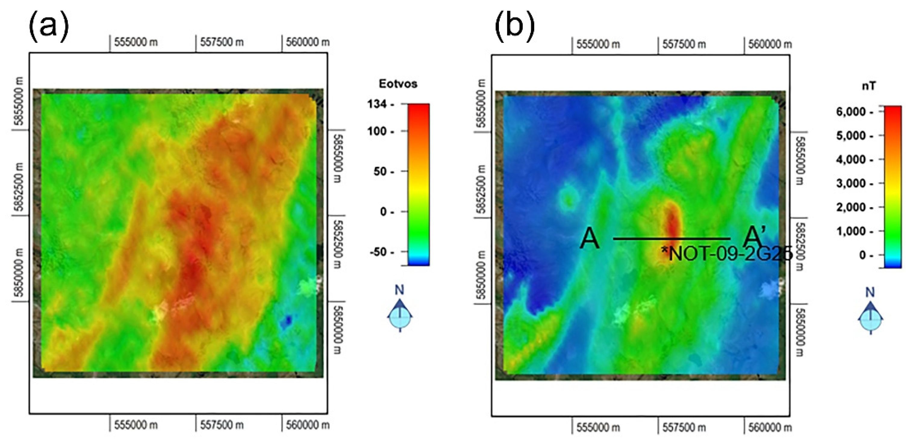
We have inverted the Gxy, Gxx, Gyy, and Gzz gravity gradient components and TMI data separately and jointly. As discussed above, the filtered RTP magnetic data were used for susceptibility inversion, while the inversion for magnetization vector was based on the TMI data with the removed regional trend. As an example, panel (a) of
Figure 6 shows the Gzz component of the observed AGG data, while panel (b) presents the filtered TMI data map of the Thunderbird area. The deposit is assumed to be a semi-massive V-Ti-enriched magnetite with an approximate volume of 0.32 km, which is based on potential field data analysis and limited core drilling.
The inversion grid was discretized with a 50 × 50 m horizontal spacing and a logarithmic vertical discretization ranging from 25–150 m. The total number of cells inverted was ~250,000 cells. A 16-core Intel Xeon workstation with 128 GB memory was used to run all of the inversions. The total inversion runtime was ~10 min for the standalone AGG and TMI inversions, ~15 min for the joint inversion with joint focusing stabilization, and ~45 min for the joint inversion with Gramian constraints.
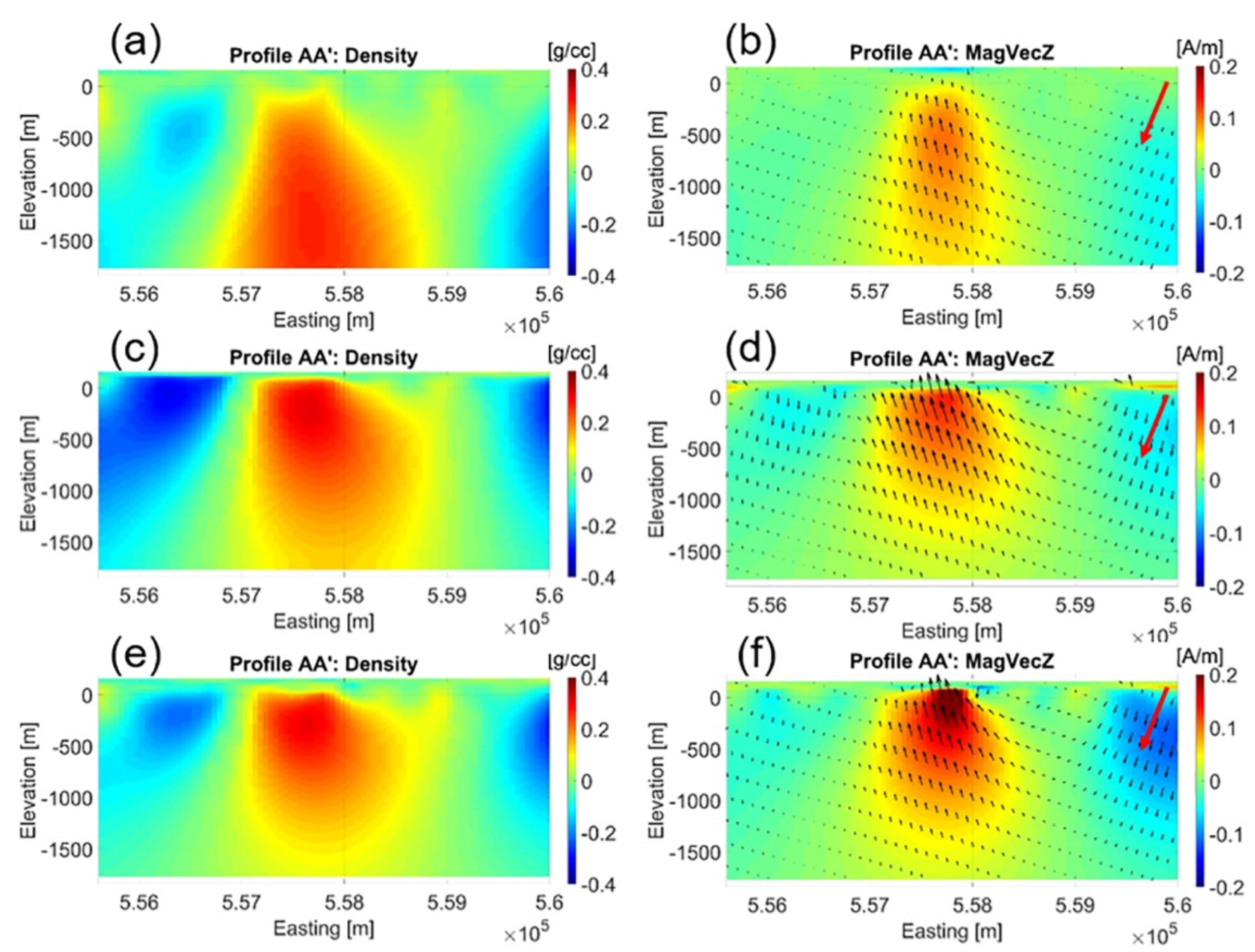
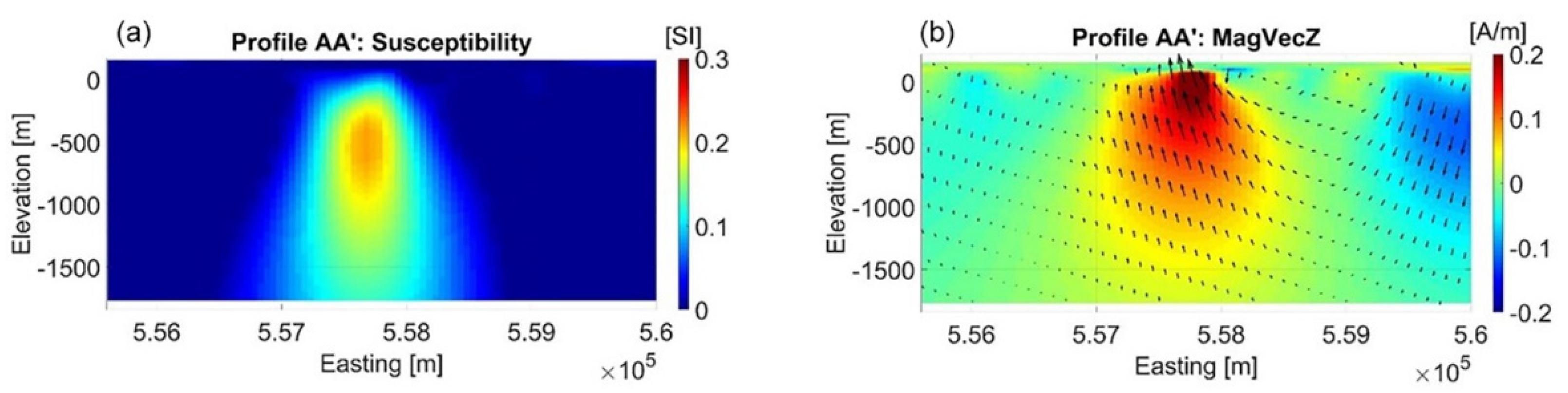
A comparison of vertical sections of the 3D models obtained from the various inversion methodologies is shown in
Figure 7. It is clear that the models obtained from a joint inversion with either Gramian or joint focusing constraints have sharper geospatial boundaries and a higher degree of structural correlation, when compared to the models obtained from standalone inversions. It is important to note that all inverted 3D models share the same level of data misfit.
We have included both the full magnetization vector and the inducing field direction in the magnetic panels for clarity. Drill hole NOT-09-2G25, drilled by Noront Resources Limited in 2009 [
22] and situated in the center of these profiles, found a gabbro schist unit from 21–462 m containing magnetite and titanomagnetite with concentrations up to 10% and smaller pockets containing up to 50% magnetite. This matches quite well with the jointly inverted results. Moreover, an iron formation with up to 20% magnetite concentration was found at 166–170 m which may be what the focused inversion is resolving in the near surface.
A comparison of selected observed and predicted data is shown in
Figure 8. All inversion methodologies reach an excellent data fit.
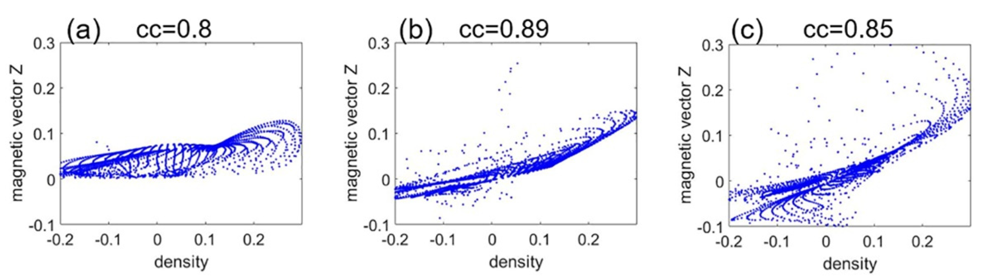
Figure 9 shows model parameter cross plots for the different inversion scenarios. Additionally, the correlation coefficient was calculated for the density model versus the vertical component of the magnetization vector and is summarized in
Table 1.
Figure 10 and
Figure 11 show a comparison between the results of the susceptibility-only inversion and magnetization-vector inversion. The left panel in
Figure 10 shows the vertical section of the inverse model for susceptibility inversion, while the right panel shows the vertical section of the inverse model for magnetization vector inversion. The small black arrows in the right panel represent the magnetization vectors, while the color bar reflects the vertical component of magnetization.
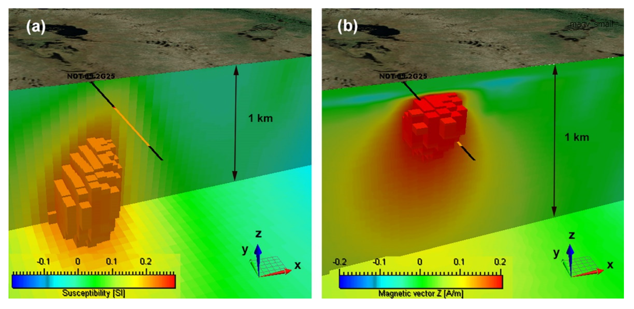
Figure 11 shows a comparison of 3D inverse models with drilling results. The left panel (a) presents the volume image of the inverse susceptibility, while the right panel (b) shows a similar image of the vertical component on the magnetization vector. The black–yellow–black solid line is the borehole drilled in the survey area. The yellow color indicates the mineralization zone confirmed by drilling. One can see that the image produced by inversion for the magnetization vector correctly represents the location of the mineralization zone. In other words, the volume images also show that you can better pinpoint anomalous bounds with magnetization vector in the presence of remanent magnetization for the Thunderbird Vanadium-Titanium target in Ontario, Canada.
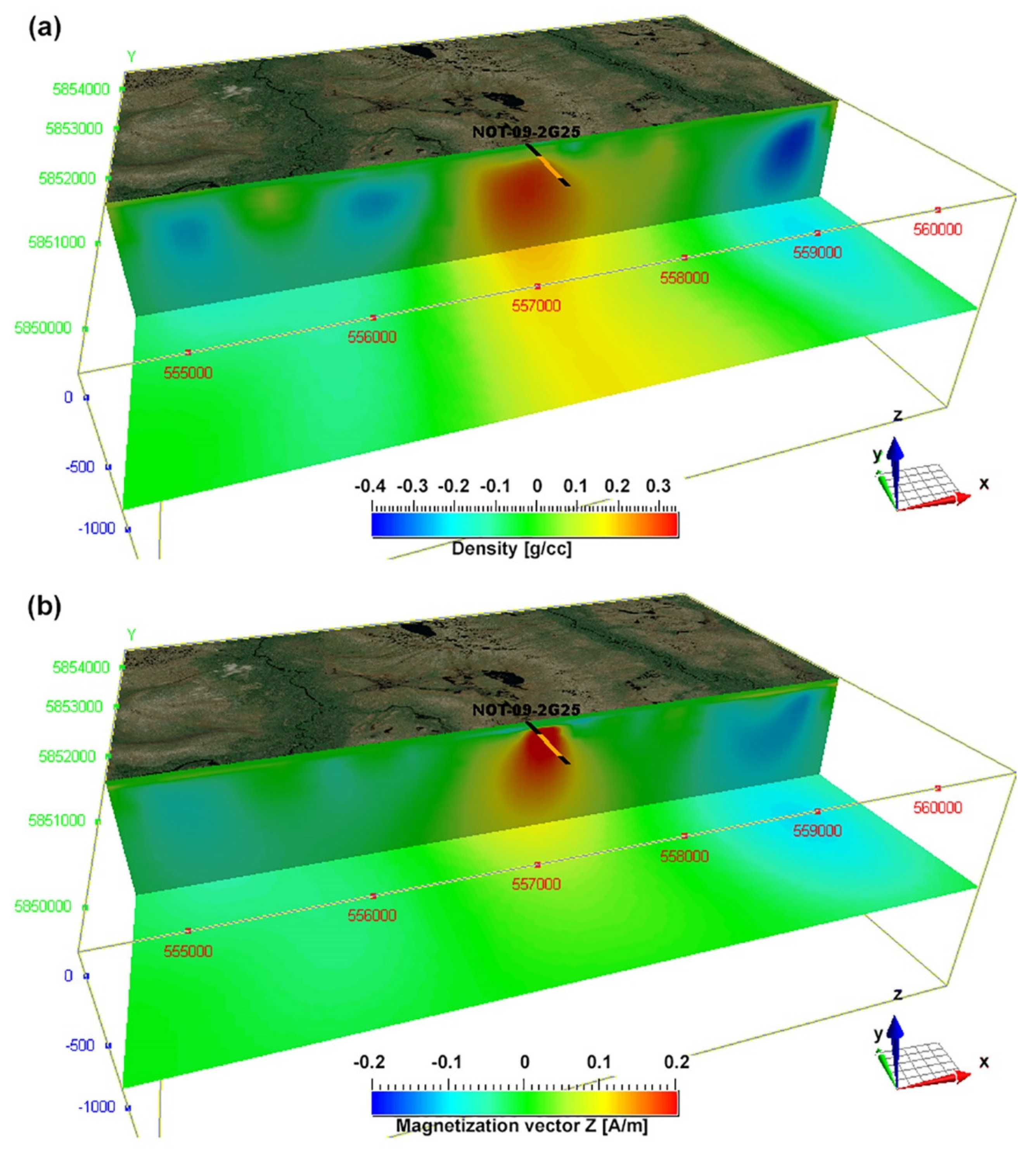
Finally,
Figure 12 presents a comparison of the inverse density (top panel) and vertical component of magnetization models (bottom panel) recovered by joint focusing inversion. It was shown in [
11] that it can be challenging to resolve a steeply dipping magnetic dike and recover a good data fit when inverting for magnetic susceptibility only. By inverting for the full magnetization vector, it is much easier to fit these structures and still retain a good data fit. Including these additional inversion parameters increases the non-uniqueness of the potential field inverse problem; however, we have remedied this with the addition of the Gramian and joint focusing constraints.
7. Conclusions
Magnetic data contain information about the remanent magnetization of rock formations that are often ignored when inverting for magnetic susceptibility only. We have introduced two novel methods of joint inversion of potential field data in the presence of remanent magnetization: (1) joint inversion subject to the Gramian constraint and (2) joint inversion subject to the joint focusing constraint. We have demonstrated the methods in a model study, and in a case study using airborne data acquired over the Thunderbird V-Ti-Fe deposit in the Ring of Fire area of Ontario, Canada. We have presented a comparison of the 3D models obtained using conventional single-datum standalone inversion and joint inversion subject to either the Gramian constraint or the joint focusing constraint. Comparison of the different inversion methodologies illustrates that 3D models obtained from joint inversion with either the Gramian or joint focusing constraint were able to resolve a shared earth model that featured sharper anomalous geospatial boundaries and a higher degree of structural correlation, as opposed to the 3D models obtained from standalone inversions. The joint inversion subject to the Gramian constraint did yield the highest degree of structural correlation; while the joint inversion subject to the joint focusing constraint provided comparable results but was much faster. By jointly inverting AGG and TMI data for density and magnetization vector, we demonstrated the efficiency of the novel methods in defining rock formations with remanent magnetization which are otherwise difficult to recover.
Author Contributions
Conceptualization, M.S.Z. and M.J.; methodology, M.S.Z.; software, M.J.; validation, M.J., and M.S.Z.; formal analysis, M.S.Z.; investigation, M.J.; resources, M.S.Z.; writing—original draft preparation, M.J.; writing—review and editing, M.S.Z.; visualization, M.J.; supervision, M.S.Z.; project administration, M.S.Z.; funding acquisition, M.S.Z. All authors have read and agreed to the published version of the manuscript.
Funding
This research was supported by Consortium for Electromagnetic Modeling and Inversion (CEMI), and TechnoImaging and received no external funding.
Data Availability Statement
The data used in this study are publicly available from the Ontario Geologic Survey.
Acknowledgments
The authors acknowledge the Consortium for Electromagnetic Modeling and Inversion (CEMI) at the University of Utah and TechnoImaging for the support of this research. The AGG and TMI data were collected by Fugro and made available by the Ontario Geological Survey, Canada.
Conflicts of Interest
The authors declare no conflict of interest.
References
- Jorgensen, M.; Zhdanov, M.S. 3D joint inversion of potential field data in the presence of remanent magnetization. In Expanded Abstracts, Proceedings of the 90th SEG International Exposition and Annual Meeting, Virtual Event, Houston, TX, USA, 11–16 October 2020; Society of Exploration Geophysicists: Tulsa, OK, USA, 2020; pp. 964–968. [Google Scholar]
- Lelièvre, P.G.; Oldenburg, D.W. A 3D total magnetization inversion applicable when significant, complicated remanence is present. Geophysics 2009, 74, L21–L30. [Google Scholar] [CrossRef]
- Li, Y.; Shearer, S.E.; Haney, M.M.; Dannemiller, N. Comprehensive approaches to 3D inversion of magnetic data affected by remanent magnetization. Geophysics 2010, 75, L1–L11. [Google Scholar] [CrossRef]
- Ellis, R.G.; De Wet, B.; Macleod, I.N. Inversion of magnetic data from remanent and induced sources. In Expanded Abstracts, Proceedings of the 22nd ASEG Geophysical Conference and Exhibition, Brisbane, Australia, 26–29 February 2012; ASEG: Crows Nest, Australia, 2012. [Google Scholar]
- Li, Y. From susceptibility to magnetization: Advances in the 3D inversion of magnetic data in the presence of significant remanent magnetization. In Proceedings of the Exploration 17: Sixth Decennial International Conference on Mineral Exploration, Toronto, ON, Canada, 22–25 October 2017; pp. 239–260. [Google Scholar]
- Zhu, Y.; Zhdanov, M.S.; Cuma, M. Inversion of TMI data for the magnetization vector using Gramian constraints. In Expanded Abstracts, Proceedings of the 85th SEG International Exposition and Annual Meeting, New Orleans, LA, USA, 18–23 October 2015; Society of Exploration Geophysicists: Tulsa, OK, USA, 2015; pp. 1602–1606. [Google Scholar]
- Zhdanov, M.S.; Gribenko, A.V.; Wilson, G. Generalized joint inversion of multimodal geophysical data using Gramian constraints. Geophys. Res. Lett. 2012, 39. [Google Scholar] [CrossRef]
- Gallardo, L.A.; Meju, M.A. Characterization of heterogeneous near-surface materials by joint 2D inversion of DC resistivity and seismic data. Geophys. Res. Lett. 2003, 30, 1658. [Google Scholar] [CrossRef]
- Zhdanov, M.S. Inverse Theory and Applications in Geophysics; Elsevier: Amsterdam, The Netherlands, 2015. [Google Scholar]
- Molodtsov, D.; Troyan, V. Multiphysics joint inversion through joint sparsity regularization. In Expanded Abstracts, Proceedings of the 88th SEG International Exposition and Annual Meeting, Houston, TX, USA, 29 September 2017; Society of Exploration Geophysicists: Tulsa, OK, USA, 2017; pp. 1262–1267. [Google Scholar]
- Zhdanov, M.S.; Cuma, M. Joint inversion of multimodal data using focusing stabilizers and Gramian constraints. In Expanded Abstracts, Proceedings of the 89th SEG International Exposition and Annual Meeting, Anaheim, CA, USA, 14–19 October 2018; Society of Exploration Geophysicists: Tulsa, OK, USA, 2018; pp. 1430–1434. [Google Scholar]
- Zhdanov, M.S. New advances in regularized inversion of gravity and electromagnetic data. Geophys. Prospect. 2009, 57, 463–478. [Google Scholar] [CrossRef]
- Li, Y.; Oldenburg, D.W. 3-D inversion of magnetic data. Geophysics 1996, 61, 394–408. [Google Scholar] [CrossRef]
- Li, Y.; Oldenburg, D.W. Fast inversion of large-scale magnetic data using wavelet transforms and a logarithmic barrier method. Geophys. J. Int. 2003, 152, 251–265. [Google Scholar] [CrossRef]
- Portniaguine, O.; Zhdanov, M.S. 3-D magnetic inversion with data compression and image focusing. Geophysics 2002, 67, 1532–1541. [Google Scholar] [CrossRef]
- Cuma, M.; Wilson, G.; Zhdanov, M.S. Large-scale 3D inversion of potential field data. Geophys. Prospect. 2012, 60, 1186–1199. [Google Scholar] [CrossRef]
- Zhdanov, M.S. Geophysical Inverse Theory and Regularization Problems; Elsevier: Amsterdam, The Netherlands, 2002. [Google Scholar]
- Molodtsov, D.M.; Troyan, V.N. Generalized multiparameter joint inversion using joint total variation: Application to MT, seismic and gravity data. In Expanded Abstracts, Proceedings of the 78th EAGE Conference & Exhibition—Workshops, Vienna, Austria, 29–30 May 2016; EAGE: Houten, The Netherlands, 2016. [Google Scholar]
- Zhdanov, M.S.; Tolstaya, E. Minimum support nonlinear parameterization in the solution of 3D magnetotelluric inverse problem. Inverse Probl. 2004, 20, 937–952. [Google Scholar] [CrossRef]
- Mungall, J.E.; Harvey, J.D.; Balch, S.J.; Azar, B.; Atkinson, J.; Hamilton, M.A. Eagle’s Nest: A magmatic Ni-Sulfide deposit in the James Bay Lowlands, Ontario, Canada. Soc. Econ. Geol. 2010, 15, 539–557. [Google Scholar]
- Ontario Geological Survey and Geological Survey of Canada. Ontario Geological Survey and Geological Survey of Canada. Ontario airborne geophysical surveys, gravity gradiometer and magnetic data, grid and profile data (ASCII and Geosoft formats) and vector data, McFaulds Lake area. In Ontario Geological Survey, Geophysical Data Set 1068; Ontario Geological Survey and Geological Survey of Canada: Sudbury, ON, Canada, 2011. [Google Scholar]
- Downey, M.; Atkinson, J. Report on Diamond Drill Program as Completed by Noront Resources Limited on Their Grid 2 Extension and Goodman Properties. Published Report. 2010. Available online: http://www.geologyontario.mndm.gov.on.ca (accessed on 23 May 2018).
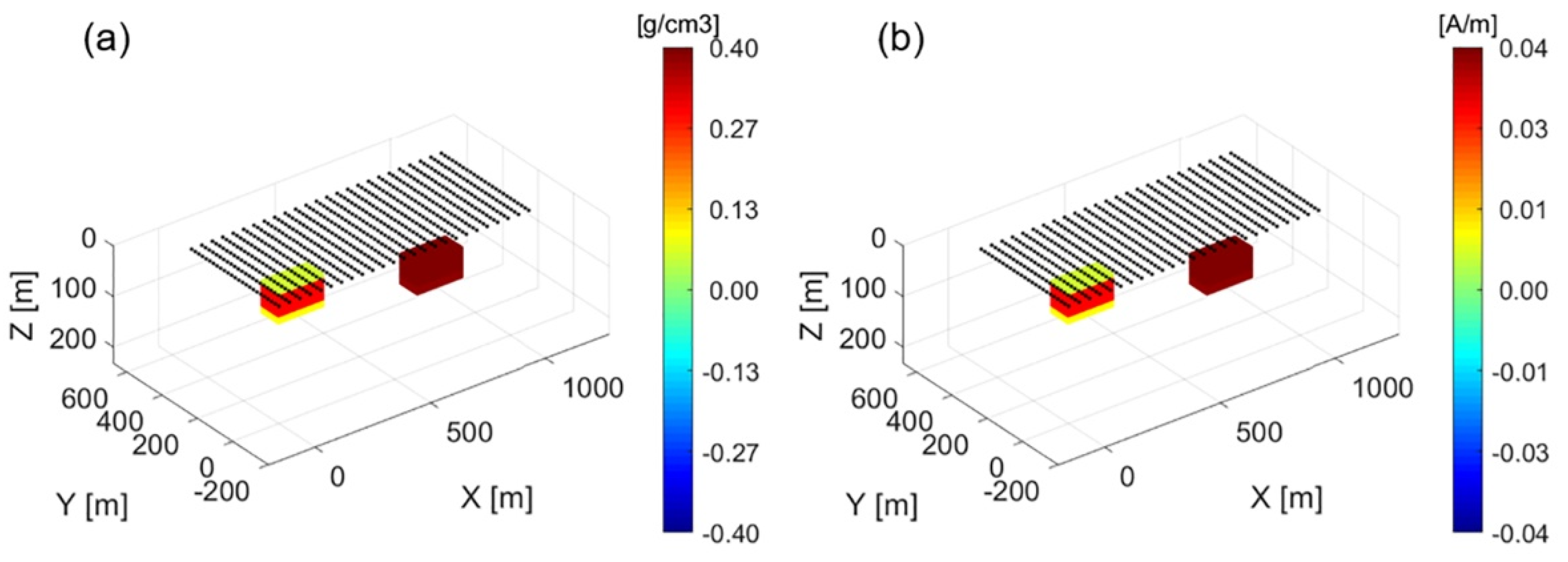
Figure 1.
Panels (a,b) show 3D views of the true density model and vertical component of magnetization vector model, respectively. The black dots represent the location of the observation stations.
Figure 1.
Panels (a,b) show 3D views of the true density model and vertical component of magnetization vector model, respectively. The black dots represent the location of the observation stations.
Figure 2.
Panels (a,b) show the true density model and magnetization vector model, respectively. Panels (c,d) show vertical sections of the density and magnetic vector models inverted standalone, respectively. Panels (e,f) show vertical sections of the density and magnetic vector models inverted with Gramian constraints, respectively. Panels (g,h) show vertical sections of the density and magnetic vector models inverted with joint focusing constraint, respectively. Panels (b,d,f,h) show the vertical component of the magnetic vector in color; the full magnetic vector is shown by black and white arrows, and the direction of the inducing field is shown by red arrows.
Figure 3.
Model study. Panels (a,b) show observed and predicted Gzz gravity gradient data inverted standalone, respectively. Panels (c,d) show observed and predicted total magnetic intensity (TMI) data inverted standalone, respectively. Panels (e,f) show observed and predicted Gzz gravity gradient data inverted with Gramian constraints, respectively. Panels (g,h) show observed and predicted TMI data inverted with Gramian constraints, respectively. Panels (i,j) show observed and predicted Gzz gravity gradient data inverted with joint focusing, respectively. Panels (k,l) show observed and predicted TMI data inverted with joint focusing, respectively.
Figure 4.
Geological map of the Ring of Fire area with marked known deposits (from [
20]).
Figure 4.
Geological map of the Ring of Fire area with marked known deposits (from [
20]).
Figure 5.
Airborne geophysical survey block in the McFaulds Lake region. airborne gravity gradiometry (AGG) and magnetic data were collected through the Fugro AGG and magnetic system (from [
21]).
Figure 5.
Airborne geophysical survey block in the McFaulds Lake region. airborne gravity gradiometry (AGG) and magnetic data were collected through the Fugro AGG and magnetic system (from [
21]).
Figure 6.
Panel (a) shows the Gzz component of the observed AGG data in UTM (16N) coordinates in panel (a). Panel (b) presents the filtered TMI data map with the removed regional trend. Profile AA’ is shown by the black line. The location of drill hole NOT-09-2G25 is shown by the black asterisk.
Figure 6.
Panel (a) shows the Gzz component of the observed AGG data in UTM (16N) coordinates in panel (a). Panel (b) presents the filtered TMI data map with the removed regional trend. Profile AA’ is shown by the black line. The location of drill hole NOT-09-2G25 is shown by the black asterisk.
Figure 7.
Panels (a,b) show vertical sections of the 3D density and magnetization vector models obtained from standalone inversions, respectively. Panels (c,d) show vertical sections of the 3D density and magnetization vector models obtained from joint inversion with Gramian constraints, respectively. Panels (e,f) show vertical sections of the 3D density and magnetizations vector models obtained from joint inversion with joint focusing constraint, respectively. Panels (b,d,f) show the vertical component of magnetization vector in color; the full magnetization vector is shown by the black arrows, and the inducing field direction is shown by the red arrows.
Figure 8.
Case study. Panels (a,b) show observed and predicted Gzz gravity gradient data inverted standalone, respectively. Panels (c,d) show observed and predicted TMI data inverted standalone, respectively. Panels (e,f) show observed and predicted Gzz gravity gradient data inverted jointly with Gramian constraints, respectively. Panels (g,h) show observed and predicted TMI data inverted jointly with Gramian constraints, respectively. Panels (i,j) show observed and predicted Gzz gravity gradient data inverted with joint focusing, respectively. Panels (k,l) show observed and predicted TMI data inverted with joint focusing, respectively.
Figure 9.
Model parameter cross plots shown in Panels (a–c) correspond to the standalone inversions, joint Gramian inversion, and joint focusing inversion, respectively.
Figure 9.
Model parameter cross plots shown in Panels (a–c) correspond to the standalone inversions, joint Gramian inversion, and joint focusing inversion, respectively.
Figure 10.
Left panel (a) shows the vertical section of the inverse model for susceptibility inversion. Right panel (b) shows a vertical section of the inverse model for magnetization vector inversion. The small black arrows in the right panel represent the magnetization vectors, while the color bar reflects the vertical component of magnetization.
Figure 11.
Comparison of 3D inverse models with drilling results. Left panel (a) shows the volume image of the inverse susceptibility model. Right panel (b) presents the volume image of the vertical component of the magnetization vector. The black–yellow–black solid line shows the location of the borehole drilled in the survey area. The yellow color indicates the mineralization zone confirmed by drilling.
Figure 12.
Top panel (a) shows the cut-off 3D image of the inverse density model. Bottom panel (b) presents the volume image of the vertical component of the magnetization vector. The black–yellow–black solid line shows the location of the borehole drilled in the survey area. The yellow color indicates the mineralization zone confirmed by drilling.
Table 1.
Correlation coefficient for different inversion scenarios.
Table 1.
Correlation coefficient for different inversion scenarios.
| Inversion Type | Correlation Coefficient |
|---|
| Standalone | 8.0 |
| Gramian | 8.9 |
| Joint focusing | 8.5 |
| Publisher’s Note: MDPI stays neutral with regard to jurisdictional claims in published maps and institutional affiliations. |
© 2021 by the authors. Licensee MDPI, Basel, Switzerland. This article is an open access article distributed under the terms and conditions of the Creative Commons Attribution (CC BY) license (https://creativecommons.org/licenses/by/4.0/).


