Investigation of Magneto-/Radio-Metric Behavior in Order to Identify an Estimator Model Using K-Means Clustering and Artificial Neural Network (ANN) (Iron Ore Deposit, Yazd, IRAN)

Abstract

The study area is located near Toot village in the Yazd province of Iran, which is considered in terms of its iron mineralization potential. In this area, due to radioactivity, radiometric surveys were performed in a part of the area where magnetometric studies have also been performed. According to geological studies, the presence of magnetic anomalies can have a complex relationship with the intensity of radioactivity of radioactive elements. Using the K-means clustering method, the centers of the clusters were calculated with and without considering the coordinates of radiometric points. Finally, the behavior of the two variables of magnetic field strength and radioactivity of radioactive elements relative to each other was studied, and a mathematical relationship was presented to analyze the behavior of these two variables relative to each other. On the other hand, the increasing and then decreasing behavior of the intensity of the Earth’s magnetic field relative to the intensity of radioactivity of radioactive elements shows that it is possible to generalize the results of magnetometric surveys to radiometry without radiometric re-sampling in this region and neighboring areas. For this purpose, using the general regression neural network and backpropagation neural network (BPNN) methods, radiometric data were estimated with very good accuracy. The general regression neural network (GRNN) method, with more precision in estimation, was used as a model for estimating the radiation intensity of radioactive elements in other neighboring areas.

1. Introduction

Due to the expansion of industry and the need for more and more raw minerals, the importance of mineral exploration is felt more than ever in today’s world. New methods in the statistical analysis of mineral data help identify better mineral reserves, including geostatistical methods and methods based on artificial intelligence and machine learning [1,2,3,4]. Using advanced and intelligent methods, the accuracy of our performance in the field of mineral identification and exploration increases. Today, due to the advancement of technology and the rising level of technical knowledge, secondary mines have also been raised [2]. Secondary mines have been mined in the past with a higher threshold grade, and humans can today process low-grade minerals in them with the help of advanced technology [5,6,7].

Each of the methods used in statistical studies has special strengths and applications. However, these methods may have weaknesses and limitations [8,9]. One of the applied techniques in mineral data analysis (due to the large volume and data dimensions) is the clustering method [10]. The clustering technique is used to classify data. Accordingly, it has its applications in each branch of science. The application of clustering methods (e.g., K-means and hierarchical methods) is performed to analyze exploratory data, such as geochemistry and geophysics, to categorize data to achieve a specific goal [11,12]. One of the applications of the clustering method is in the analysis of geochemical data from the sampling of stream sediments. In this case, it is usually used to study the geochemical behavior of the elements and classify their concentration data [13,14]. The clustering technique can also be used in remote sensing (satellite image analysis) to identify alterations and lithology based on the wavelengths of satellite imagery bands [15,16].

The function of clustering analysis is to place data with similar characteristics in a specific group. Therefore, after applying clustering analysis to the data, instead of dealing with a large amount of data, we are faced with a series whose members are very similar in terms of features [17]. The purpose of using clustering analysis is to present the classes whose members are most similar to each other and more different from the members of other classes [18,19]. Existing behaviors can be identified based on the similarities that each member of a class has with each other. Identifying the behavior of the data (the behavior of each class relative to each other) is a great help in analyzing earth-related sciences [20]. The clustering technique is one of the indirect analytical methods. This means that, in using this method, there is no need to have information about the internal structures of the members, and, in fact, by using clustering, the hidden patterns in the data are identified. Using the results of this method, the process of direct studies can be improved [21,22].

One of the important and practical analytical methods in clustering is the K-means method. This method classifies data based on the Euclidean distance. The distance of each datum from the center of the cluster should be as small as possible. To achieve this goal, start with a small number of classes and increase the number of classes as much as possible. As a result, after plotting the cluster utility function, the appropriate number of clusters are identified, and clustering is performed based on that [23].

The K-means clustering analysis technique is used to study the behavior of the data relative to each other. Among the applications of this method that other researchers to date have performed is the study of the impact of vegetation on the process of restoring water health, the geological classification of land [17,24], the identification of geochemical patterns and geochemical behavior of elements in mineral studies [13], and predicting the amount of carbon in intelligent systems, as well as greenhouse gas emissions and their impact on the urban environment [21,22].

In recent decades, the use of methods based on artificial intelligence, including artificial neural networks (ANNs), has become particularly important. Artificial neural networks are programmed based on the processing capabilities of the human brain, including knowledge, control, speech, and prediction. Managing large volumes of data with complex relationships and many patterns, reasoning on ambiguous data, and providing fast and adequate responses are some of the capabilities of artificial neural networks (ANNs) [25,26,27]. In this study, by performing a string of codes in MATLAB software and using SPSS software, the capabilities of the mentioned methods were investigated. Based on the obtained results, it is possible to introduce a process to improve exploration operations in this area and reduce the costs of geophysical operations in neighboring areas.

In traditional geophysical iron exploration methods, magnetometric and radiometric data had to be collected directly in all parts of the region to identify mineral anomalies [28,29,30]. Collecting magnetometric and radiometric data directly requires a lot of time and cost [31]. In addition, in many projects, in order to plan the continuation of exploration operations, it is necessary to analyze the available data and provide an overview of the mining region. So, there is a need for a high accuracy estimator. This estimator should be able to estimate magnetometric and radiometric data based on each other, using surveys performed in the area. In this study, the other data can be predicted with high accuracy by combining the K-means clustering method and the artificial neural network (ANN) based on the behavior of the available data (magnetometry or radiometry). In this method, similar to what was done in the past to create a pseudo-gravity information layer based on magnetic data, the goal is to estimate each of the magnetometric and radiometric data based on each other [32]. The K-means clustering method was used to investigate and observe the behavior of magnetometric and radiometric data. The artificial neural network was then used to create an estimator model based on magnetometric data for radiometric estimation. The main advantage of the combined method based on K-means clustering and ANN is the possibility of estimating data based on each other with high validity in this method without the need for the simultaneous measuring of magnetometric and radiometric data. In this way, in addition to saving time, financial costs are also significantly reduced. Since the combination of the two methods has not been used before in estimating magnetometric and radiometric data, this study investigated the efficiency of this combined method.

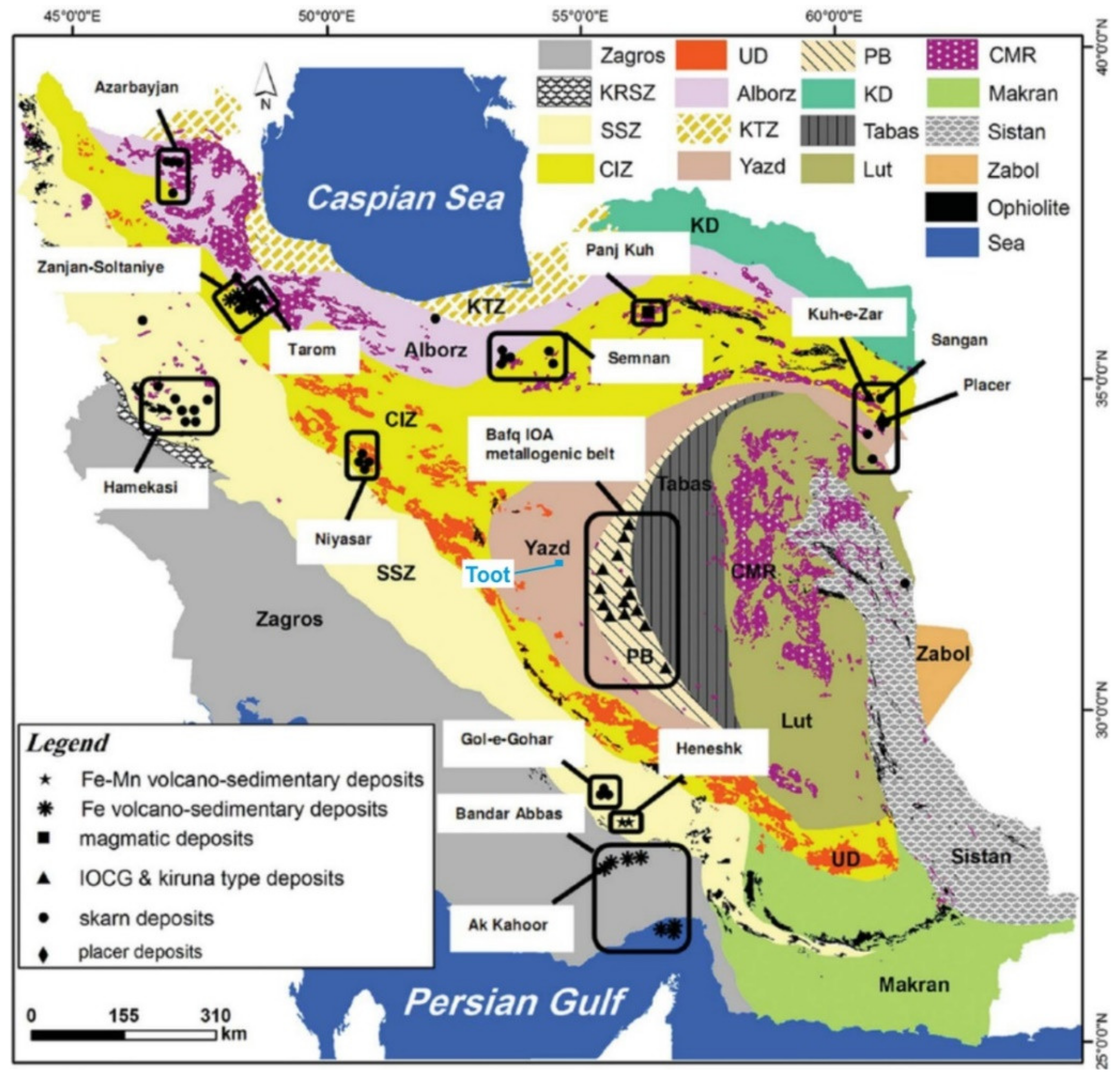
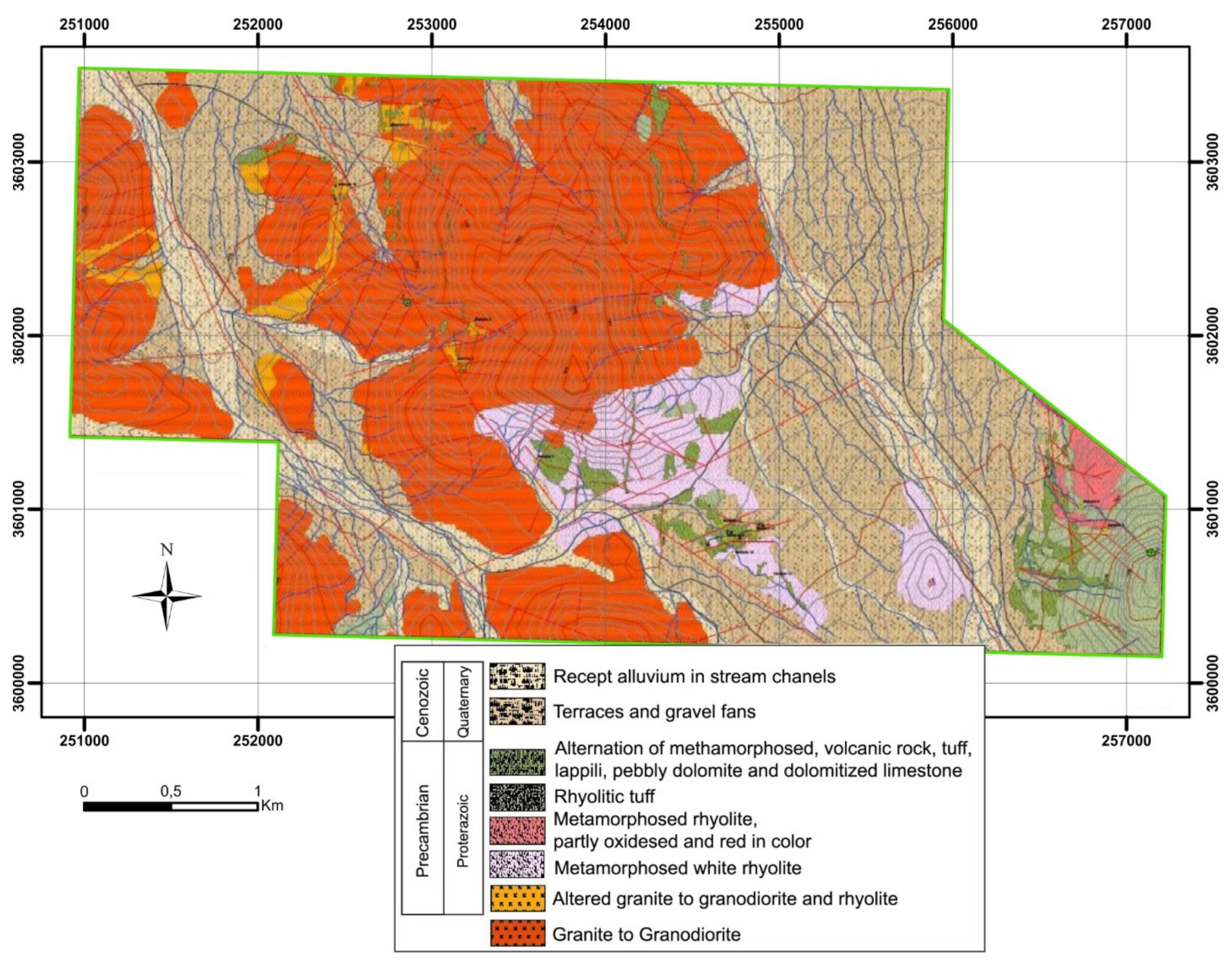
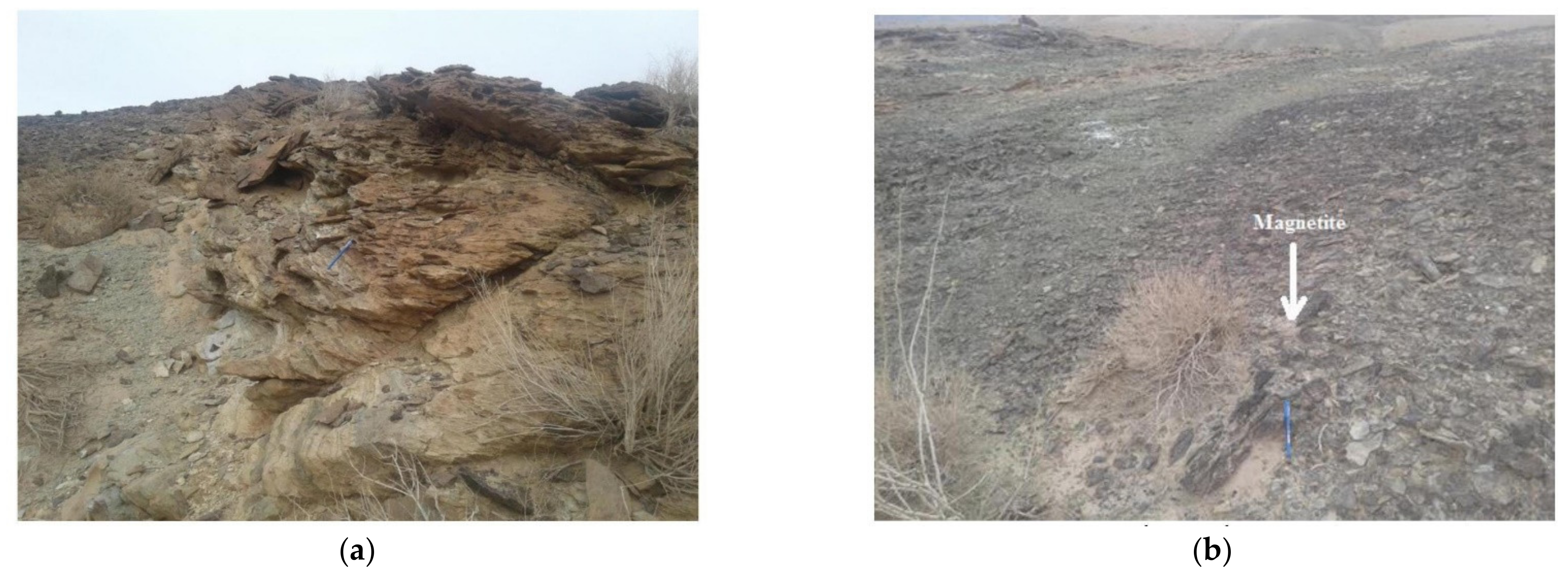
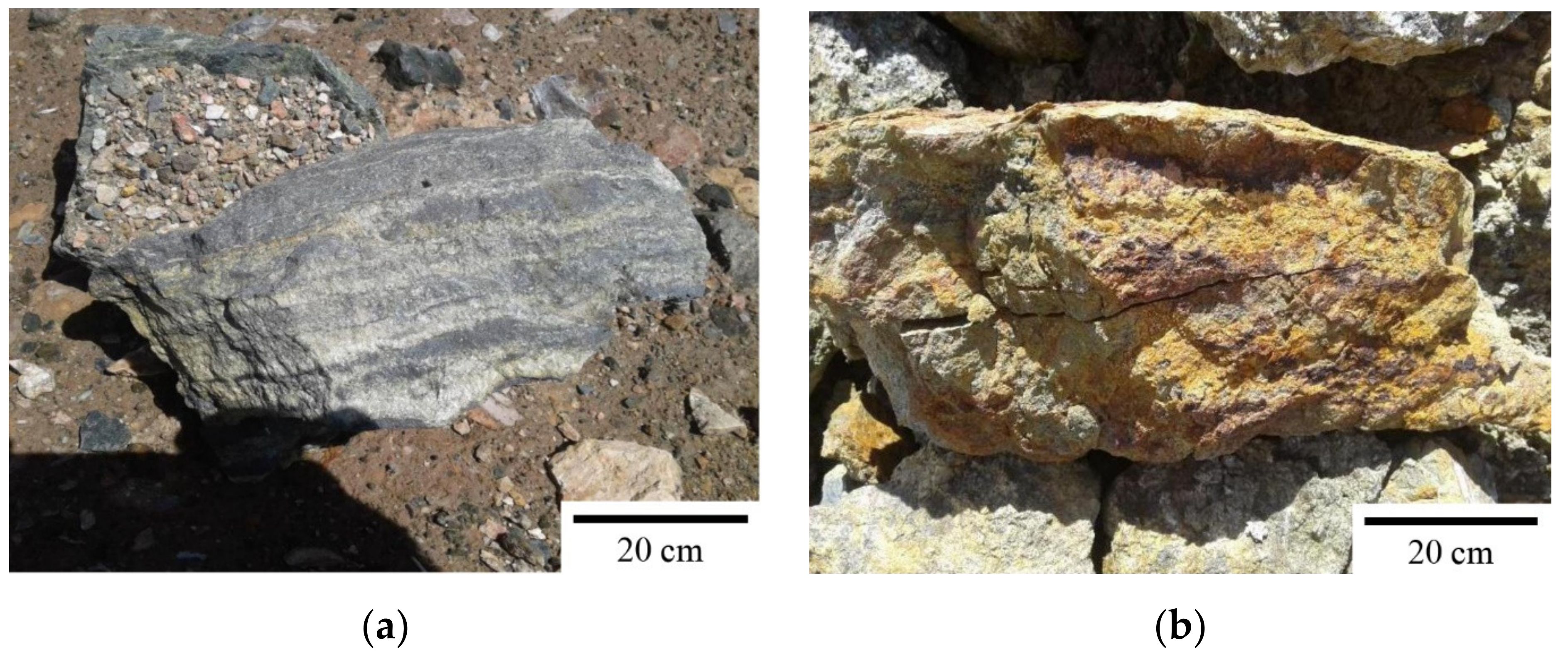
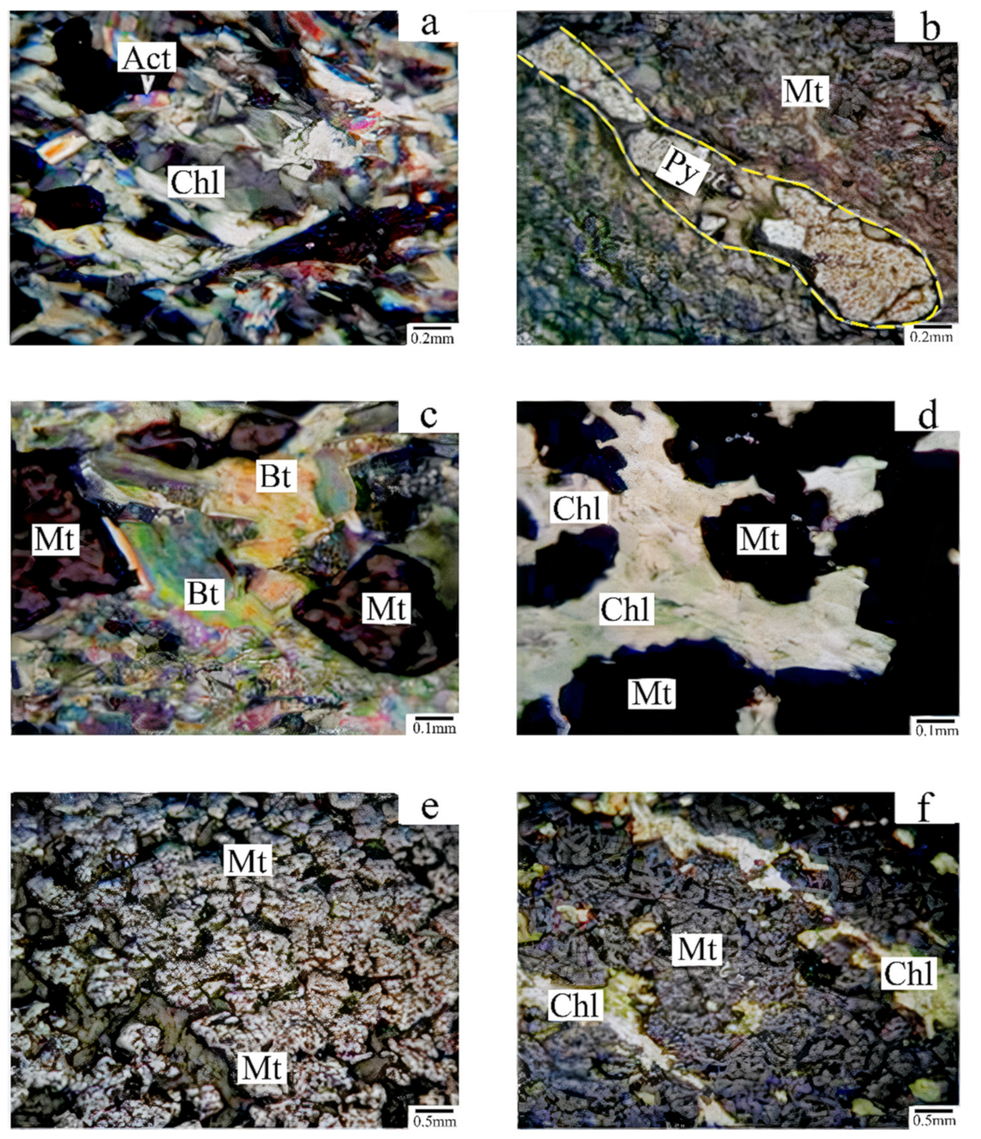
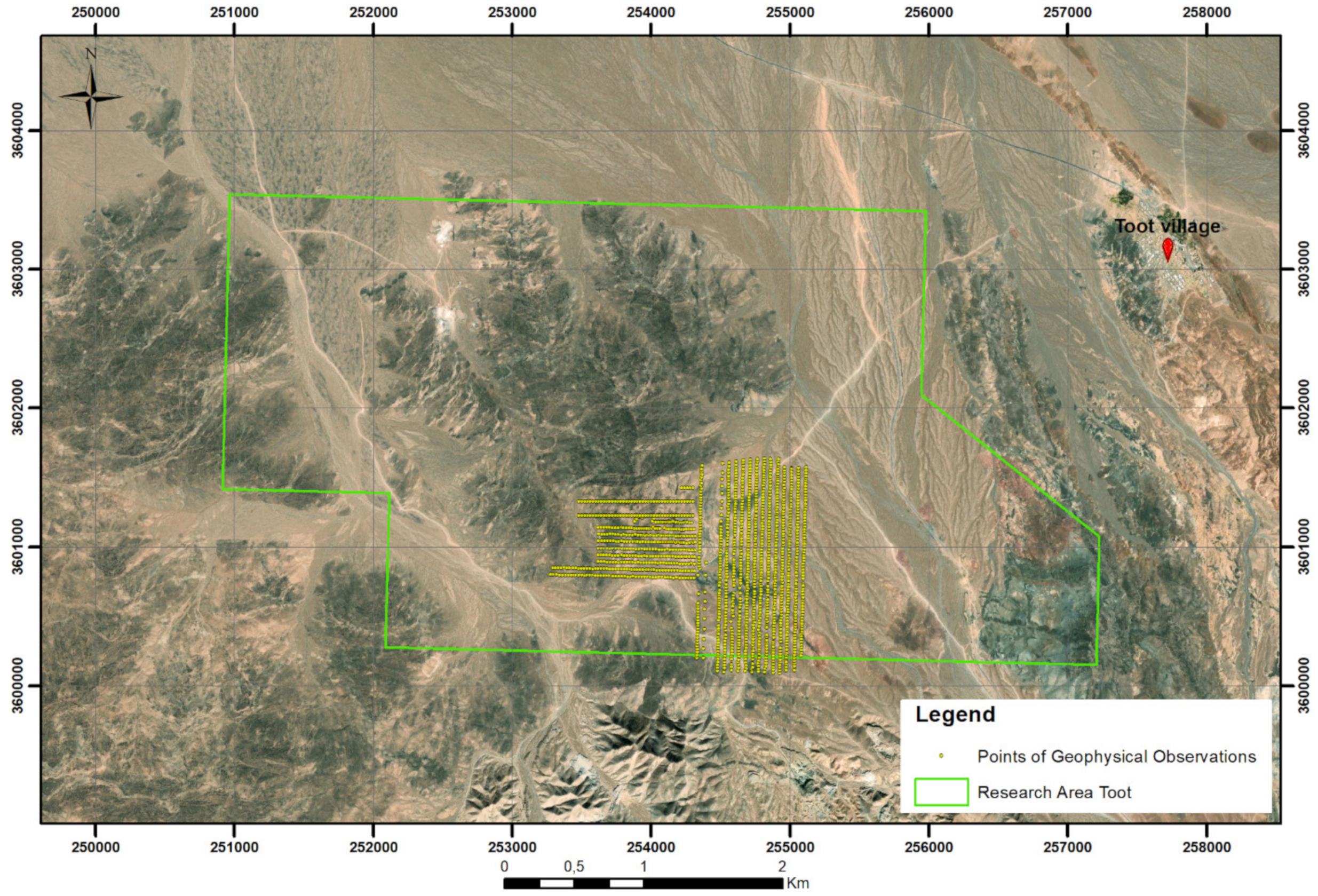
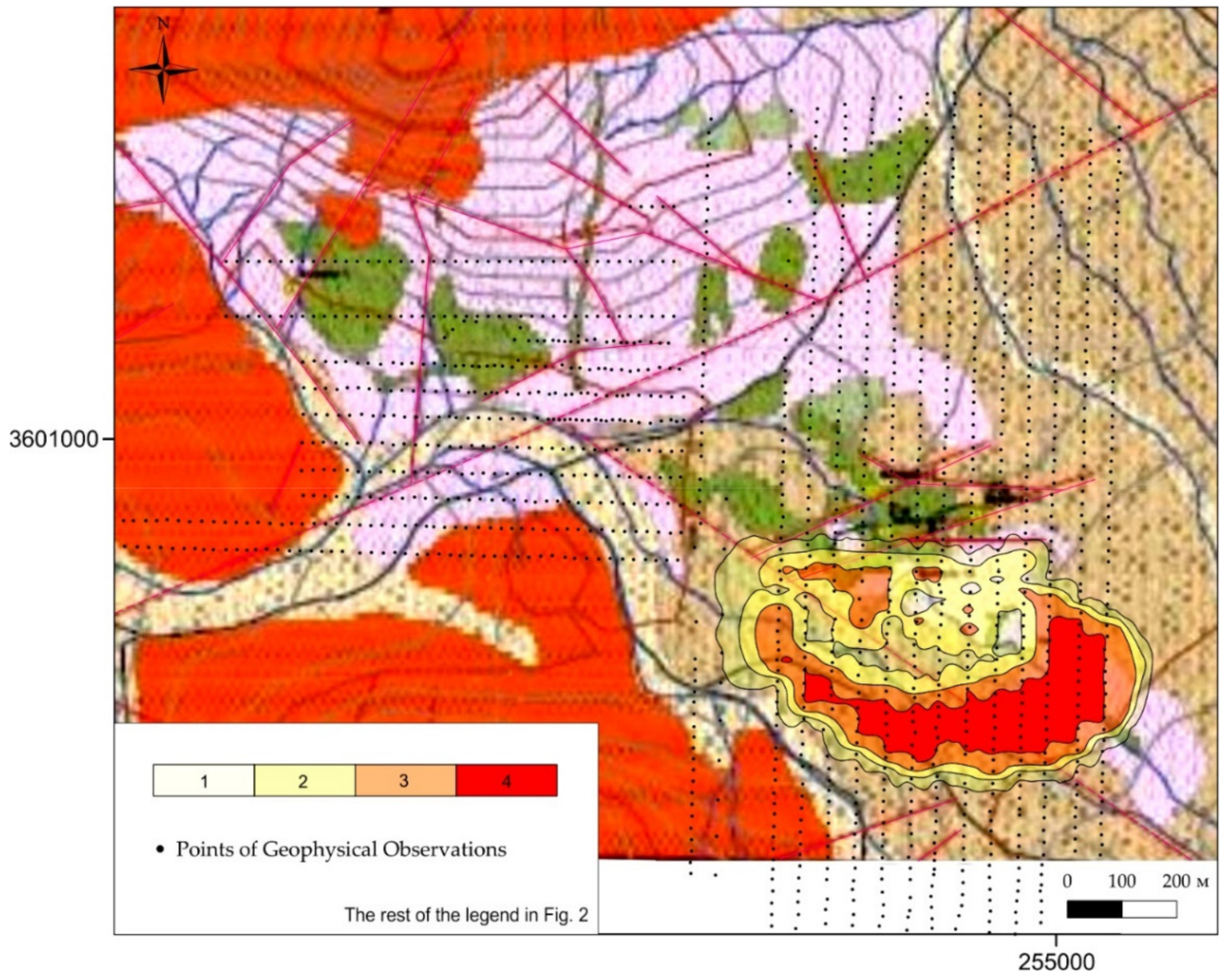
2. Geological Setting of the Studied Area

Iran is known as an oil country, but there are a variety of minerals and geotourism attractions in this country [33,34]. The Toot iron deposit is located in the structural zone of Central Iran and contains iron and possibly other metallic minerals (Figure 1).

The study area is located 5 km west of Toot and Anjiravand villages, to the northeast of Ardakan city in Yazd province [35]. The access road to the deposit is accessed from the Yazd–Choopanan road. The average height of the Toot deposit is about 1337 m above sea level.

The study area is located 5 km west of Toot and Anjiravand villages, to the northeast of Ardakan city in Yazd province [36]. The access road to the deposit is accessed from the Yazd–Choopanan road. The average height of the Toot deposit is about 1337 m above sea level.

In terms of geological structural divisions, the study area is located in the west of the Central Iran zone, Yazd block and the west of the Ardakan geological area (at the scale 1:250,000), and the southeast of the Mehdiabad geological area (at the scale 1:100,000). Around this area, low-metamorphic volcanic, intrusive, and sedimentary rocks are exposed, the age of which, due to their physical resemblance to the Rizo series, has been attributed to the Infracambrian. Still, micro-paleontological evidence indicates that these sedimentary and volcanic series are from the Lower Ordovician era. The study area consists of granite, white rhyolite, Cretaceous sediments, and alluvial sediments of the present era. The most important tectonic elements are faults, and the tectonic structure of the area has been formed under the influence of strike-slip faults. Different rocks have been deformed due to these tectonic forces, and different microstructures have been formed in them. The faults that have the most important role in the Toot area have a northwest–southeast trend and, together with sub-faults, control the mineralization in the area. These faults have played an essential role in the formation of metallic and non-metallic mineralization. The following figure shows the trend of major and minor faults in the Toot area. Figure 2 shows the geological map of the area [37,38].

Iron mineralization is located in the southern part of the study area, where metamorphic schist rocks host iron ores, with carbonate rocks including dolomite and dolomite limestone also found in the form of thin, lenticular layers. The existing schists have been formed as regional metamorphisms in the greenschist facies, and their possible protolith could be basaltic igneous rocks (Figure 3). In this area, due to erosion and soil formation processes, anomalies of host rock outcrops and mineral outcrops are reduced, and iron mineralization in the ground can be seen in the form of small protrusions (up to several square meters).

Based on initial fieldwork, there are various indices of iron mineralization in and around the target areas, which are visible mainly in the form of a mass, streak, and scatter. Banded mineralization involves the alternation of high-grade magnetite-rich and low-grade quartz-rich laminates. Due to weathering in the superficial parts of the anomaly, magnetite is replaced by hematite and limonite (Figure 4).

Meanwhile, studies of the cross-sections of thin and polished cross-sections show that its metal ores are mainly magnetite and pyrite, and its non-metallic ores are chlorite, actinolite, mica and carbonate minerals (Figure 5a,b). The most important magnetic tissue visible in the specimens is the scattered grain-to-mass tissue, which contains scattered magnetite crystals in a field of tailing minerals (Figure 5c–f). The presence of these crystals in magnetite depends on its origin. Their inclusion in the ore can indicate the existence of a regenerative environment after mineralization and the presence of sulfur from one or more possible sources. Samples taken from deep areas demonstrate a small number of these stains surrounding pyrite. Still, most of these stains are scattered in the cross-section of the samples without any connection to pyrite and magnetite minerals. Malachite mineralization is also rarely observed in scattered anomalous surfaces and oxide sections.

The textural evidence suggests that pyrite and magnetite minerals were present in the igneous protolith before the metamorphic event, which underwent recrystallization due to the metamorphism, or that the mineralization event was associated with the activation of mineralizing fluids and thermal solutions during the transformation event. Considering the phenomenon of arterial silicification in rocks of an anomalous range, which indicates the entry of silica with hydrothermal solutions into fractures and sedimentation within them, the theory of the relationship between the mineralization event and the activation of mineralization fluids during a metamorphic event can be considered more probable.

3. Methodology and Materials

3.1. Raw Data

In the study area, data from 1439 magnetometric and radiometric points were collected in similar situations. Figure 6 shows the position of the study area on a satellite image.

To estimate the radioactive intensity of radioactive elements in the region and investigate their behavior relative to the intensity of the Earth’s magnetic field, the values of their correlation coefficients were studied and processed. As Spearman correlation coefficients, the correlation coefficient value is 0/077 [39,40] that of these two data are weak and indicate a strong lack of correlation between them. Additionally, in Figure 7, the histogram of magnetometric and radiometric data can be seen simultaneously. This histogram shows that the two data sets are normal and can be easily clustered. It can also be seen that the spread of radiometric data is greater than magnetometric data, and it is better to standardize them before applying the methods. The data type of magnetometric is Nano Tesla and Gamma, which belongs to radiometric data is Becquerel per kilogram.

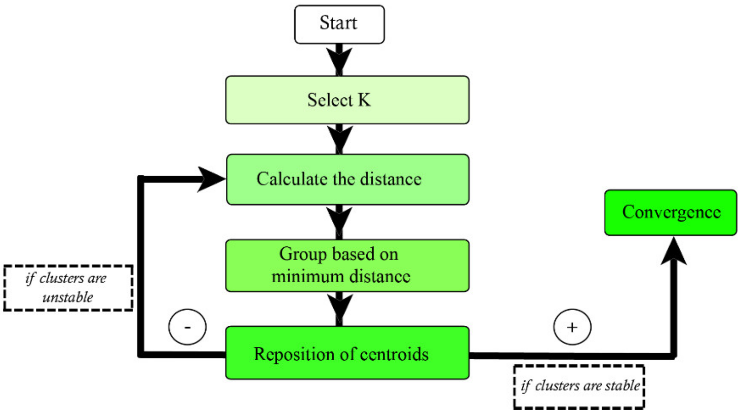
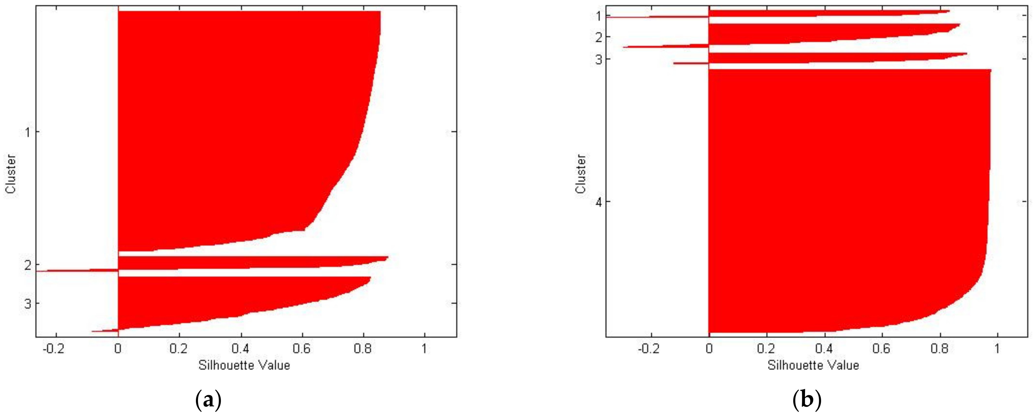
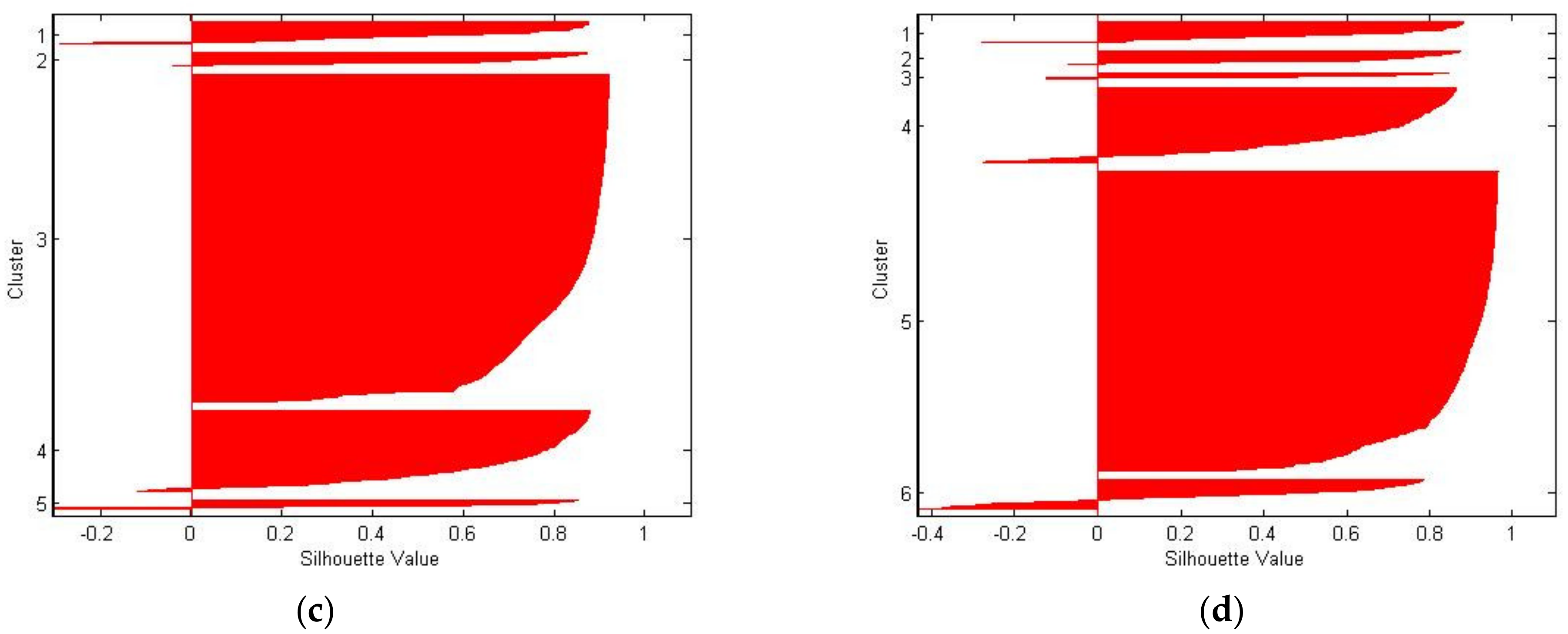
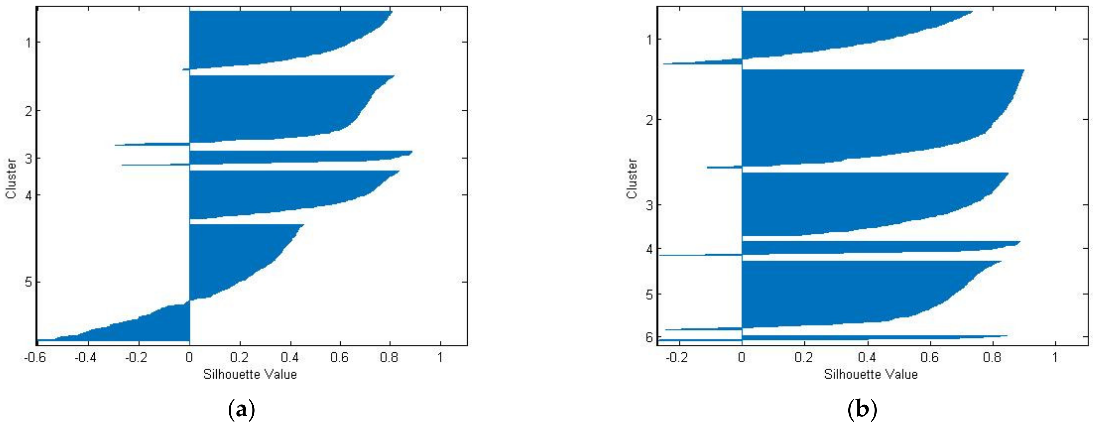
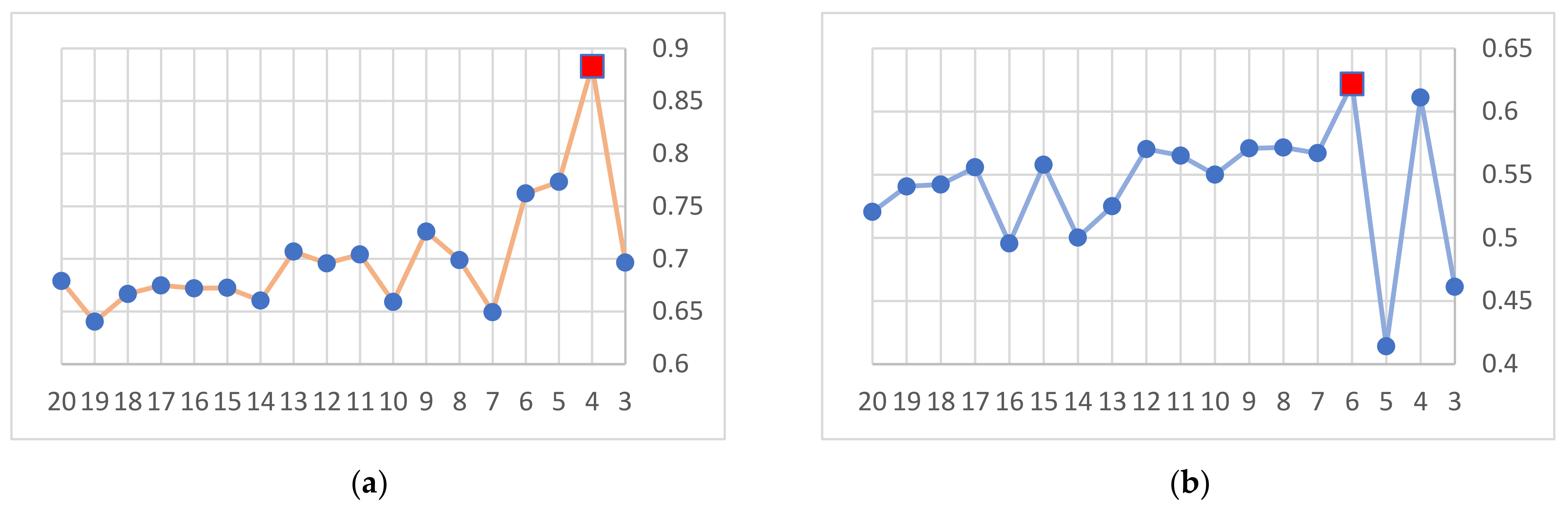
3.2. K-Means Clustering Method

The K-means clustering method, in order to cluster the data, starts its process by considering the number of (k) classes. The goal of the algorithm is to find the optimal number of clusters whose members have the shortest distance from the center of the cluster [41]. The K-means clustering analysis technique initially considers a number of batch centers randomly from among the data. It then tries to collect other data based on the shortest Euclidean distance around these cluster centers, and thus clusters are obtained. This algorithm is repeated until the optimal cluster centers are determined [42,43,44].

The procedure steps of the K-means clustering algorithm are [45]:

1. n members are divided among K clusters.

2. To calculate the center of each cluster, the vector Zj is calculated according to Formula (1).

$${\mathrm{z}}_{\mathrm{j}}=\frac{{{\displaystyle \sum }}_{\mathrm{x}\in {\mathrm{c}}_{\mathrm{j}}}\mathrm{x}}{\#{\mathrm{c}}_{\mathrm{j}}}\mathrm{for}\mathrm{j}=1.\dots .\mathrm{k}.$$

(1)

3. In Formula (1), x is the vector corresponding to each member belonging to the cluster of Cj, and #Cj is the number of members in the cluster of Cj. Formula (2) is used to calculate the center of each cluster while running the algorithm [45].

4. Calculate the objective function based on Formula (2), which calculates the distance of members from the center of the cluster.

$$f\left(C_1.C_2.\cdots .C_k\right)={{\displaystyle \sum }}_{j-1}^k{{\displaystyle \sum }}_{X\in C_j}{\left|X-z_j\right|}^2.$$

(2)

5. The objective function of Formula (2) is minimized, and the appropriate clustering with K clusters is identified. In general, the use of programming and computer speeds up the performance of the above algorithm [46,47].

The K-means clustering algorithm is schematically presented in Figure 8.

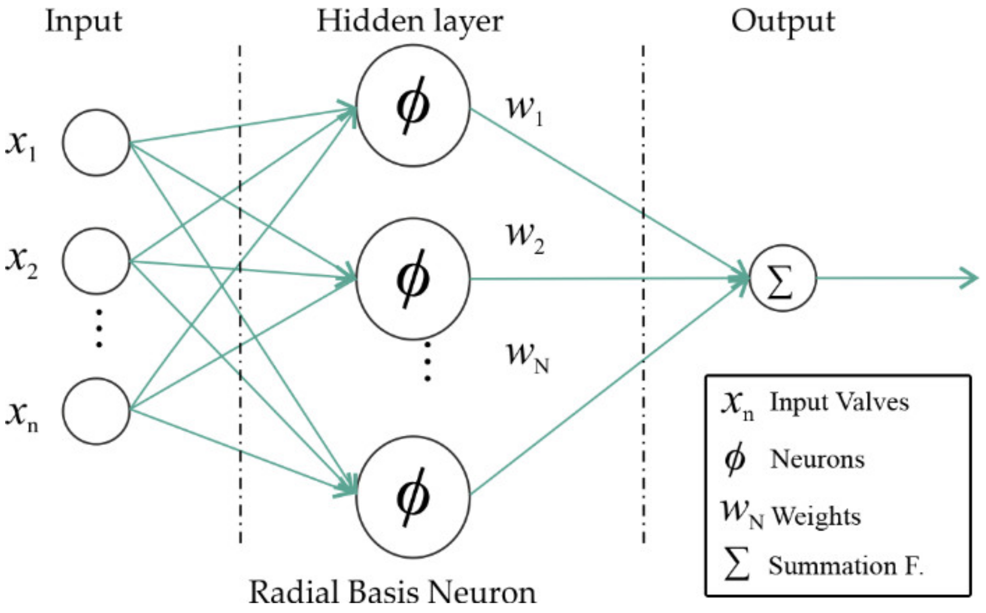
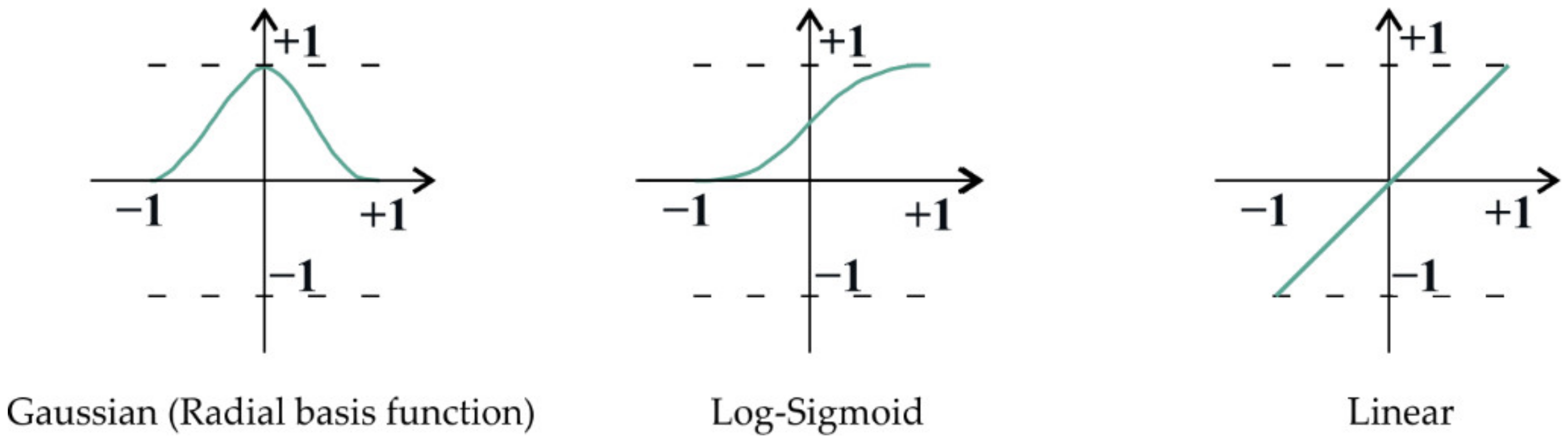
3.3. Artificial Neural Network (ANN)

According to many scientists, the human brain is the most complex system ever observed and studied throughout the universe. However, this complex system does not have galaxy-sized dimensions and no more components than today’s supercomputer processors. The general structure of the artificial neural network (ANN) is shown in Figure 9.

In this study, two types of linear and sigmoid activating functions were used. These choices are the standardization of data in preprocessing, nonlinear increase of data, and then linearization of results. This combination of functions is suitable for this study due to gradual changes. More precisely, activator functions decide whether or not a particular neuron is activated in neural networks, so, the correct choice of activator functions can increase network accuracy and prevent over-fitting.

A simple, albeit slightly inaccurate, the definition of activator functions are parts of neural networks whose input is a number (small or large at an arbitrary interval) and whose output is usually between 0 and 1, or −1 and +1. These functions convert an input number to a specific interval (for example, −1 to +1). Activator functions are also called transfer functions (Figure 10) [48,49].

The outputs match the desired outputs as closely as possible. According to the learning algorithm, several types of neural network, such as the backpropagation neural network (BPNN), the probabilistic neural network (PNN), and the general regression neural network (GRNN), have been designed in MATLAB software. The GRNN and BPNN methods were used in this study [50].

4. Results and Discussion

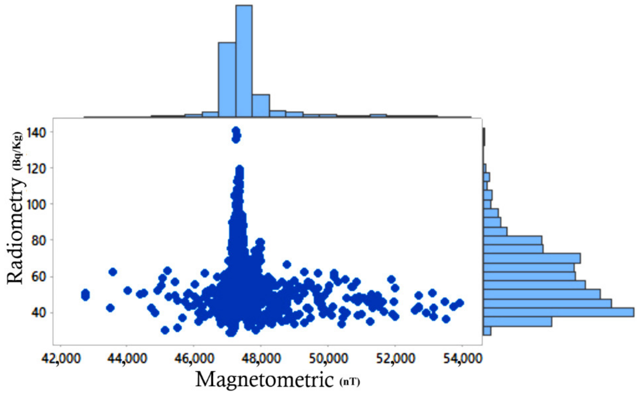
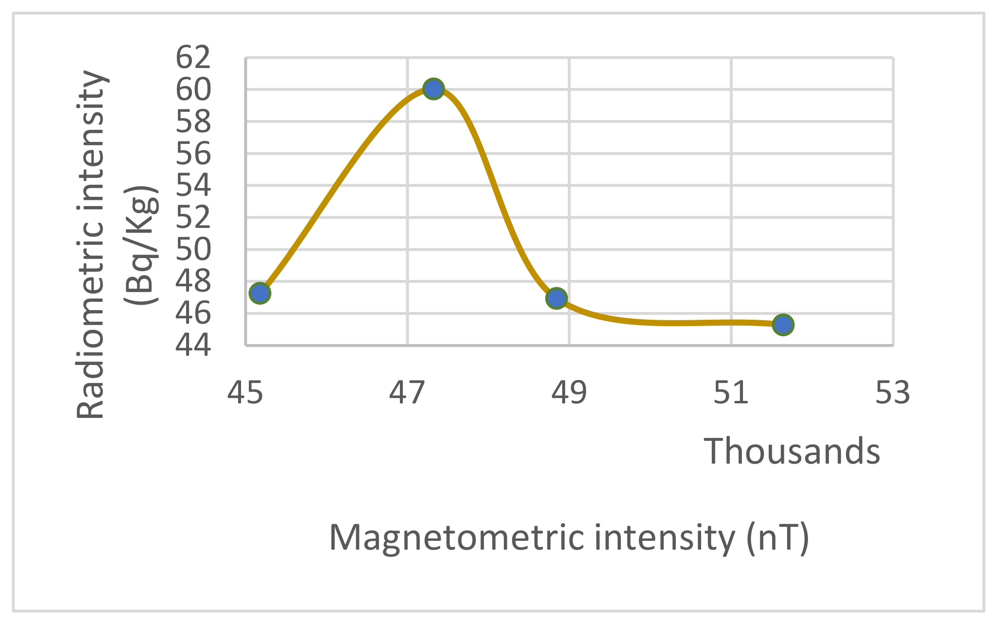
4.1. Behavior Study of Radiometry and Magnetometry Surveys

In order to investigate the behavior of magnetometric and radiometric data relative to each other in the region, the K-means clustering analysis algorithm was used.

The number of clusters from K = 3 to K = 20 was considered, and the amount of utility function was calculated for each of the clusters performed. K-means clustering analysis was performed on magnetometric and radiometric data once with the geographical coordinates of the sample and again without considering the geographical coordinates. Then, according to the profiles (S (i)) obtained from the data classification and the graph of the utility function values, optimal clustering should be selected.

The mean value of the utility function in clustering performed on uncoordinated data is 0.8830 (as shown in Figure 11). This value is the highest utility function value among the clusters formed; the number k was increased to 100 to ensure that the desired result was found. The results of this measure show that the utility function decreases significantly after clustering with k = 20. Figure 12 shows the profiles drawn from the clustering of radiometric and magnetometric data with coordinates. Based on the mean values of the utility function, six-class clustering with a value of 0.6220 is optimal.

The graph of the mean value of the utility function versus the number of clusters is shown in Figure 13. Based on the results of magnetometric and radiometric data clustering, which was performed once with coordinates and again without coordinates, the optimal clustering should be selected. As shown in Figure 13, clustering data without coordinates have the highest value of the function in four-class clustering. Therefore, this clustering was selected as the optimal clustering.

Additionally, according to the quality function and p (k) value, the appropriate number of clusters is determined. To determine the number of clusters, the value of p (k) is calculated using Equation (3) for different values of k.

$$\rho \left(k\right)=\frac{1}{k}{{\displaystyle \sum }}_{n=1}^k\left(m_{i}n\left\{\frac{{\eta }_n+{\eta }_m}{{\delta }_{nm}}\right\}\right).$$

(3)

As mentioned, the maximum value of p (k) indicates the appropriate number of clusters.

Table 1. Values p (k) for the number of different clusters.

p(k)	Number of Clusters	Parameters
6937/0	3	Measurements without Location
7898/0	4
6998/0	5
4845/0	6
5046/0	7
2774/0	8
4490/0	9
5452/0	10
2042/0	3	Measurements with Location
2321/0	4
3701/0	5
5775/0	6
3767/0	7
4843/0	8
2116/0	9
3176/0	10

Note. Maximum value (p) in red.

shows the values of p (k) obtained corresponding to the number of clusters. In the behavior study of two parameters without coordinates, 0.7898 is the maximum value. So, the most appropriate number of clusters is equal to four, and similarly, for combinations with coordinates, the most appropriate number of clusters is equal to six. As can be seen, the number of suitable clusters obtained from the quality function corresponds to the results of the criterion S (i).

The centers of the designated categories for the best classification are shown in Figure 14 for data without locations for four classes.

According to this classification, shown in Figure 15, to increase the intensity of the magnetic field, the intensity of the radiation first increases. After increasing the intensity of the magnetic field to 47,500 nT, it follows a decreasing trend. A magnetic field intensity of 49,000 nT does not cause unusual behavior in the region. Due to these increases and decreases, the best third-degree curve has negative concavity. The equation of the fitting lines can be expressed as:

$$\mathsf{\gamma }=9{\mathrm{E}}^{-10}{\left(\mathrm{nT}\right)}^3-0.0001{\left(\mathrm{nT}\right)}^2+6.3787{\left(\mathrm{nT}\right)}^1-102935$$

(4)

and its correlation coefficient is equal to R² = 0.95.

According to the four divided classes, the separated classes are shown in Figure 14. At a magnetic intensity of 49,000 nT, the rocks in the region reach radioactive stability of 45 gamma. This result indicates that radiometric changes based on magnetometric data occurred only in the range of 45,000 to 49,000 nT in the study area. The highest gamma intensity in the region occurred at a magnetic intensity of 47,500 nT. Therefore, the anomalous areas identified based on class 2 have the highest amount of radioactivity.

The details of each of the cluster centers are presented in

Table 2. Cluster center specifications.

X	Y	Radiometry (Bq/Kg)	Magnetometry (nT)	Cluster
253952.7	3601024	74	47,356	First
254764.3	3600361	50	47,998	Second
254789.2	3601391	54	47,230	Third
254797.9	3600956	45	46,953	Fourth
254649.8	3600745	48	44,865	Fifth
254783.6	3600612	46	51,147	Sixth

.

4.2. Radiometric Measurements Prediction

In this section, the methods of GRNN and BPNN in MATLAB software were used. We determine the ability to estimate radiometric data by means of magnetometric surveys based on the length and width. Using 70% of the randomly selected data and determining the estimate’s validity with the remaining 30% data. For better estimation, the values in the range of zero to one are standardized according to Equation (5) [51].

$$X_{norm}=\frac{X-X_{min}}{X_{max}-X_{min}}$$

(5)

Radiometric measurement values are introduced as output variables, and magnetometric harvest values, along with the length and width of points, are introduced as input variables to determine the estimation algorithm.

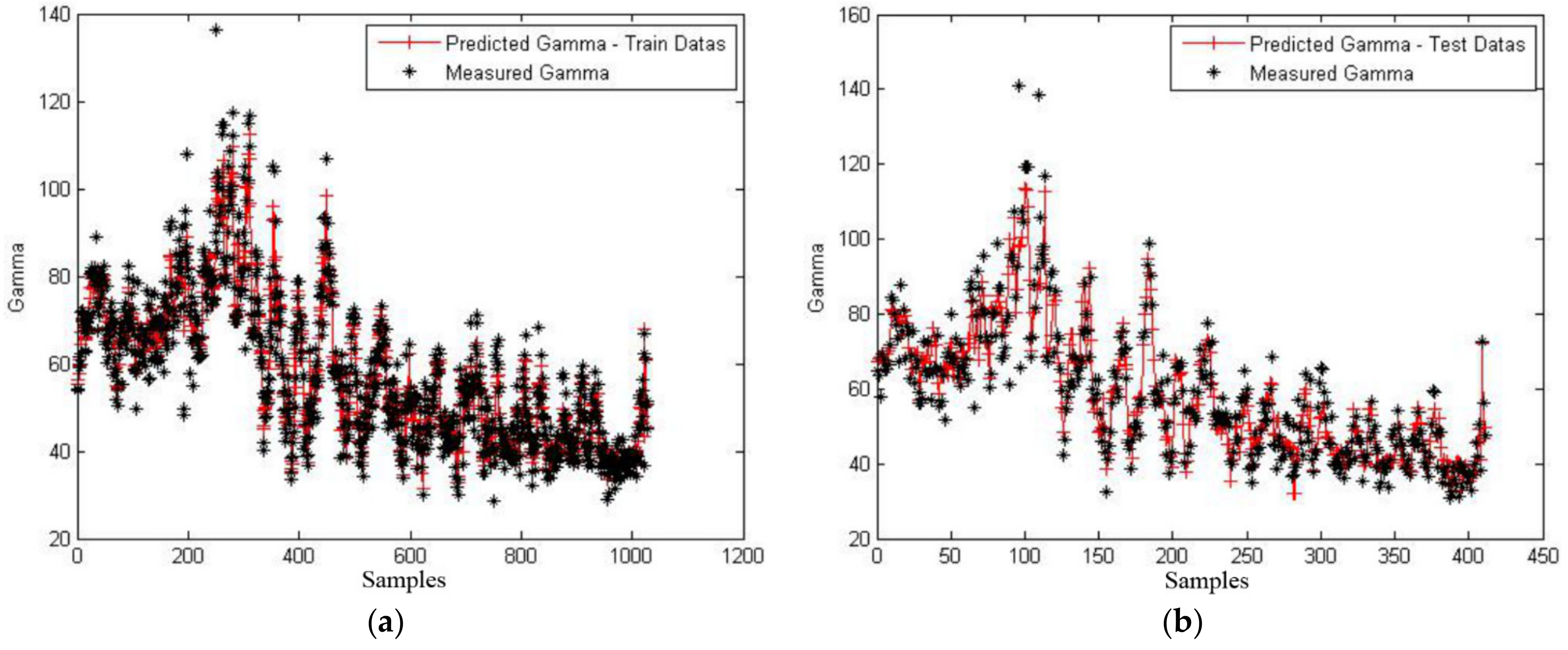
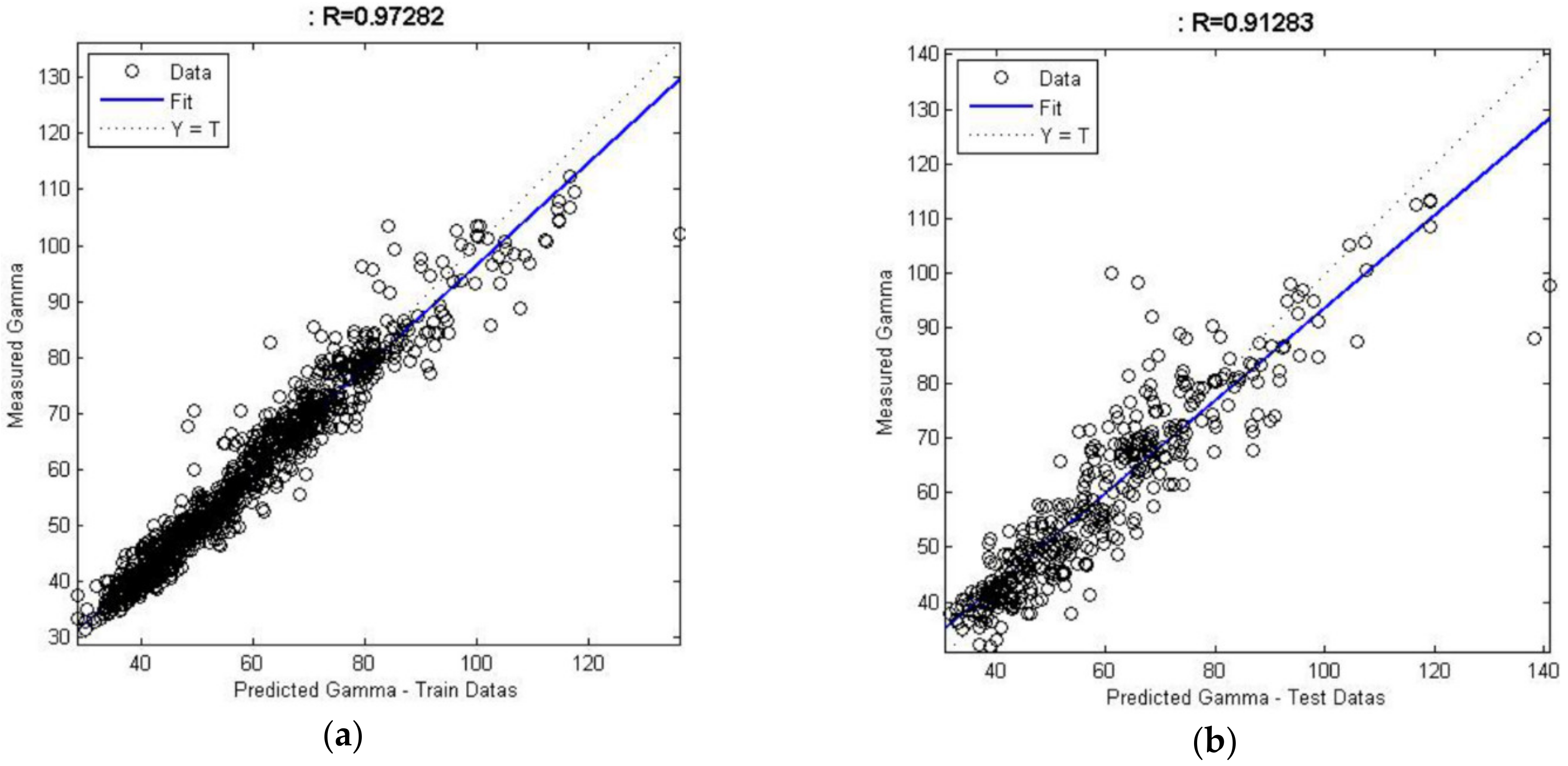
4.2.1. Estimation by General Regression Neural Network (GRNN)

Due to the need to determine the optimal radius to estimate the best application of this method, different values from 0 to 1 were selected. The optimal value of 0.015 was selected for the optimum radius. Figure 16 shows the estimated continuous line and the actual point values in the training and test data.

To present a better view of the accuracy of the estimation, a comparison between the estimated values and the actual values for each coordinate in the two categories of training and test data is given in regression in Figure 17, respectively. The accuracy (R) of these estimates was 0.97 in the training data and 0.91 in the test data.

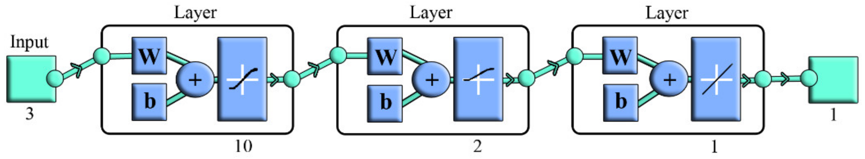
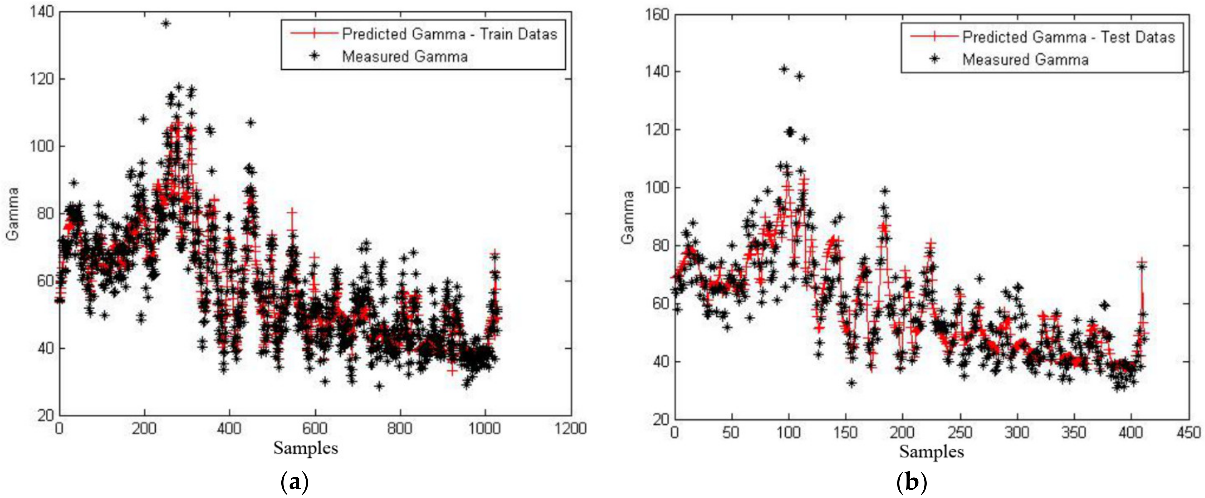
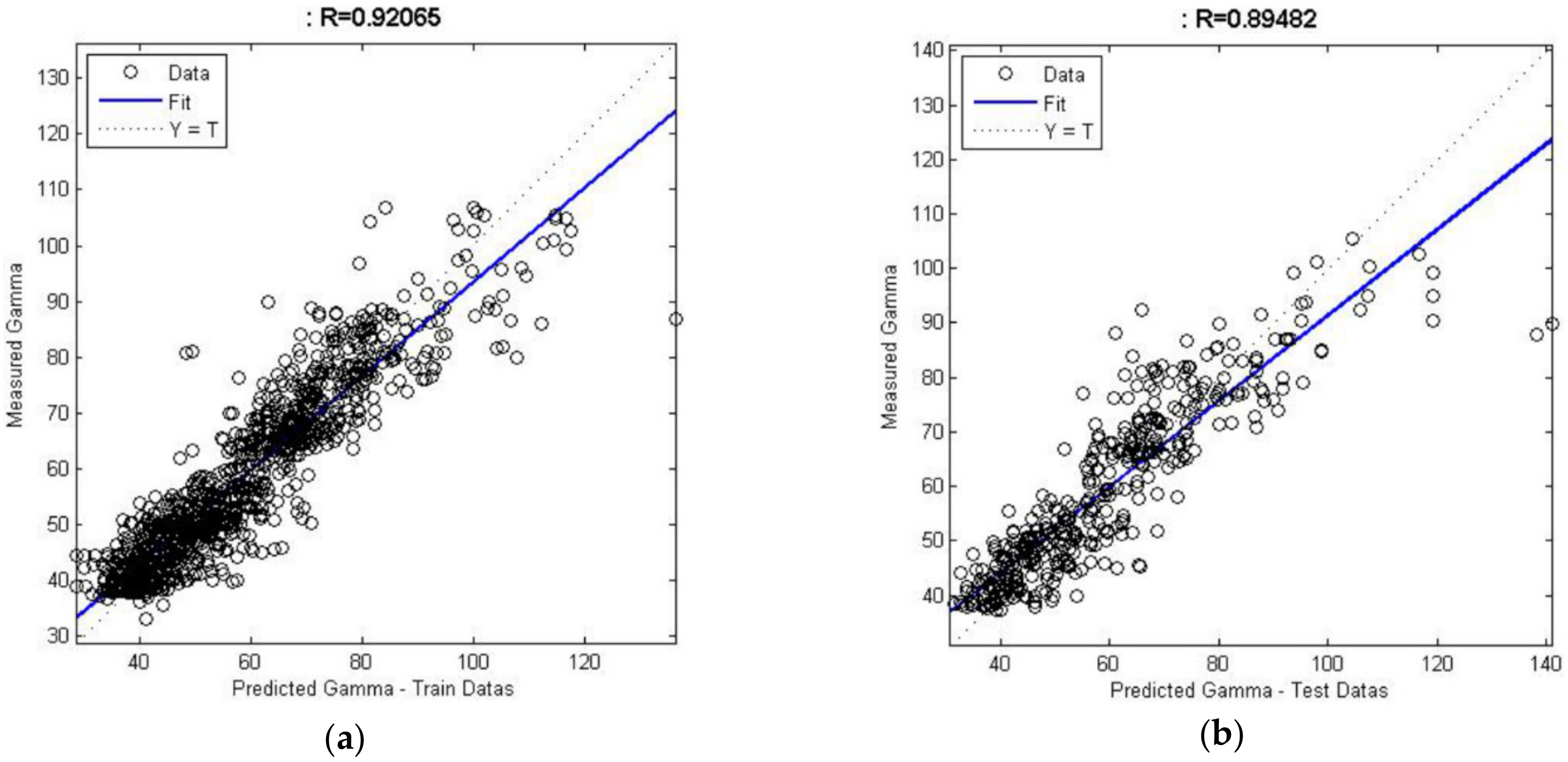
4.2.2. Estimation by Backpropagation Neural Network (BPNN)

In this method, parameters, such as the type of training, the number of neurons in different layers, and the type of neurons, are important. In the following results, the network efficiency is estimated by the average error squares (which is automatically calculated and minimized, and, if the average error squares is inappropriate, the network will remain endless) and the type and number of neurons. A schematic representation of BPNN is shown in Figure 18.

To check for no over-fitting in the existing network, the number of iterations of permissible neural network epochs was considered repeatedly. As a result, the network training ended in 201 repetitions, and the error value was in the standard range. The reason for this is the convergence of the estimation network. Therefore, over-fitting has not been done in the artificial neural network.

The results of the estimation line along with the real points in the training and test data are shown in Figure 19, as well as the accuracy of the training and test data, which are estimated to be 0.92 and 0.89 in Figure 20, respectively.

5. Conclusions

Due to radioactive evidence in the Ardakan region located in Yazd province, it is important to study the behavior of magnetometric and radiometric surveys in the region. For this purpose, the behavior of magnetometric and radiometric data in the area of the Toot iron deposit relative to each other was studied using the K-means method. The interaction of these two parameters was presented as an equation with a correlation coefficient. Then, using the K-means method, the relationship between radiometric and magnetometric data was determined by considering the latitude and longitude of the points to more accurately estimate the occurrence and extent of anomalies in the study area. The behavior of these two parameters in the region is such that to increase the intensity of the magnetic field, the intensity of radiation first increases, and after reaching a field intensity of 47,500 nT, it decreases, and after reaching 49,000 nT in the region, it does not cause any unusual behavior.

As presented in this study, the correlation between radiometric and magnetometric data was almost zero. Still, after behavioral studies, it was found that this dependence was zero on average, while the partial behavior in the data shows the dependence. Finally, the intensity of radiation was determined using the methods of GRNN and BPNN based on the magnetic measurement, length, and width of the points. The accuracy (R) of the estimation in the test data in the GRNN is 0.91, and, in the BPNN, it is 0.89. In addition to showing the strength of the K-means clustering method in behavioral studies, these results are superior to those produced using the general regression neural network (GRNN) method in the optimal estimation of radiation intensity based on magnetometric data in the region.

References

1. Mohammadi, N.M.; Hezarkhani, A.; Maghsoudi, A. Application of K-means and PCA approaches to estimation of gold grade in Khooni district (central Iran). Acta Geochim. 2018, 37, 102–112. [Google Scholar] [CrossRef]
2. Khakmardan, S.; Doodran, R.J.; Shirazy, A.; Shirazi, A.; Mozaffari, E. Evaluation of Chromite Recovery from Shaking Table Tailings by Magnetic Separation Method. Open J. Geol. 2020, 10, 1153–1163. [Google Scholar] [CrossRef]
3. Shirazi, A.; Shirazy, A.; Saki, S.; Hezarkhani, A. Geostatistics Studies and Geochemical Modeling Based on Core Data, Sheytoor Iron Deposit, Iran. J. Geol. Resour. Eng. 2018, 6, 124–133. [Google Scholar]
4. Ziaii, M.; Safari, S.; Timkin, T.; Voroshilov, V.; Yakich, T. Identification of geochemical anomalies of the porphyry–Cu deposits using concentration gradient modelling: A case study, Jebal-Barez area, Iran. J. Geochem. Explor. 2019, 199, 16–30. [Google Scholar] [CrossRef]
5. Malyszko, D.; Wierzchon, S.T. Standard and Genetic K-means Clustering Techniques in Image Segmentation. In Proceedings of the 6th International Conference on Computer Information Systems and Industrial Management Applications, Elk, Poland, 28–30 June 2007; IEEE Computer Society: Washington, DC, USA, 2007; pp. 299–304. [Google Scholar]
6. Khakmardan, S.; Shirazi, A.; Shirazy, A.; Hosseingholi, H. Copper Oxide Ore Leaching Ability and Cementation Behavior, Mesgaran Deposit in IRAN. Open J. Geol. 2018, 8, 841–858. [Google Scholar] [CrossRef] [Green Version]
7. Doodran, R.J.; Khakmardan, S.; Shirazi, A.; Shirazy, A. Minimalization of Ash from Iranian Gilsonite by Froth Flotation. J. Miner. Mater. Charact. Eng. 2021, 9, 1–13. [Google Scholar] [CrossRef]
8. Abolhassani, B.; Salt, J.E. A simplex K-means algorithm for radio-port placement in cellular networks. In Proceedings of the Canadian Conference on Electrical and Computer Engineering, Canada, University of Saskatchewan, Saskatoon, SK, Canada, 1–4 May 2005; pp. 2117–2121. [Google Scholar]
9. Wang, Q.; Deng, J.; Liu, H.; Yang, L.; Wan, L.; Zhang, R. Fractal models for ore reserve estimation. Ore Geol. Rev. 2010, 37, 2–14. [Google Scholar] [CrossRef]
10. Shirazy, A.; Ziaii, M.; Hezarkhani, A.; Timkin, T. Geostatistical and Remote Sensing Studies to Identify High Metallogenic Potential Regions in the Kivi Area of Iran. Minerals 2020, 10, 869. [Google Scholar] [CrossRef]
11. Nasor, M.; Obaid, W. Detection and Localization of Early-Stage Multiple Brain Tumors Using a Hybrid Technique of Patch-Based Processing, k-means Clustering and Object Counting. Int. J. Biomed. Imaging 2020, 2020, 1–9. [Google Scholar] [CrossRef] [Green Version]
12. Khorshidi, N.; Parsa, M.; Lentz, D.R.; Sobhanverdi, J. Identification of heavy metal pollution sources and its associated risk assessment in an industrial town using the K-means clustering technique. Appl. Geochem. 2021, 135, 105113. [Google Scholar] [CrossRef]
13. Shirazi, A.; Hezarkhani, A.; Shirazy, A. Remote Sensing Studies for Mapping of Iron Oxide Regions, South of Kerman, IRAN. Int. J. Sci. Eng. Appl. 2018, 7, 45–51. [Google Scholar] [CrossRef]
14. Shirazi, A.; Shirazy, A.; Karami, J. Remote sensing to identify copper alterations and promising regions, Sarbishe, South Khorasan, Iran. Int. J. Geol. Earth Sci. 2018, 4, 36–52. [Google Scholar]
15. Shirazy, A.; Shirazi, A.; Heidar laki, S.; Ziaii, M. Exploratory Remote Sensing Studies to Determine the Mineralization Zones around the Zarshuran Gold Mine. Int. J. Sci. Eng. Appl. 2018, 7, 274–279. [Google Scholar] [CrossRef]
16. Yang, J.; Zhuang, Y.; Wu, F. ESVC-based extraction and segmentation of texture features. Comput. Geosci. 2012, 49, 238–247. [Google Scholar] [CrossRef]
17. Dumuid, D.; Olds, T.; Lewis, L.K.; Martin-Fernández, J.A.; Barreira, T.; Broyles, S.; Chaput, J.-P.; Fogelholm, M.; Hu, G.; Kuriyan, R.; et al. The adiposity of children is associated with their lifestyle behaviours: A cluster analysis of school-aged children from 12 nations. Pediatr. Obes. 2018, 13, 111–119. [Google Scholar] [CrossRef] [PubMed]
18. Ghezelbash, R.; Maghsoudi, A.; Carranza, E.J.M. Mapping of single- and multi-element geochemical indicators based on catchment basin analysis: Application of fractal method and unsupervised clustering models. J. Geochem. Explor. 2019, 199, 90–104. [Google Scholar] [CrossRef]
19. Shirazi, A.; Hezarkhani, A.; Shirazy, A. Exploration Geochemistry Data-Application for Cu Anomaly Separation Based On Classical and Modern Statistical Methods in South Khorasan, Iran. Int. J. Sci. Eng. Appl. 2018, 7, 39–44. [Google Scholar] [CrossRef]
20. Sfidari, E.; Kadkhodaie-Ilkhchi, A.; Najjari, S. Comparison of intelligent and statistical clustering approaches to predicting total organic carbon using intelligent systems. J. Pet. Sci. Eng. 2012, 86, 190–205. [Google Scholar] [CrossRef]
21. Wegner, T.; Hussein, T.; Hämeri, K.; Vesala, T.; Kulmala, M.; Weber, S. Properties of aerosol signature size distributions in the urban environment as derived by cluster analysis. Atmos. Environ. 2012, 61, 350–360. [Google Scholar] [CrossRef]
22. Isaeva, E.R.; Voroshilov, V.G.; Timkin, T.V.; Ziaii, M. Geochemical criteria to identify reservoirs and to forecast their oil and gas content in terrigenous deposits in Pur-Tazovskoy oil-bearing field. Bull. Tomsk. Polytech. Univ. Geo Assets Eng. 2018, 329, 132–141. [Google Scholar]
23. Ghannadpour, S.S.; Hezarkhani, A.; Farahbakhsh, E. An investigation of Pb geochemical behavior respect to those of Fe and Zn based on k-Means clustering method. J. Tethys 2013, 1, 291–302. [Google Scholar]
24. Mora, J.L.; Armas-Herrera, C.M.; Guerra, J.A.; Rodríguez-Rodríguez, A.; Arbelo, C.D. Factors affecting vegetation and soil recovery in the Mediterranean woodland of the Canary Islands (Spain). J. Arid Environ. 2012, 87, 58–66. [Google Scholar] [CrossRef]
25. Al-Alawi, S.M.; Tawo, E.E. Application of Artificial Neural Networks in Mineral Resource Evaluation. J. King Saud Univ. Eng. Sci. 1998, 10, 127–138. [Google Scholar] [CrossRef]
26. Shirazi, A.; Shirazy, A.; Saki, S.; Hezarkhani, A. Introducing a software for innovative neuro-fuzzy clustering method named NFCMR. Glob. J. Comput. Sci. Theory Res. 2018, 8, 62–69. [Google Scholar] [CrossRef]
27. Shirazy, A.; Ziaii, M.; Hezarkhani, A. Geochemical Behavior Investigation Based on K-means and Artificial Neural Network Prediction for Copper, in Kivi region, Ardabil province, IRAN. Iran. J. Min. Eng. 2020, 14, 96–112. [Google Scholar]
28. Hao, X.; Yang, Y.; Li, Y.; Wang, Q. Magnetic anomaly characteristics and iron ore prediction of Chengwu-Caoxian county area in Shandong province, China. Prog. Geophys. 2018, 33, 613–619. [Google Scholar]
29. Kozhevnikov, N.O.; Kharinsky, A.V.; Snopkov, S.V. Geophysical prospection and archaeological excavation of ancient iron smelting sites in the Barun-Khal valley on the western shore of Lake Baikal (Olkhon region, Siberia). Archaeol. Prospect. 2019, 26, 103–119. [Google Scholar] [CrossRef]
30. Saavedra, S.; Rincón, P. Interpretation of geophysical anomalies for mineral resource potential evaluation in Colombia: Examples from the northern Andes and Amazonian regions. Boletín Geológico 2020, 46, 5–22. [Google Scholar]
31. Martin, P.G.; Connor, D.T.; Estrada, N.; El-Turke, A.; Megson-Smith, D.; Jones, C.P.; Kreamer, D.K.; Scott, T.B. Radiological identification of near-surface mineralogical deposits using low-altitude unmanned aerial vehicle. Remote. Sens. 2020, 12, 3562. [Google Scholar] [CrossRef]
32. Jekeli, C.; Erkan, K.; Huang, O. Gravity vs pseudo-gravity: A comparison based on magnetic and gravity gradient measurements. Gravity Geoid Earth Obs. 2010, 135, 123–127. [Google Scholar]
33. Dowling, R.K. Geotourism’s Global Growth. Geoheritage 2011, 3, 1–13. [Google Scholar] [CrossRef]
34. Shirazi, A.; Shirazy, A. Introducing Geotourism Attractions in Toroud Village, Semnan Province, IRAN. Int. J. Sci. Eng. Appl. 2020, 9, 79–86. [Google Scholar] [CrossRef]
35. Nabatian, G.; Rastad, E.; Neubauer, F.; Honarmand, M.; Ghaderi, M. Iron and Fe–Mn mineralisation in Iran: Implications for Tethyan metallogeny. Aust. J. Earth Sci. 2015, 62, 211–241. [Google Scholar] [CrossRef]
36. Ghorbani, M. The Economic Geology of Iran; Springer Geology; Springer: Dordrecht, The Netherlands, 2013. [Google Scholar]
37. Ghorbani, M. A Summary of Geology of Iran; Springer: Dordrecht, The Netherlands, 2013; pp. 45–64. [Google Scholar]
38. Nabavieh, S.M.; Mehdi Abad, H.T. Geological Map (on Scale 1:100000) 2003; Geological Survey and Mineral Exploration of Iran (GSI): Tehran, Iran, 2003. [Google Scholar]
39. Myers, L.; Sirois, M.J. Spearman Correlation Coefficients, Differences between. In Encyclopedia of Statistical Sciences; John Wiley & Sons, Inc.: Hoboken, NJ, USA, 2006. [Google Scholar]
40. Alahgholi, S.; Shirazy, A.; Shirazi, A. Geostatistical Studies and Anomalous Elements Detection, Bardaskan Area, Iran. Open J. Geol. 2018, 8, 697–710. [Google Scholar] [CrossRef] [Green Version]
41. Shirazy, A.; Shirazi, A.; Hezarkhani, A. Predicting gold grade in Tarq 1: 100000 geochemical map using the behavior of gold, Arsenic and Antimony by K-means method. J. Miner. Resour. Eng. 2018, 2, 11–23. [Google Scholar]
42. Zhou, S.; Zhou, K.; Wang, J.; Yang, G.; Wang, S. Application of cluster analysis to geochemical compositional data for identifying ore-related geochemical anomalies. Front. Earth Sci. 2018, 12, 491–505. [Google Scholar] [CrossRef]
43. Jain, A.K. Data clustering: 50 years beyond K-means. Pattern Recognit. Lett. 2010, 31, 651–666. [Google Scholar] [CrossRef]
44. Shirazy, A.; Ziaii, M.; Hezarkhani, A.; Timkin, T.V.; Voroshilov, V.G. Geochemical behavior investigation based on K-means and artificial neural network prediction for titanium and zinc, Kivi region, Iran. Bull. Tomsk Polytech. Univ. Geo Assets Eng. 2021, 332, 113–125. [Google Scholar]
45. Saha, S.; Bandyopadhyay, S. A generalized automatic clustering algorithm in a multiobjective framework. Appl. Soft Comput. 2013, 13, 89–108. [Google Scholar] [CrossRef]
46. Hezarkhani, A.; Ghannadpour, S.S. Geochemical Behavior Investigation Based on K-Means Clustering: Basics, Concepts and Case Study; LAP LAMBERT Academic Publishing: Frankfurt, Germany, 2015; 60p. [Google Scholar]
47. Shirazy, A.; Shirazi, A.; Hezarkhani, A. Behavioral Analysis of Geochemical Elements in Mineral Exploration; LAP LAMBERT Academic Publishing: Saarbrücken, Germany, 2020. [Google Scholar]
48. Beale, M.Y.; Hagan, M.T.; Demuth, H.B. Neural Network Toolbox User’s Guide; The MathWorks: Natick, MA, USA, 2010; 846p. [Google Scholar]
49. Specht, D.F. A General Regression Neural Network. IEEE Trans. Neural Netw. 1991, 2, 568–576. [Google Scholar] [CrossRef] [Green Version]
50. Rooki, R. Application of general regression neural network (GRNN) for indirect measuring pressure loss of Herschel–Bulkley drilling fluids in oil drilling. Measurement 2016, 85, 184–191. [Google Scholar] [CrossRef]
51. Mohammadi, N.M.; Hezarkhani, A. Estimation of grade Gold in khooni deposit using the behavior of gold, Arsenic and Antimony elements by clustering K-means method. J. Anal. Numer. Methods Min. Eng. 2015, 5, 77–92. [Google Scholar]
Figure 1. Overview geological map of the iron deposits of Iran and the Toot area (modified after Reference [35]).
Minerals 11 01304 g001
Figure 2. Geological map of the study area Toot.
Minerals 11 01304 g002
Figure 3. Field photographs of rocks containing iron mineralization. (a) Detailed view of the metamorphic unit of the shale and between its thin dolomite layers as the host of the iron anomaly. (b) A closer look at magnetite mineralization in a metamorphic shale unit.
Minerals 11 01304 g003
Figure 4. Primary and oxidized iron ore. Banded and frequency mineralization of magnetite and quartz (a); (b) weathering in magnetite and replaced by hematite and limonite.
Minerals 11 01304 g004
Figure 5. Distribution of economic minerals in the thin section and polish section of different samples. Mt = magnetite; Act = actinolite; Chl = chlorite; Bt = biotite. (a) Actinolite crystals co-growth between coarse chlorite crystals; (b) occurrence of pyrite mineralization in the form of a strip or lens; (c) magnetite crystals in the space between biotite crystals; (d) chlorite crystals between opaque ores (magnetite); (e) accumulation magnetite crystals in subhedral; (f) magnetite interlayers.
Minerals 11 01304 g005
Figure 6. Location of the study area near the Toot village (image: Landsat/ Copernicus).
Minerals 11 01304 g006
Figure 7. Histogram of magnetometric and radiometric data.
Minerals 11 01304 g007
Figure 8. Schematic of K-Means clustering algorithm.
Minerals 11 01304 g008
Figure 9. Radial neural network structure (schematic).
Minerals 11 01304 g009
Figure 10. Types of activation functions for example (modified after References [46,47]).
Minerals 11 01304 g010
Figure 11. Cluster profiles and utility values with 3 to 6 classes related to magnetometric and radiometric recording without coordinates. (a) Classification with 3 classes with an average value of 0.6965; (b) classification with 4 classes with an average value of 0.8830; (c) classification with 5 classes with an average value of 0.7732; (d) classification with 6 classes with an average value of 0.7672 (values are dimensionless between −1 to 1).
Minerals 11 01304 g011aMinerals 11 01304 g011b
Figure 12. Cluster profiles and utility values with 3 to 6 classes related to magnetometric and radiometric recording with coordinates. (a) Classification with 5 classes with an average value of 0.4141; (b) classification with 6 classes with an average value of 0.6220 (values are dimensionless between −1 to 1).
Minerals 11 01304 g012
Figure 13. The value of S (i) (vertical axis) is based on the number of clusters (horizontal axis), the intensity of radioactivity, and the intensity of the magnetic field ((a): no coordinates, (b): with coordinates). (S (i) is dimensionless).
Minerals 11 01304 g013
Figure 14. Four separated classes on the geological map.
Minerals 11 01304 g014
Figure 15. The best-fitting line to the centers of the categories for measurements.
Minerals 11 01304 g015
Figure 16. Gamma (Bq/Kg) estimation line with real values in training (a) and test (b) data.
Minerals 11 01304 g016
Figure 17. Regression of estimated Gamma versus real Gamma (Bq/Kg); (a) Training, (b) Test.
Minerals 11 01304 g017
Figure 18. Schematic figure of Backpropagation Neural Network (BPNN) used in this study. (A network with an input layer and two hidden layers, the first layer has 10 neurons and the second layer has 2 neurons. The output layer is linear. In addition, in each neuron is shown schematically, weight and bias.)
Minerals 11 01304 g018
Figure 19. Radiation intensity estimation line with real values of the training (a) and (b)test data. (Bq/Kg.)
Minerals 11 01304 g019
Figure 20. Regression of estimated data versus real; (a) Training, (b) Test. (Bq/Kg.)
Minerals 11 01304 g020