Model Scaling in Smartphone GNSS-Aided Photogrammetry for Fragmentation Size Distribution Estimation

Abstract

Fragmentation size distribution estimation is a critical process in mining operations that employ blasting. In this study, we aim to create a low-cost, efficient system for producing a scaled 3D model without the use of ground truth data, such as GCPs (Ground Control Points), for the purpose of improving fragmentation size distribution measurement using GNSS (Global Navigation Satellite System)-aided photogrammetry. However, the inherent error of GNSS data inhibits a straight-forward application in Structure-from-Motion (SfM). To overcome this, the study proposes that, by increasing the number of photos used in the SfM process, the scale error brought about by the GNSS error will proportionally decrease. Experiments indicated that constraining camera positions to locations, relative or otherwise, improved the accuracy of the generated 3D model. In further experiments, the results showed that the scale error decreased when more images from the same dataset were used. The proposed method is practical and easy to transport as it only requires a smartphone and, optionally, a separate camera. In conclusion, with some modifications to the workflow, technique, and equipment, a muckpile can be accurately recreated in scale in the digital world with the use of positional data.

1. Introduction

Fragmentation size is a key parameter to the efficiency of numerous mining operations that makes use of explosives across all of the stages of production from mine (drill, blasting, haulage, etc.) to mill (mineral processing). Several studies [1,2] going back to the late 1990s have explored this particular correlation. It is vital for companies, therefore, to monitor fragmentation size and make necessary changes to mine planning and execution. For the purpose of maintaining a consistent optimal fragmentation size, the blasting products must be monitored regularly, so that any necessary modifications to the drilling and blasting process can be made.

However, the rock is usually heterogeneous in nature, and a large amount of material is generally mined every day, so there are some difficulties in monitoring the fragmentation size distribution regularly using traditional methods. These traditional methods include manual sieving, boulder counting, and visual estimation. However, limitations on sampling and bias make these methods relatively inefficient [3]. As such, there exists a need for a quick and accessible method of rock fragmentation size distribution determination that can surmount the limitations of physical sampling and laboratory analysis. A currently used digital solution to this problem is to employ image-based particle size analysis software.

Commercial products, such as WipFrag [4], make use of images of a muckpile or orthomosaics to measure fragmentation size distribution. In addition, other 3D modelling technologies, such as lidar systems, have also been used in fragmentation measurement systems producing good results and accurate measurements without the need for scale objects.

A previous study [5] was done using laser scanning to measure the blast fragmentation in rockpiles in a mine. While specialized equipment was used to do this study, lidar is becoming increasingly accessible in recent years, with newer generation smartphone models including a lidar system. The study recognizes that this is also a good alternative to perform fragmentation measurement as they are potentially effective in an underground setting where lighting is limited, an issue that produces problems for traditional image-based photogrammetry [6].

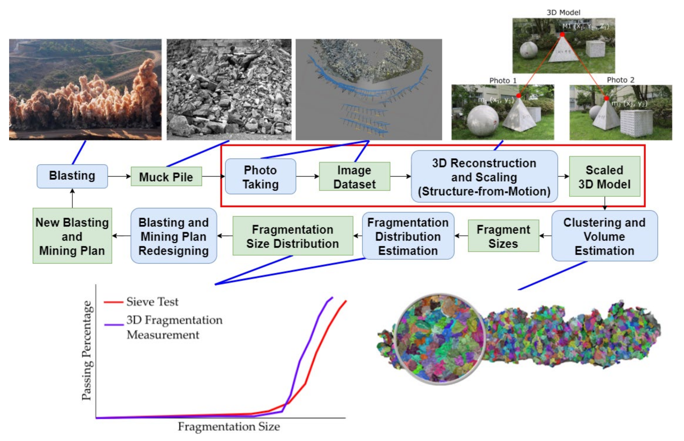
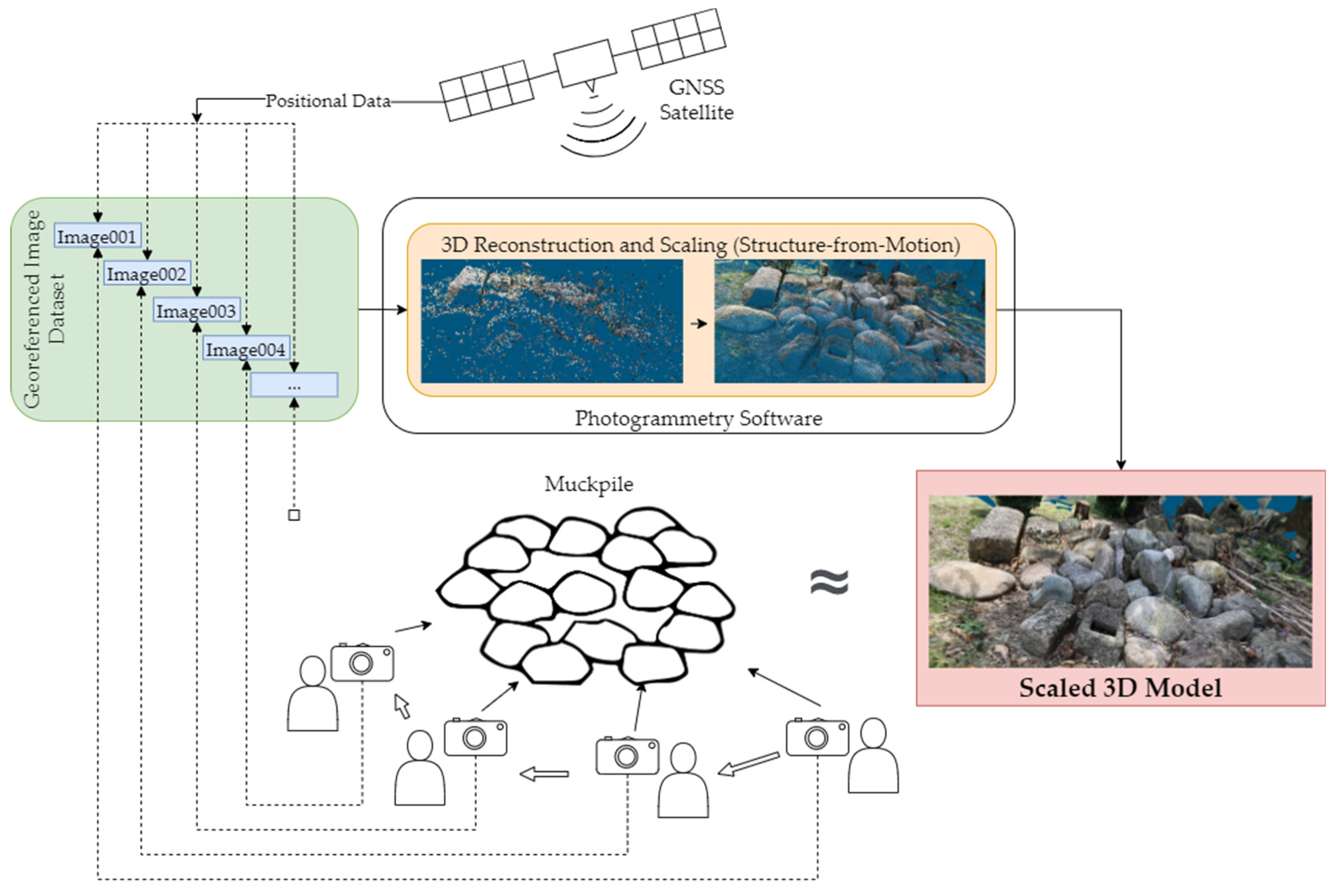
In a previous study [7], a 3-Dimensional Fragmentation Measurement (3DFM) system was developed that makes use of 3D Photogrammetry to measure particle size distribution at accuracies greater than that of conventional methods. A theoretical visualized workflow for this particular system when applied to a mining operation is shown in Figure 1.

The developed system is divided into stages, utilizing multiple computational techniques in order to achieve its purpose. In a hypothetical application of the system, pictures of the muckpile from the products of blasting are taken. The sizes of muckpiles vary greatly depend on the specifications of the hauling equipment as well as the mine plan that the operation employs. In situations where the muckpile is too large or has parts that are inaccessible to photo-taking, it is possible for the system to reconstruct only a representative “slice” of the muckpile.

The images are then processed in a high-power computer by a sequence of 3D imaging techniques that will ultimately output a scaled 3D model of the muckpile in the form of a point cloud. A technique known as supervoxel clustering is then performed on the 3D model, which then undergoes supervoxel clustering in order to divide the individual fragments into segments whose dimensions have been calculated. The dimensional data can then be used in the computation of the fragment size distribution of the muckpile. Using this information, the blasting product can be judged if it is up to the expected specification. Adjustments are then made the blasting design, such as the amount and type of explosive and blasting patterns in order to achieve the required distribution.

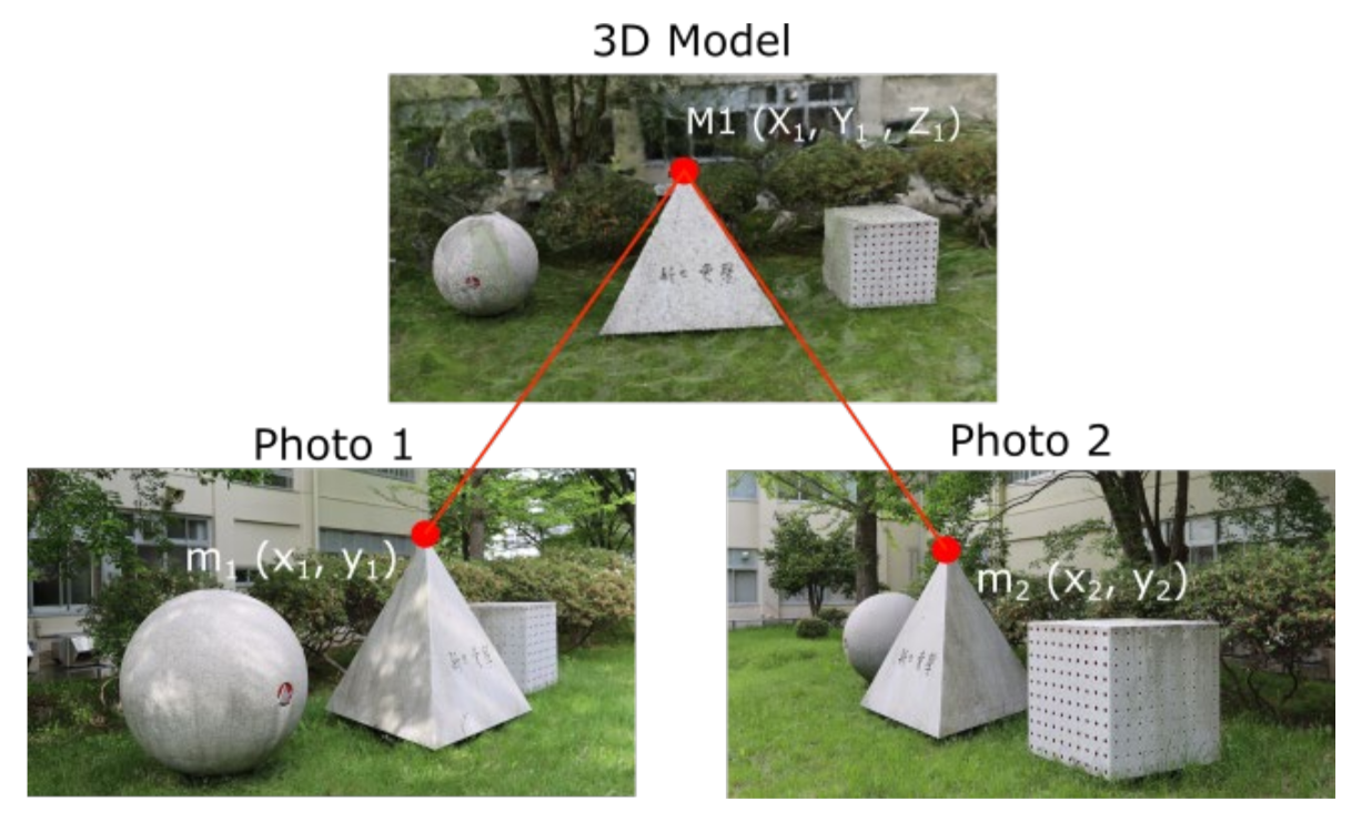
This study focuses on the 3D model scaling aspect of this system, as highlighted with a red box in Figure 1. Specifically, the research will analyze how positional data can affect scaling error when reconstructing using Structure-from-Motion. Scaling is a critical component of fragmentation size distribution measurement using photogrammetry as this will directly determine the accuracy of the size estimation. In creating a 3D model, extrinsic data, such as ground truths, are needed to create a properly-scaled reconstruction of the scene. Traditionally, scale is resolved in photogrammetry by placing scale bars in the scene or taking a measurement of two features and then scaling the generated model using that information.

The study proposes a method that makes use of GNSS (Global Navigation Satellite System) data to create scaled 3D models without the need for post-reconstruction rescaling. GNSS positional data, and its sub-systems, such as GPS, Beidou, GLONASS, and Japan’s own QZSS can be utilized. A previous study was performed with regards to using GPS in reconstruction but mostly in the context of UAV (Unmanned Aerial Vehicle) Mapping [8]. This study aims to create a system that does not need ground truth data, such as GCPs (Ground Control Points) to create a properly scaled 3D model of a muckpile. This would aid greatly in the fragmentation size distribution measurement of muckpiles using photogrammetry.

It is a known fact that inherent error exists within GNSS and its subsets, and even high-end geodetic GNSS receivers have errors in the centimeter range [9]. For this study, a smartphone was used as a GNSS receiver for the digital camera. This decision was due to the end-goal of this research, which is to be able use both image data and GNSS data from a smartphone, as this practicality can be important in a mining operation environment.

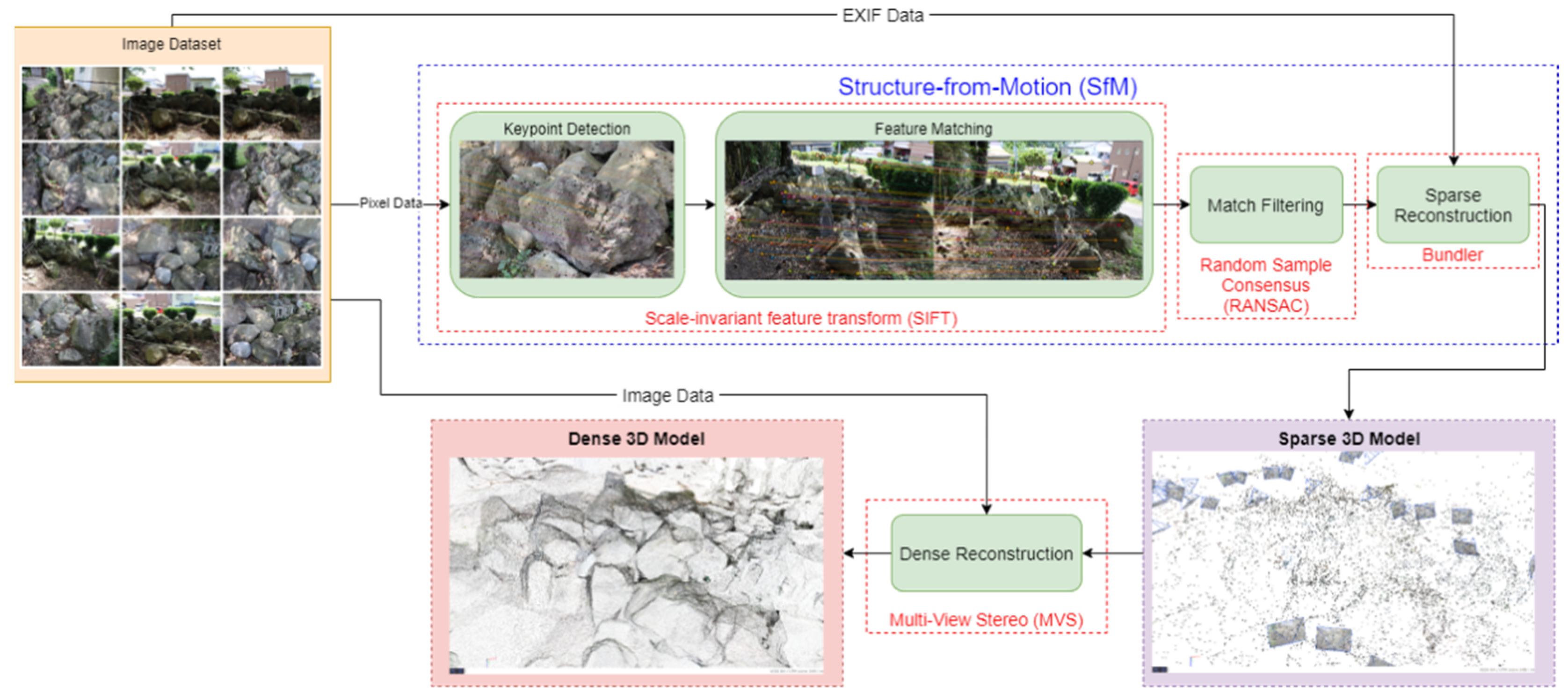
This comes at a drawback to the GNSS accuracy, as recreational grade GNSS chips, like those found in smartphones, typically have errors in the meter range [10]. To overcome this error, the study proposes to make use of an increasing number of georeferenced images to statistically decrease the scaling error of the constructed 3D model. Figure 2 shows a general overview of the proposed system for this study. Utilizing a smartphone’s built-in GNSS receiver, GNSS data can be logged and sent to a camera. At the moment an image is taken, GNSS data can be embedded into the image’s metadata (EXIF).

In a similar study [11], a Real Time Kinematic (RTK) GNSS receiver was used in conjunction with a camera for a photogrammetric survey of a geological outcrop. The method suggested in this study is a potentially cheaper alternative as it utilizes the built-in GNSS receiver in a smartphone. In a similar fashion, the method used by this study allows for greater flexibility as it is a point-and-shoot method that does not require external preparation. While this can mean that more photos will be needed to generate a 3D model, the cost-efficiency and the practicality of not having to use GCPs or physical scales can be desirable in some applications.

2. Materials and Methods

2.1. Structure-from-Motion—Multi View Stereo (SfM-MVS)

Mathematically speaking, SfM can be described as the conversion of four coordinate systems, illustrated in Figure 3:

(1)

An image pixel coordinate system, which concerns the pixels on the 2D image.

(2)

An imaging plane coordinate system, which lie on the same plane of the previous system, but whose origin is the plane’s intersection with the camera’s optical axis.

(3)

A camera coordinate system, which concerns a pinhole camera’s point of view of the image.

(4)

A world coordinate system, which is a reference system to describe the position of the camera and the objects being taken pictures of.

$$Z_c\left[\begin{array}{c}u\\ v\\ 1\end{array}\right]=\left[\begin{array}{ccc}\frac{1}{{\delta }_x}& 0& u_o\\ 0& \frac{1}{{\delta }_y}& v_o\\ 0& 0& 1\end{array}\right]\left[\begin{array}{ccc}f& 0& 0\\ 0& f& 0\\ 0& 0& 1\end{array}\right]\left[\begin{array}{cc}\mathit{R}& \mathit{t}\end{array}\right]\left[\begin{array}{c}{X}_w\\ Y_w\\ Z_w\\ 1\end{array}\right]=\left[\begin{array}{ccc}{f}_x& 0& u_0\\ 0& f_y& v_0\\ 0& 0& 1\end{array}\right]\left[\begin{array}{cc}\mathit{R}& \mathit{t}\end{array}\right]\left[\begin{array}{c}{X}_w\\ Y_w\\ Z_w\\ 1\end{array}\right]$$

(1)

The conversion of these four coordinates systems can be described by Equation (1). $u$ and $v$ describe the axes in the imaging planes. $u_0$ and $v_0$ are the coordinates of the origins of the imaging plane in the pixel coordinate system. ${\delta }_x$ and ${\delta }_y$ represent the physical size of each pixel in the image in the imaging plane (zoom ratio). $f$ describes the focal length, which is the distance from the optical center of the camera to the pixel plane. $\mathit{R}\in {ℝ}^{3\times 3}$ and $\mathit{t}\in {ℝ}^3$ describe the rotational and translational vectors that relate the camera and the world coordinate systems. $X_w$, $Y_w$, $Z_w$ are the actual coordinates of a point in the world coordinate system [12].

Equation (1) represents the fact that, in order to estimate the position of a point in the real world, the external parameter matrix of the camera (i.e., R and t) needs to be measured first. Once R is known, the relative position of the object in the world coordinate system can be estimated, and once t is known, the absolute position can also be acquired as well. Basic SfM can relatively estimate R and t. In this study, GNSS data is used as the absolute value of t. The details of this method are described in Section 2.2.

It can be inferred that there is no single ‘correct’ workflow or process in the conversion of 2D images into models. However, there are key processes that are present in almost all applications of the method, as shown in Figure 4. The steps are briefly described in the following sections.

2.1.1. Keypoint Detection

The initial processing step after acquiring the images is feature detection, or extraction, where possible common features (keypoints) in the individual images are identified as shown in Figure 5. It is by these features that allow the different images in the dataset to be matched at the next stage. There are several techniques that have been developed for the solution of this step [13]; however, the most widely used amongst modern SfM applications is the scale-invariant feature transform (SIFT) [14].

The system recognizes feature points in the image set, which are uniform in scaling and rotation and relatively uniform to changes in lighting and 3D camera view angles. The number of keypoints that are extracted in an image relies heavily on the resolution and texture of the images themselves with high-quality, original-resolution pictures returning the most results [15].

2.1.2. Keypoint Matching

The next step is to match the keypoints and identify the correspondences between them. Matches are found by identifying a keypoint’s nearest neighbor in the database. The nearest neighbor is defined as the keypoint with the least Euclidean distance for its descriptor vector, as shown in Figure 6 [14]. It is also important to note at this point that not all keypoints are guaranteed to have a good match in the dataset. It is, therefore, necessary to discard these unmatched keypoints, making use of the ratio between the Euclidean distance of the nearest neighbor with that of the second nearest at a certain minimum value as a criterion for discarding false keypoint matches [13].

The inherent complexity of the keypoint descriptors gives rise to the need of an efficient solution to the search process, as brute-force searching for nearest neighbors proves to be computationally difficult and time-consuming. Several solutions, such as k-dimensional trees (k-d trees), best-bin first (BBF), and approximate nearest neighbor (ANN) searching, are used to solve this problem of efficiency by partitioning the data into bins that are prioritized for match searching, thus, decreasing the number of recursions needed to go through all the keypoints [13].

2.1.3. Keypoint Filtering

The third stage, also known as geometric verification or match filtering, is done to further eliminate erroneous matches. Since the initial matching is solely based on appearance, it cannot be guaranteed that the matched keypoints refer to the same point in an image (e.g., images with symmetrical or similar features) [16]. SfM then needs to verify matches by mapping keypoints across images using projective imagery. An example of this step can be illustrated by the image pair in Figure 7. The two images are of the same scene, taken at two different angles, and the keypoints found in both images are matched, as shown by colored matching tracks.

2.1.4. Sparse Reconstruction: Structure-from-Motion

The fourth step, which also by itself is sometimes called SfM (Structure-from-Motion), is to reconstruct the scene that was taken using 2D images into an initial sparse 3D structure. Using the verified matched keypoints, SfM aims to simultaneously reconstruct the: (a) 3D scene structure, (b) camera position and orientation (extrinsic parameters), and (c) intrinsic camera calibration parameters. The intrinsic camera parameters are defined by a camera calibration matrix that includes image scale, skew, and the principal point that is defined as the location on the image plane that intersects the optical axis.

Further intrinsic parameters are also required to resolve additional internal aberrations, such as distortion on non-pre-calibrated cameras. These intrinsic parameters are either included in the camera’s image file format (e.g., EXIF) or will be resolved in additional intermediate steps. After this, a process known as bundle adjustment is used to produce sparse point-clouds [16]. This process will be described further in another part of the paper below as it is in this step that GNSS constraints will come to play in scaling the produced 3D model. A simplified illustration of this process is described by the illustration in Figure 8.

2.1.5. Dense Reconstruction: Multi View Stereo

An additional, post-processing method known as MVS (Multi-View Stereo) can be applied to the sparse 3D model from SfM in order to generate an enhanced “dense” 3D model. The final output of MVS is a complete 3D scene reconstruction from a collection of images of known intrinsic and extrinsic parameters, which is already resolved through SfM. A variety of MVS algorithms are available but recent variants called clustering views for MVS (CMVS), and patch-based MVS (PMVS) was observed to perform well against other algorithms [13].

CMVS decomposes the camera poses from bundle adjustment into manageable clusters, and PMVS is used to independently reconstruct the 3-dimensional model from these clusters [15]. Most modern MVS pipelines, including the one in the software used for this study, include features from both these variants of MVS. A comparison of the point density between sparse and dense reconstructions is illustrated in Figure 9.

2.2. GNSS-Aided Scaling in Bundle Adjustment

In the bundle adjustment phase of SfM, the previous and imperfect solutions regarding camera positions and 3D features of the scene are refined [17]. More specifically, bundle adjustment is a non-linear minimization procedure that jointly optimizes the camera parameters and point position by minimizing the reprojection error between the image locations of observed and predicted image points. This minimization is done using nonlinear least-squares algorithms [18].

Numerous studies have been done since its inception in the 1990s regarding bundle adjustment, with most of the research going into reducing its computational burden and accelerating the problem-solving process [19]. One of such propositions is the fusion of positional data and bundle adjustment, with GNSS data being used as constraints for solving reprojection errors [20]. This concept is what this research aims to produce: accurately-scaled 3D reconstructions of muckpiles. GNSS data is used to provide position and covariance estimates for the bundle adjustment process. The nominal form of these solutions is:

$$\begin{array}{c}{r}_{GNSS}^M\left(\tau \right)=r_c^M\left(\tau \right)+R_c^M\left(\tau \right)r_{GNSS}^c+\left(b_{GNSS}^M+d_{GNSS}^M\left(\tau -{\tau }_0\right)\right)\end{array}$$

(2)

where $r_{GNSS}^M\left(t\right)$ is the position of the GNSS receiver, $r_c^M\left(t\right)$ denotes the camera position, $R_c^M\left(t\right)$ is the rotational matrix that aligns the camera and mapping space axes, and $r_{GNSS}^c$ is the difference between the GNSS receiver and camera position. $b_{GNSS}^M$ and $d_{GNSS}^M$ denote bias and drift terms and are included to account for data inconsistencies and the inherent errors that exist within GNSS. A previous study [11] applied GNSS-assisted terrestrial photogrammetry to model coastal areas without the use of GCPs. With bundle adjustment being an error minimization problem with multiple factors, weights can be assigned to them, as is the case in the study’s SfM workflow.

The software that was used for this study was developed with the aim of being able to perform SfM without the need for any additional intrinsic or extrinsic data (such as GNSS) aside from the image themselves. [21]. However, the software itself still allows for the importation of GNSS data from images for the purpose of constraining camera positions. Weights are assigned to this GNSS data and used in the bundle adjustment step [22]. As such, the study deems it necessary to initially prove if properly constraining camera positions will help in creating a properly scaled 3D model. A preliminary experiment was designed to test this theory, which is described in the proceeding section of this paper.

Preliminary Experiment for Validating Scaling Fundamentals

A preliminary photogrammetry experiment was performed before the main experiment to test some core concepts regarding the study, specifically the effects of known and constrained camera positions on scaling error and reconstruction quality. This small-scale experiment involved taking photos of a scene that was set-up indoors in the laboratory that consisted of a stuffed dog plush toy that was placed on the floor in such a way that it was in the middle of a grid of nine carpet panels. The panels are 50 by 50 cm in size and form a 3 × 3 grid measuring 150 by 150 cm in total. Figure 10 shows the general layout of the scene. The purpose of this grid is to provide a spatial reference for the camera positions when taking pictures of the scene. A detailed board was put on the middle of the scene to provide enough feature points for SfM, as initial reconstructions without the board resulted in distorted point clouds with missing parts.

The camera used for this preliminary and succeeding experiments was a Canon EOS R equipped with a Canon 24–105 mm lens. The f-stop was set at 4 with variable exposure times, automatic white balancing enabled, and the zoom was kept at a minimum to provide a fixed focal length, which is required for SfM. A total of 32 photos were taken, two at each of the intersection points of the grid at different heights (45 and 60 cm), with sample images shown in Figure 11. The height was maintained by mounting the camera on an adjustable tripod.

Along with the 50 cm spacing, this provided known relative camera positions. The captured images were then processed with a workflow that consisted of making the sparse point cloud and a dense point cloud using photogrammetry software. Creating a textured mesh was deemed unnecessary as it meant a longer processing time and larger project file size and ultimately did not contribute to analyzing the results of the experiment. After this, the camera positions were constrained to their known locations. The scaling error of the reconstructed model was then analyzed.

Without any camera constraints, the software arbitrarily designated a scale, rotation, and translation for the model, and the measurement of the dimension of the carpet panel was about 10 units (since there are no constraints applied, this value cannot be assigned a specific unit of measurement). However, upon adding constraints to the camera (at the centimeter level) by importing a file describing each image’s distance from each other, the same dimension then measured at 51.2719 cm, with a difference of 1.2719 cm from the real measurement of 50 cm.

This difference was attributed to human error during the shooting process. A possible specific example is that the center of the tripod (and, by extension, the center of the camera) was used to align the camera to the grid instead of the nodal point of the camera lens. This means that the images were offset from the actual intended grid position depending on the orientation of the camera and the tripod. Despite this difference, the study still proves fundamentally that accurately constraining the camera positions to their real-world values improved the scale accuracy of the constructed 3D model.

3. GNSS-Constrained SfM on Monuments of Known Dimensions

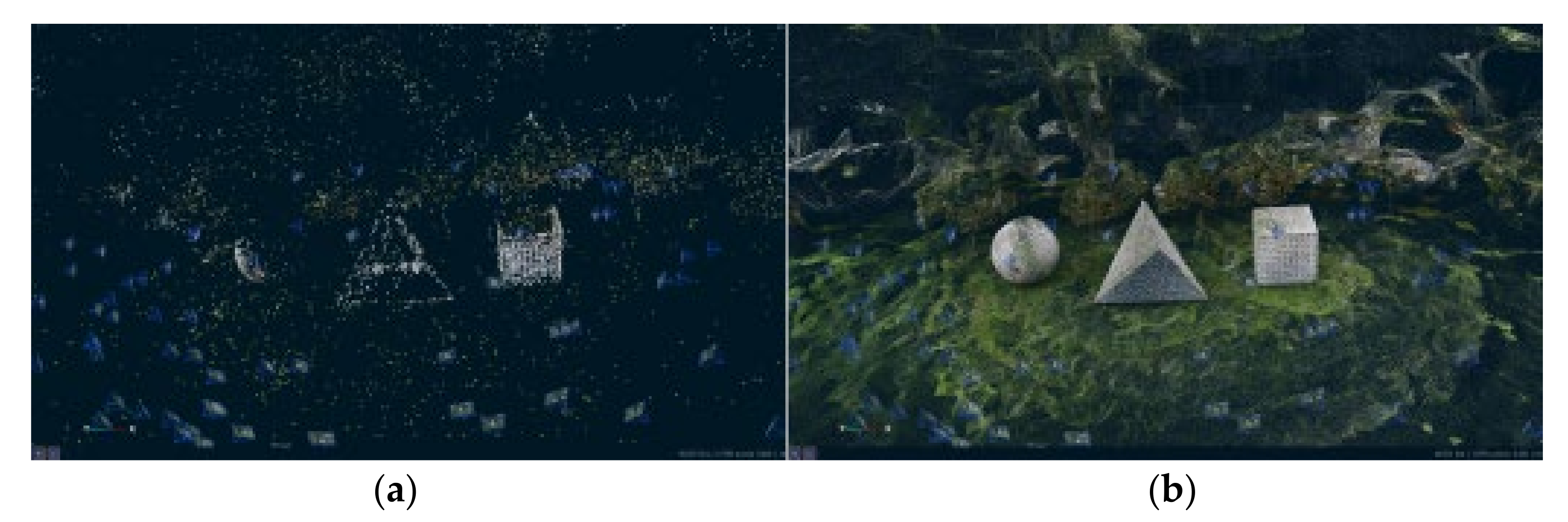
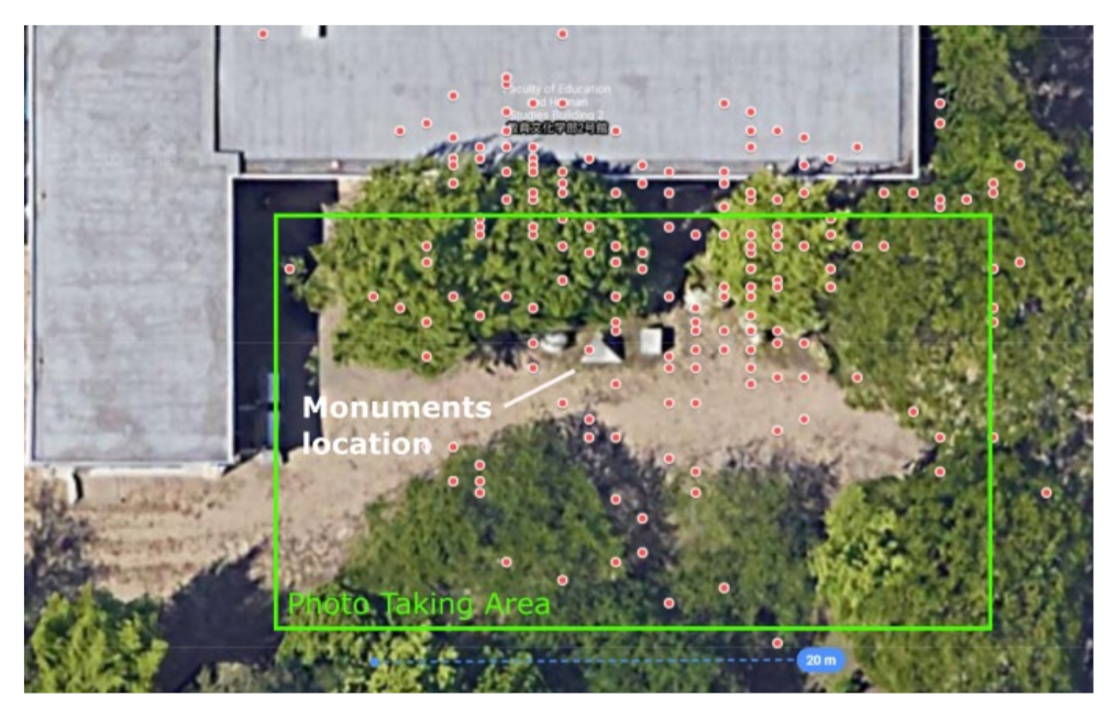
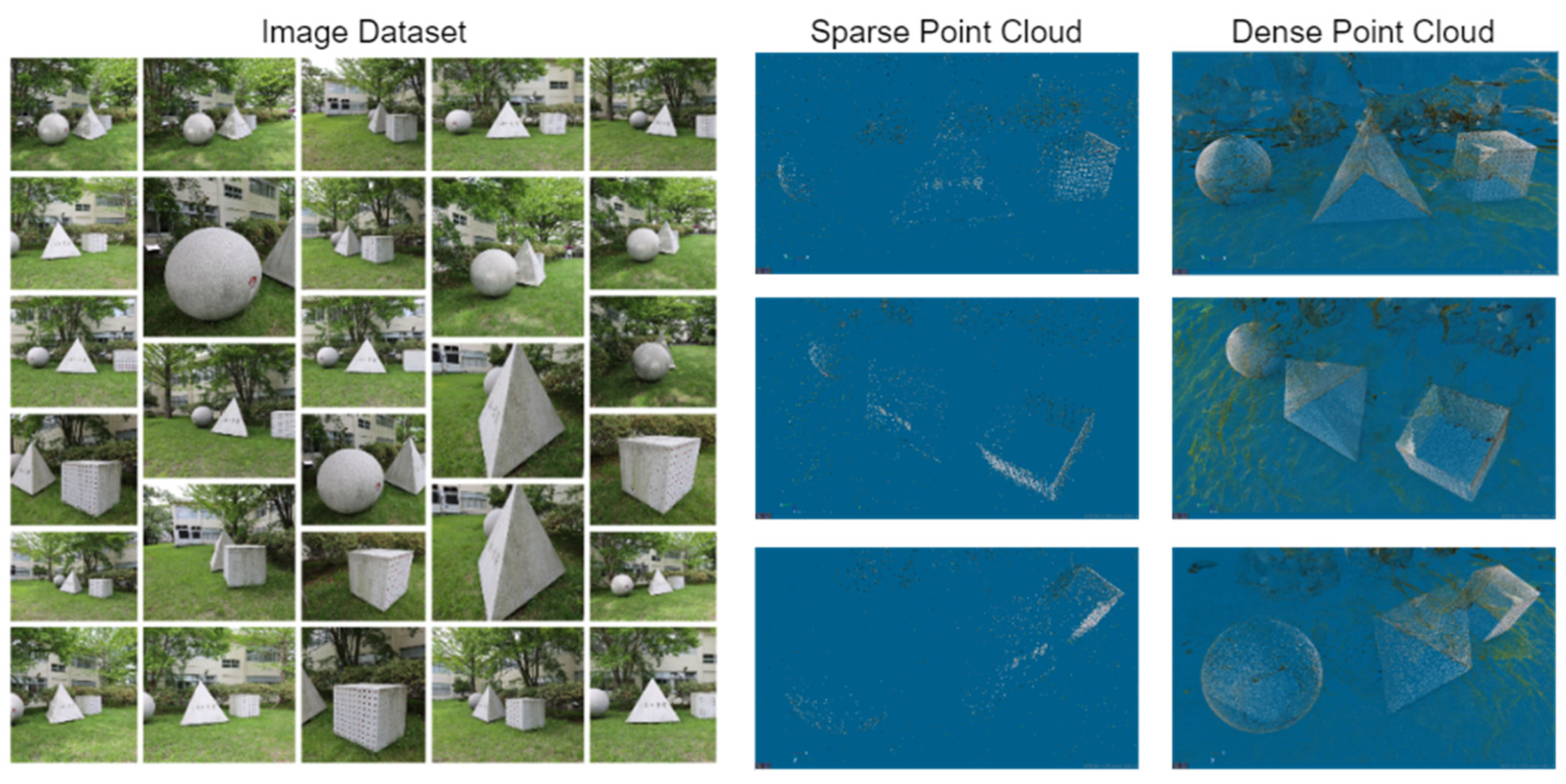
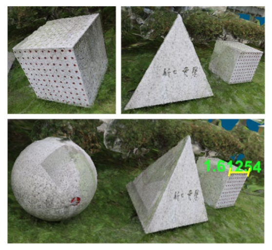
To perform quantitative evaluation of the effects of GNSS constraints on the scaling error of 3D reconstruction using SfM, an analysis using monuments of known dimensions outside Akita University was done. The experiment aims to correlate the scaling error to the number of images used in SfM. The hypothesis of this experiment is that, as more images are used, the scaling error due to GNSS error will decrease. In this scene, the cube-shaped monument has sides measuring approximately 1 m. This dimension is used to compute the scaling error. This particular scene was chosen for this reason, in addition to the monuments being of simple 3D shapes, making analysis of measurements more accurate for the purpose of quantitative evaluation.

For this experiment, around 200 images of the scene were taken across 2 days at roughly the same time of the day, with sample images shown in Figure 12 and a map of the depicted photo taking area and the recorded camera positions in Figure 13. For this and the proceeding experiment, the camera was used freehanded without a tripod, with a Xiaomi Mi 9T Pro smartphone placed close to the camera sending GNSS data to it via Bluetooth. The dataset, as with the previous experiment, was used to create 3D reconstructions at different image numbers, with an example shown in Figure 14. The scaling error when varying number of images are used was noted and compared. For reconstruction purposes in this and the following experiments, 3DF Zephyr was used, with a setting of 50% GNSS data weight, as specified in the software’s manual [22].

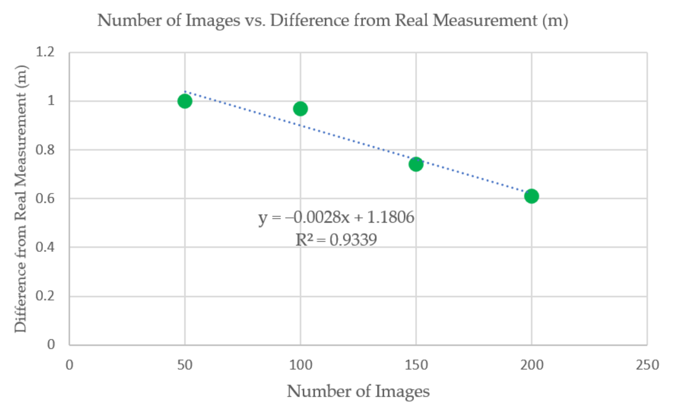
As shown in

Table 1. Results of the experiment on monuments of known dimensions.

Data	Measured (m)	Real Measurement (m)	Difference from Real Measurement (m)
50 images	2.00	1	1.00
100 images	1.97	1	0.97
150 images	1.74	1	0.74
200 images	1.61	1	0.61

and Figure 15, there is a trend that at increasing number of images used in reconstruction, the difference from the real measurement decreases. This increase in accuracy lends credence to the hypothesis that using more images for reconstruction has the tendency to lessen scale error in 3D models. Using the trendline of the data, a model with a difference from real measurement of 0.1 m (10% scaling error) can be hypothetically created if 386 (385.93) images are used.

4. Experiment on a Pseudo-Muckpile

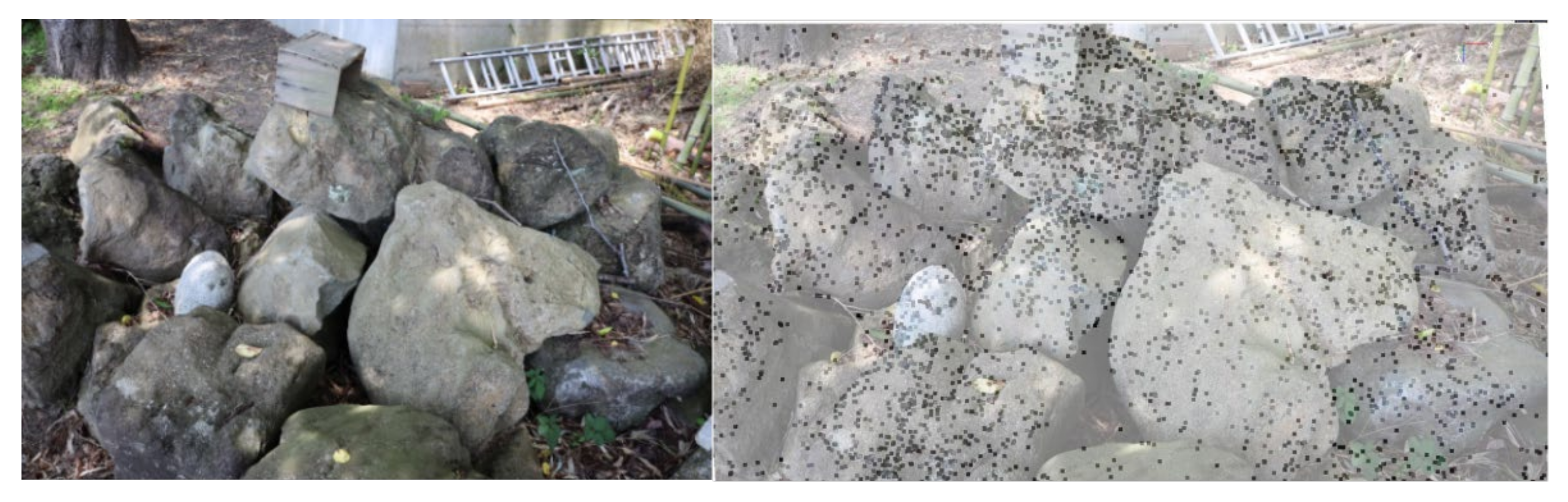
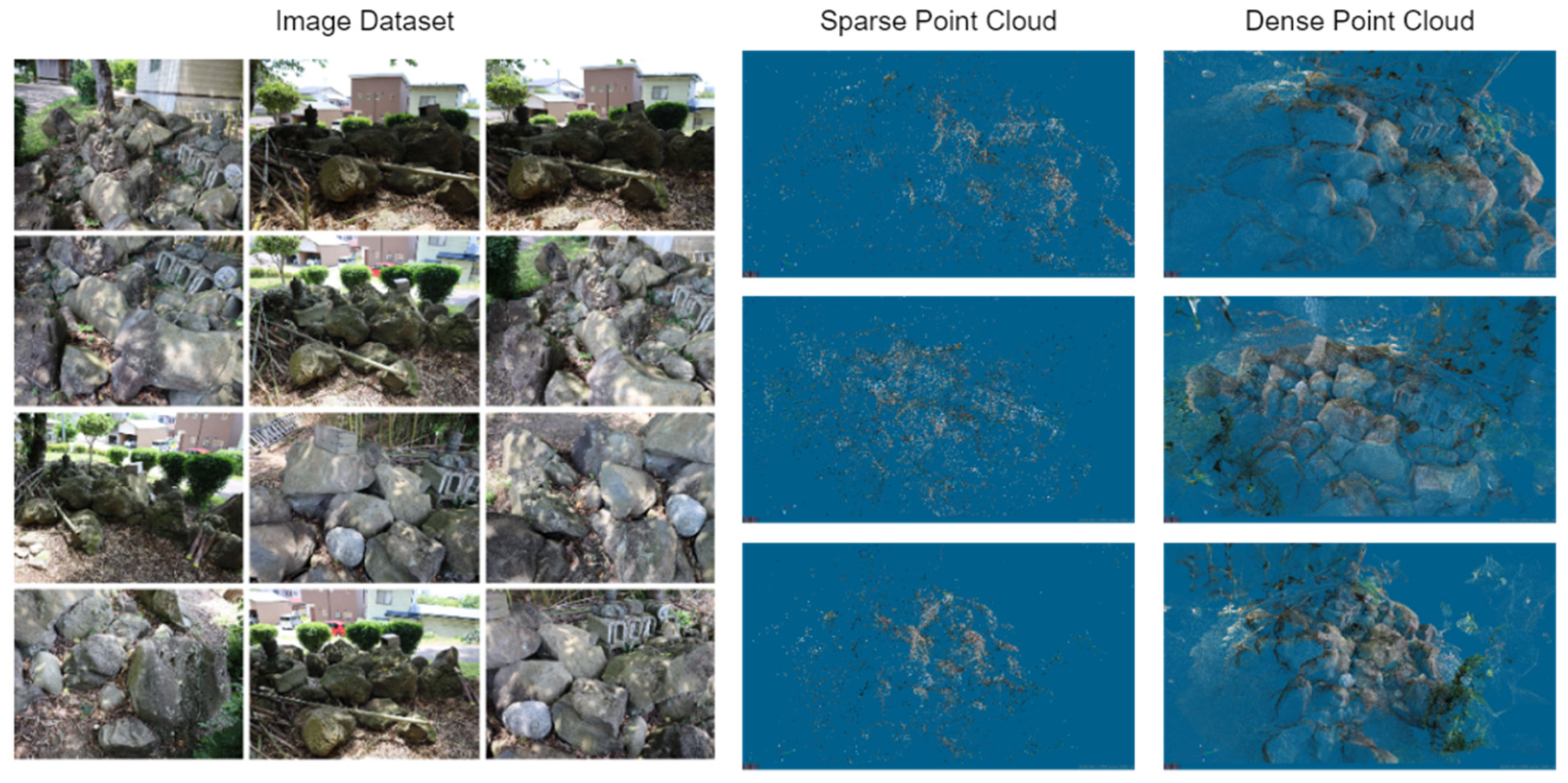
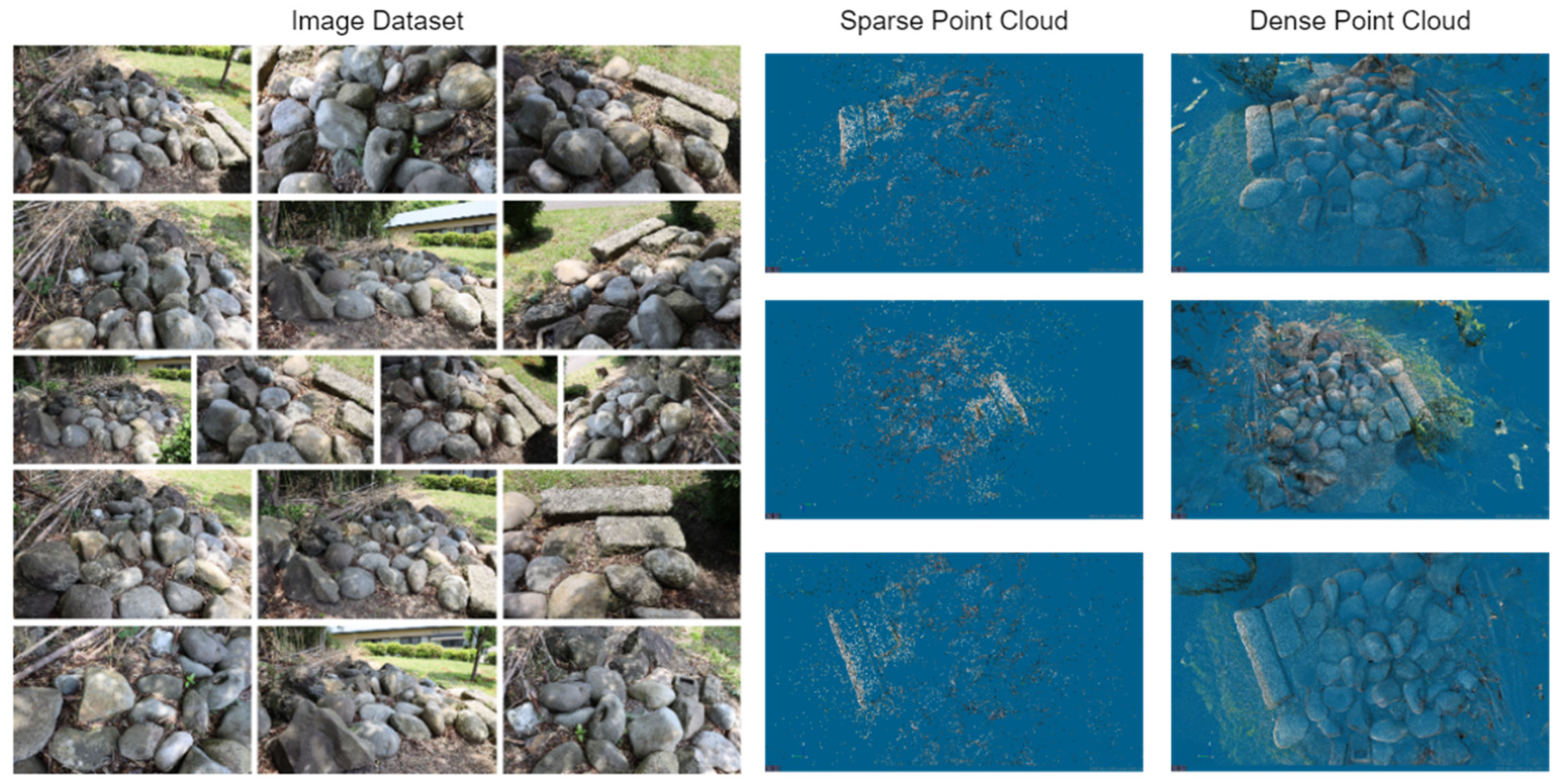
For this test, the goal was to recreate a scene of a collection of boulder-sized rocks found at a temple site near the university, shown in Figure 16. The aim of this case study is to provide both quantitative and qualitative evaluation of the effects of GNSS constraints on the scaling error of 3D reconstruction with a subject that is a close simulation of an actual muckpile in a mining environment. The study conducted an experiment using a rock pile located near Akita University. These rocks are similar in size and shape to a muckpile, and, if the effectiveness of the method on this dataset can be confirmed, it can be assumed that the method will be equally effective on an actual muckpile in a mine site.

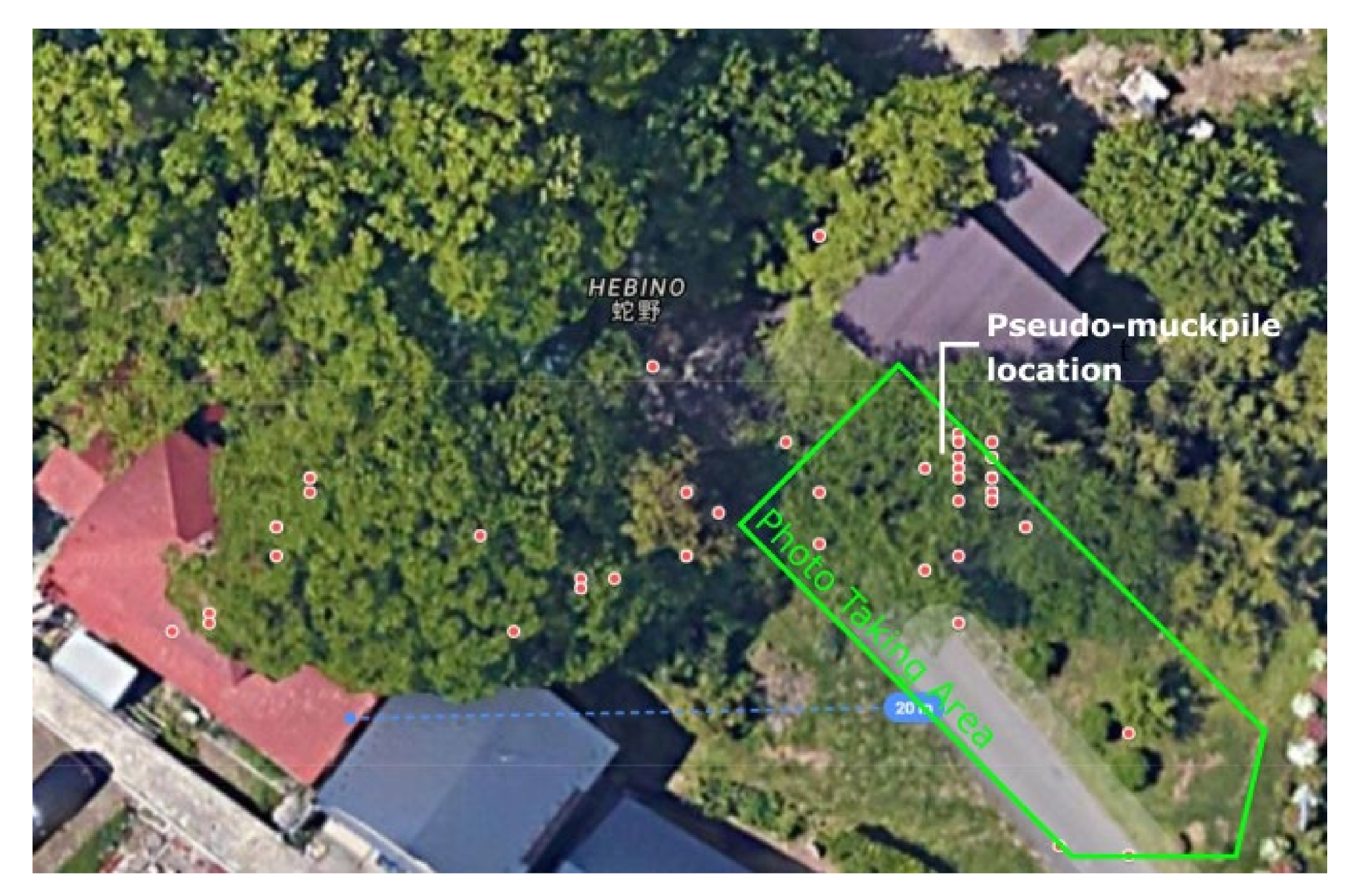
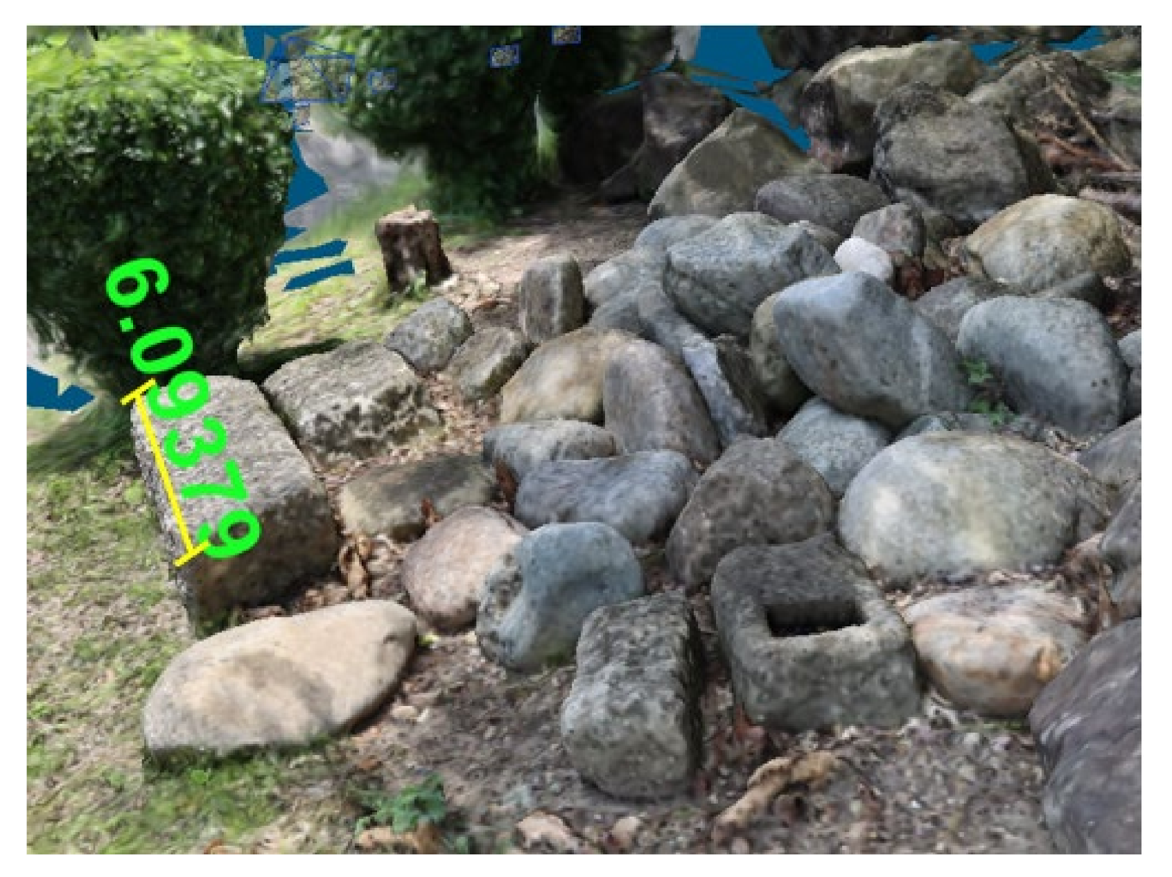
A total of 200 photos were taken and split into two datasets (Set #1 and #2) as shown in Figure 16 and Figure 17, with a map depicting the photo taking area and the recorded camera positions found in Figure 18 The rockpile was divided into two parts, one with bigger, angular rocks and another with smaller, rounded rocks. Both piles were around 4 m wide on their longest side and are less than a meter long. 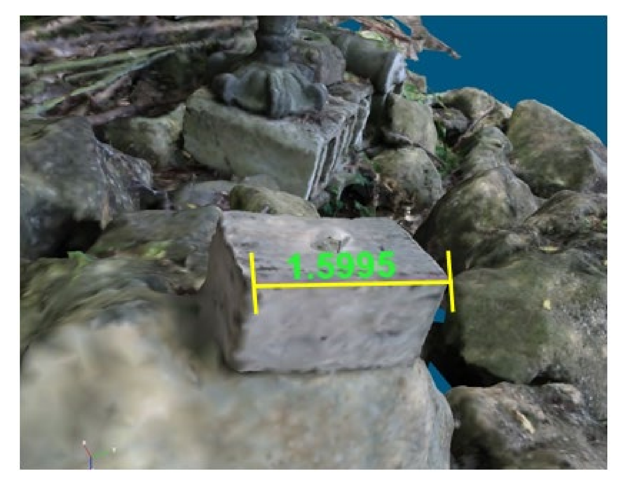A wooden box measuring 30 by 30 by 17 cm was placed in the scene for reference, as shown in its reconstructed form in Figure 19. In addition, measurement of the big, rectangular prism-shaped rock with dimensions of 35 cm × 40 cm × 30 cm were taken for reference as well, which can be seen in its reconstructed form in Figure 20.

After the photos were taken, they were once more processed to produce several 3D models at different image numbers. The scaling error and the reconstruction quality was then observed in a similar fashion to the previous experiments. Since two sets of data were used for this experiment, scaling errors between using 50 images (chosen at random) and 100 images for each set were used. An additional exploratory test using 200 images using both sets was added for testing. The study’s initial hypothesis, however, was that this will introduce some reconstruction errors as there are not enough images that are similar between these two scenes.

The measurement comparison is shown in

Table 2. Results of the experiment on a pseudo-muckpile.

Data Set and Image Count	Measured (m)	Real Measurement (m)	Difference from Real Measurement (m)
Set #1 (50 images)	2.98	0.30	2.68
Set #1 (100 images)	1.60	0.30	1.30
Set #2 (50 images)	6.11	1.40	4.71
Set #2 (100 images)	6.09	1.40	4.69
Combined Set (200 images)	0.16	0.17	0.01

. For Set #1, at 50 images used, the difference from the real measurement of the width of the box (0.3 m) was 2.6 m. At 100 images used, the difference was 1.3 m. This led to a decrease of 1.3 m in the scaling error when using 50 more images. For Set #2, at 50 images used, the difference from the real measurement of the width of the rectangular rock (1.4) was 4.8 m. At 100 images used, the difference was 4.6 m. This led to a decrease of 0.2 m in the scaling error when using 50 more images.

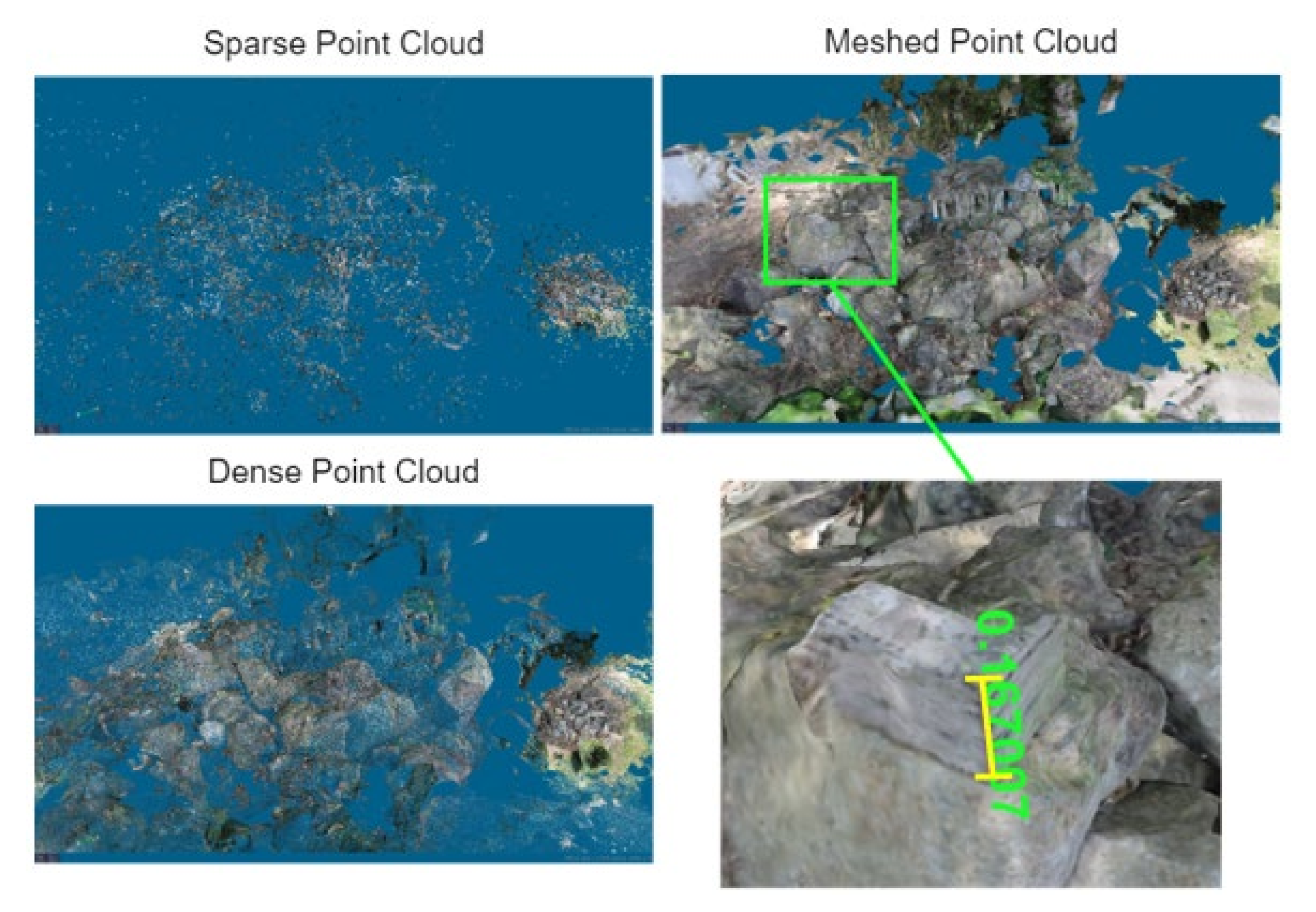
For a final, investigational set using 200 images combining both previous sets, a surprising result was observed—even though there were significantly more reconstruction errors (missing parts, duplicating parts, etc.) in this particular reconstruction, the wooden box width in this reconstruction was measured at 0.167 m with a difference of 0.01 m from the real measurement. A reconstruction is shown below in Figure 21. We considered that this increase in accuracy can be attributed to not only the number of images increasing but also the general area of the scene becoming larger as it includes both pseudo-muckpiles (the effect of model size on GNSS error is discussed in a latter part of this section). However, combining the datasets also means that the scene being reconstructed is contextually different as it now includes both parts of the pseudo-muckpile.

From both experiments, we can see through the maps in Figure 14 and Figure 17 the apparent GNSS drift that occurs during the photo taking. Some of the recorded camera positions are either outside the photo taking area or are in spots that are obstructed. The study recognizes that these changing boundary conditions have an effect on the results, and a separate investigation on this could provide insight for GNSS-aided photogrammetry. Aside from the inaccuracies found in GNSS, several additional factors have been considered to contribute to the drift. One of these is the effect of the partial tree cover in some of the camera positions.

A previous study [23] in a similar setting (university campus) analyzed the effect of not only partial tree cover but also nearby infrastructure on GNSS accuracy by comparing GNSS data to total station survey data. The results showed that some points were no longer suitable for GNSS positioning due to high GDOP (geometric dilution of precision), and, where it was suitable, the GNSS recorded position differed by as much as 5.7 m from the total station data. This difference is consistent with what transpired in this study’s experiments, as can be seen from the maps. In a mining site, where there is usually less vegetation and obstruction, this effect should be diminished, except in situations such as benches shadowing satellites.

Another factor that can be considered is the overall scale of the pseudo-muckpile. A large majority of GNSS-aided photogrammetry applications are typically in the form of aerial imagery and mapping with a scope and scale larger than both of the terrestrial photogrammetry experiments performed in this study. A study [24] investigating the application of terrestrial photogrammetry in field geology by using SfM-MVS aided by GPS to model an outcrop that long observed scaling and rotational errors in their reconstruction. Aside from concluding that GNSS contributed highly to these model errors, they suggested that, at a larger scale, the error would be less of an issue.

In parallel to this, the study observed that the relatively small scale of the experiment area affected the data; particularly the pseudo-muckpile whose size was smaller than a muckpile that one would normally find in a mining operation. Ultimately however, the results showed that, even at this scale, incremental improvements to 3D model scaling have been made as shown in the data.

5. Conclusions

In this paper, we proposed a low-cost method of creating an accurately scaled 3D model without the use of GCPs by constraining camera positions through the use of georeferenced images as input for SfM. Monitoring fragmentation size is an important procedure in optimizing mining operations that perform blasting. In recent years, a new method that involves using 3D photogrammetry to measure fragment sizes has been developed and has the potential to surpass traditional techniques. For this particular process to be accurate, a method for properly scaling 3D model with georeferenced images using GNSS was investigated.

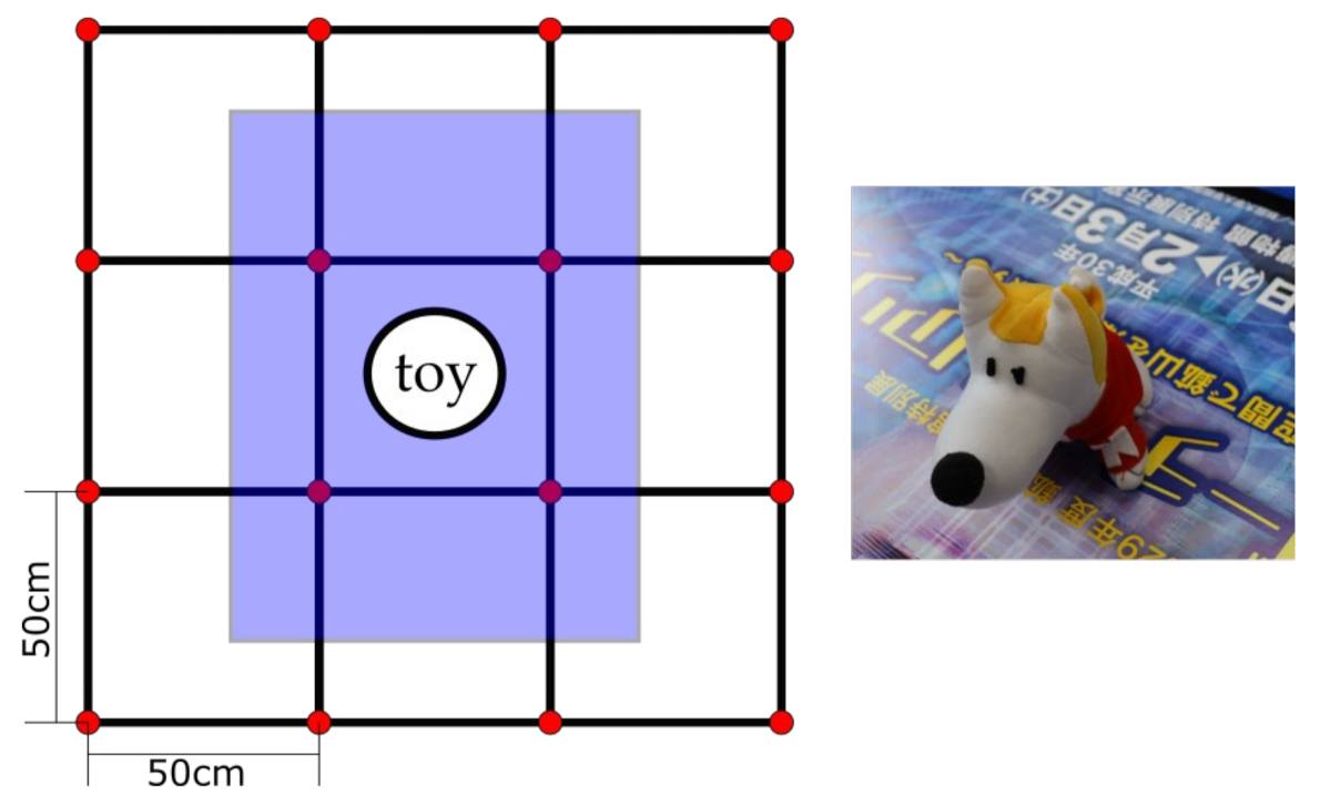
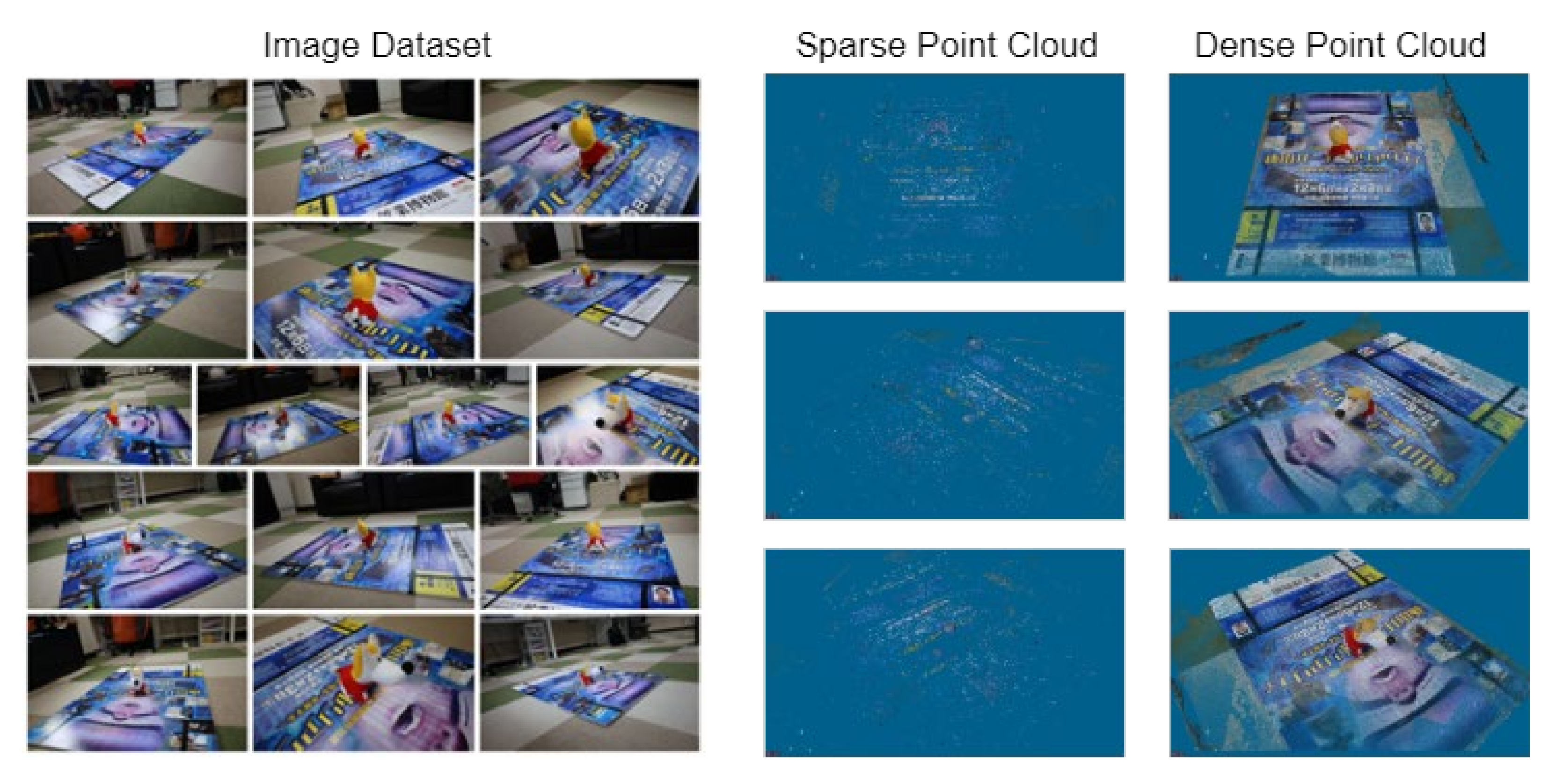
To validate the method, several experiments were performed. As an initial test to prove the fundamentals, an indoor scene involving a small object was recreated in 3D space using SfM with photos of the known relative positions for constraining the camera location, and good results that showed that the created 3D model had a scaling error of 1.27 cm were achieved. For the main experiment, the study took georeferenced photos of an outdoor scene with a monument of known dimensions and made several reconstructions at increasing number of images used (50, 100, 150, and 200 images, respectively). The results showed a linear pattern with an R-squared value of 0.93 in which the scaling error decreases as the number of images used increased.

Finally, an experiment was performed to verify the study’s hypothesis further using a scene that included a pseudo-muckpile to simulate the usage of the proposed system for a mining operation. In a similar fashion, the results showed increasing scale accuracy with an increasing number of images used in reconstructions. Two observations can be drawn from the experimental results: (1) constraining cameras to accurate positions in SfM resulted in a properly scaled 3D model and (2) increasing the number of georeferenced images in SfM incrementally improved the scaling error of the reconstruction. These observations can help improve scale accuracy in GNSS-aided 3D fragmentation measurements. The method described in this study will be of interest when cost-efficiency and practicality are desired in a 3D fragmentation measurement system.