Determination of Trace Metal (Mn, Fe, Ni, Cu, Zn, Co, Cd and Pb) Concentrations in Seawater Using Single Quadrupole ICP-MS: A Comparison between Offline and Online Preconcentration Setups

Abstract

The quantification of dissolved metals in seawater requires pre-treatment before the measurement can be done, posing a risk of contamination, and requiring a time-consuming procedure. Despite the development of automated preconcentration units and sophisticated instruments, the entire process often introduces inaccuracies in quantification, especially for low-metal seawaters. This study presents a robust method for measuring dissolved metals from seawater accurately and precisely using a seaFAST and quadrupole Inductively Coupled Plasma Mass Spectrometer (ICPMS), employed in both offline (2016–2018) and online (2020–2021) setups. The proposed method shows data processing, including the re-calculation of metals after eliminating the instrumental signals caused by polyatomic interferences. Here, we report the blank concentration of Fe below 0.02 nmol kg⁻¹, somewhat lower values than that have been previously reported using high-resolution and triple-quad ICPMS. The method allows for the accurate determination of Cd and Fe concentrations in low-metal seawaters, such as GEOTRACES GSP, using a cost-effective quadrupole ICPMS (Cd_consensus: 2 ± 2 pmol kg⁻¹, Cd_measured: 0.99 ± 0.35 pmol kg⁻¹; Fe_consensus: 0.16 ± 0.05 nmol kg⁻¹, Fe_measured: 0.21 ± 0.03 nmol kg⁻¹). Between two setups, online yields marginally lower blank values for metals based on short-term analysis. However, the limit of detection is comparable between the two, supporting optimal instrumental sensitivity of the ICPMS over 4+ years of analysis.

1. Introduction

The sources, cycling, and fluxes of trace elements in seawater have become a prime interest in understanding ocean life and the interaction between ocean and atmosphere. The role of trace elements in the global ocean widely varies based on their involvement in oceanic processes, starting from the primary production of phytoplankton to assessing anthropogenic contributions. Using trace elements as tracers, e.g., Fe, Mn, Cu, Zn, Ni, Co, and Cd as bio-essential metals for productivity, Fe and Mn for hydrothermal/riverine input, Mo for redox processes, Pb for anthropogenic activities, Al for natural dust input, and Nd for mixing of water masses, has provided new insights regarding our understanding of the ocean [1]. Therefore, the GEOTRACES and its precursor programs (e.g., JGOFS, WOCE), enabled the construction of a spatiotemporal database of trace elements and their isotope (TEIs) within the global ocean. However, analytical processes for generating TEIs data, especially for particulate and dissolved metals, contain challenges. The extremely low concentration of metals, sea salt-derived interferences, and the risk of contamination could limit the analytical accuracies. Thus, scientists devised methods to purify (remove sea salts) and preconcentrate seawater before analysis. The pre-processing of the samples has been improved by applying different methodologies (e.g., solvent extraction, magnesium hydroxide co-precipitation, solid-phase extraction) [2,3,4]. In addition, technological advancements have facilitated the quantification procedure accurately and precisely by utilizing sophisticated analytical techniques (e.g., flow injection, cathodic stripping, atomic absorption, mass spectrometry; [5,6,7,8]). In particular, a commercially available automated module, the seaFAST system, simplifies and streamlines the pre-processing treatment of seawater samples. Several studies have shown the potential of using the seaFAST pre-treatment system before quantifying trace metals [9,10,11,12,13], rare earth elements [14,15], and their isotopic composition [16]. Once preconcentrated, the advanced, high-resolution mass spectrometers, e.g., sector field (SF-ICPMS; [9]) and triple quadrupole (QQQ-ICPMS; [10]) have been commonly used for quantification. In some studies, a single quadrupole ICPMS was also applied for the determination of trace metals [12,17].

The seaFAST comprises a column packed with chelating resin that effectively removes sea salts and then elutes preconcentrated trace elements. Although the preconcentration factor may reach up to 50 times and more, quantifying selective bio-essential metals (e.g., Fe, Zn, Cd), often requires high mass resolution in the ICPMS to distinguish the analytes from instrumental backgrounds [10,11]. However, adding a collision reaction cell (CRC) to the ICP-MS instrument minimizes the instrumental background by dissociating polyatomic interferences [18]. To further optimise the analytical setup, the seaFAST module may be coupled directly to the ICPMS, i.e., online (e.g., [12]), which reduces preparation time and intermediate steps between preconcentration and quantification involved in the offline method.

The development of offline and online systems improved and simplified the methodology by simultaneous quantification of multiple analytes for a large number of seawater samples. However, measuring selective bio-essential and contamination-prone metals (e.g., Fe, Zn, Pb, Cd) often introduces inaccuracies that stem from potential contaminant contributions from the various steps in the analytical process (e.g., reagents, tubing) used in the seaFAST and/or higher background signals caused by polyatomic interferences on specific metals. For example, it was estimated that argon oxide (ArO⁺), derived from the argon gas used to produce the plasma, contributed 60%–85% of the measured ⁵⁶Fe_blank concentration [10]. The contribution of masses from both contamination and polyatomic interferences could increase the limit of detection for metals thereby preventing the measurement of selected analytes (e.g., Cd, Fe, Zn) which are characterised by extremely low concentrations in surface seawater. In addition, measurement can be erroneous because of the high proportional contribution of added mass. Therefore, the measured concentration is generally subtracted by the instrumental counts of procedural blanks [9]. For Cd, Cd-free seawater or molybdenum (Mo)-standard is analysed to quantify the magnitude of molybdenum oxide (MoO⁺) derived Cd, i.e., up to 9 pmol kg⁻¹ [9]. However, we have limited knowledge on the following: (1) the degree of proportional contribution of added mass for a range of analyte concentration, (2) the requirement of blank subtraction to obtain the actual concentration of metals in seawater, (3) polyatomic interference and its effect on different isotopes of an analyte, and (4) selection of isotopic mass that produces the least interference.

Based on our experiments carried out in the previous five years, using both offline and online, we present a robust methodology that allows accurate and precise measurement of dissolved metals (Mn, Fe, Co, Ni, Cu, Zn, Cd, and Pb) using a single Q-ICPMS. The proposed methodology includes both measurement and post-processing calculation of data. The results of selected metals measured using offline setup are already published [19,20,21]. In this manuscript, we focus mainly on the effect and magnitude of polyatomic interferences, especially while measuring Fe and Cd, and present our findings to assess the magnitude and degree of interference needing to be corrected. In addition, the results from this study offer a comparison between offline and online method setups and support using cost-effective single Q-ICPMS (compared to High Resolution-, SF-, and QQQ-ICPMS) for quantifying dissolved trace metals from seawater.

2. Analytical Methods

2.1. Reagents and Materials

High-quality deionized water (DIW; 18.2 M-Ω resistivity) was produced using the Milli-Q^® advantage A10^® system (MilliporeSigma, Burlington, MA, USA), fitted with a Q-POD^® Element dispenser as an added trace contaminant removal device, and used throughout the analytical procedures and preparations thereof. For use during the preconcentration procedure (Section 2.2), an ammonium acetate buffer (pH: 6.0 ± 0.2) was prepared by mixing 25% ammonium hydroxide (NH₄OH; Merck Suprapur^®, Darmstadt, Germany), 100% glacial acetic acid (CH₃COOH; Merck Suprapur^®), and DIW. The pH of the buffer solution was read using a pH electrode (Hach^® sensION^TM PH1, resolution of ±0.01). The elution acid comprised 5% M nitric acid (HNO₃; Merck Ultrapur). All solutions were prepared inside a fume hood housed within a class 100 clean laboratory (TracEx lab, Stellenbosch University, Stellenbosch, South Africa). All plasticware, containers, and sample bottles used for the storage of seawater and reagents were extensively acid cleaned according to strict protocols outlined by GEOTRACES [22]. The material of the lab wares (e.g., reagent bottles, measuring cylinder, vials, and pipette tips) was either polypropylene/ethylene (PP/PE) or Perfluoroalkoxy alkanes (PFA) and used after thorough acid cleaning.

2.2. Automated Preconcentration Using seaFAST Module

Both offline (period of use: 2016–2018) and online (period of use: 2020–2021) variations of the method utilised a solid phase extraction (SPE) technique to separate the trace metal ions from the seawater matrix elements. A SC-4 DX seaFAST-pico module (Elemental Scientific Inc; ESI, Omaha, NE, USA) was used for the offline preconcentration of samples, while the SC-4 DX seaFAST S3 (ESI) was used for the online variation of the method (

Table 1. Offline and online preconcentration setup.

Mode of Analysis	Offline	Online
Preconcentration module	SC-4 DX seaFAST-pico	SC-4 DX seaFAST S3
Column resin	Nobias (EDTriA and IDA)	Nobias (EDTriA and IDA)
Sample pH	1.7	1.7
Buffer	Ammonium acetate (pH: 6.0 ± 0.2)	Ammonium acetate (pH: 6.0 ± 0.2)
Eluent	5% HNO3	5% HNO3
Internal Standard	-	10 µg kg−1 In
Sample loop (mL)	10	3
Elution cycles	4	1
Elution volume (mL)	0.25	0.1
Preconcentration factor	40	30
Sample throughput (min sample−1)	20	11

). The SC-4 DX seaFAST S3 has a hood with a built-in high-efficiency particulate air (HEPA) filter, which encloses the autosampler allowing the module to be used outside the clean lab (Figure S1). The SC-4 DX seaFAST-pico does not come standard with a HEPA hood, and therefore, the module was kept in a class 100 clean lab. As an added precaution against sample contamination from falling particulate, we manufactured a perspex hood to fit over the autosampler and sample rack. Both modules are commercially available and consist of an autosampler, a syringe module (S400V), a sample loop (10 mL for seaFAST pico and 3 mL for the seaFAST S3), two 11-port valves (A11b and P11), one 5-port valve (A5e), one trace metal clean-up column (CF-N-0200 for seaFAST S3 and CF-M-0600 for seaFAST pico; 200 µL bed volume) and a preconcentration column (CF-N-0200; 200 µL bed volume). Both modules were pressurized using clean air (99.999% O₂; Air Products). The autosampler, with an inner probe diameter of 1 mm, introduced samples from the sample rack into the preconcentration manifold via a vacuum pump system. The S400V syringe pump controlled the four syringes (S1, S2, S3, and S4), which were dedicated to reagent distribution while their flow path was controlled by the FAST DX 3 valve module. Syringe S1 (DIW) consists of a 12 mL barrel with a dispense rate of 500 µL min⁻¹, while the other syringes (S2: Buffer; S3: Eluent/Carrier; S4: Eluent/Diluent/Internal Standard) comprised a 3 mL syringe with a dispense rate of 496 µL min⁻¹. Once introduced, the sample was loaded through the 5-port valve by vacuum pressure and then transferred to the sample loop connected to the A11b valve. Since the A11b valve switches, the sample is pushed to the P11 valve and mixed with the buffer solution, before transferring to the seawater preconcentration column (See Supplementary Section Figure S1). The preconcentration resin comprised both ethylenediaminetriacetic acid (EDTriA) and iminodiacetic acid (IDA) functional groups immobilized on a hydrophilic methacrylate polymer (60 µm bead diameter). As the buffered seawater passes through the column, the dissolved trace metals are chelated by the resin, while the seawater matrix is washed out from the column. The eluent is then driven through the preconcentration column, thereby eluting the trace metal ions. For offline preconcentration, the chelated metal ions were eluted into acid cleaned PP Falcon™ tubes during 4 elution cycles for a final elution volume of 0.25 mL, achieving a preconcentration factor of 40 and a sample throughput of 20 min/sample. For online preconcentration, the chelated metal ions were eluted directly into the nebuliser of the ICP-MS instrument after 1 elution cycle for a final volume of 0.1 mL, a preconcentration factor of 30, and a sample throughput of 11 min/sample. The elution is followed by cleaning and condition by a mixture of buffer and DIW in preparation for the next sample. After each sample, the probe was rinsed in a 2% HNO₃ (Ultrapur, Merck) solution followed by DIW.

2.3. ICP-MS

Sample analysis of preconcentrated samples was performed on an Agilent 7900 quadrupole Inductively Coupled Plasma Mass Spectrometer (ICP-MS) (Agilent Technologies, Santa Clara, CA, USA) with operating conditions outlined in

Table 2. ICP-MS operating parameters.

Mode of Analysis	Offline	Online
Instrument	Agilent 7900	Agilent 7900
Nebulizer	200 µL PFA	PFA-ST microflow (400 μL min−1)
Cones	Ni plated (sample and skimmer)	Ni plated (sample and skimmer)
Sensitivity	>109 cps/ppm at <2% CeO	>109 cps/ppm at <2% CeO
RF power (W)	1600	1450
Spray chamber	Double pass	Cyclonic
Torch depth (mm)	10	8
Make-up gas (L/min)	0.25	0
He gas flow (mL/min)	4.8	4.8
H2 gas flow (mL/min)	6	0
Cool gas flow (L/min	15	15
Auxiliary gas flow (L/min)	0.9	0.9
Sample gas flow (L/min)	0.95	1.07
Sample uptake (s)	18	100
Sensitivity for 1 ppb Y (cps)	45,000	32,000
Oxide ratio	<0.3%	<0.3%

. The offline method requires the eluted samples to be taken to the ICP-MS laboratory, therefore, there is a time interval between sample elution and ICP-MS analysis. The instrument was optimized for sensitivity and low oxide ratios (<0.3%). Trace metals (Mn, Fe, Ni, Cu, Zn, Co, Cd, and Pb) concentrations were measured using the Agilent Octopole Reaction System (ORS) in He collision mode. For samples preconcentrated offline, Fe was analysed in H₂ reaction mode in order to eliminate plasma-based interferences (e.g., ⁴⁰Ar¹⁶O⁺). For online preconcentrated samples, Fe was run in He collision mode like the other trace metals and the argon oxide signal from the plasma was used to correct Fe values manually.

2.3.1. Calibration

The instrument was calibrated using two different methods. For samples preconcentrated offline, a custom blend ICP-MS multi-element standard (MES) from Inorganic Ventures was used as a calibration standard. The MES contained only metals and no alkali ions and was verified by simultaneous analysis of a certified MES (IV-28; Inorganic Ventures^®). A 4-point calibration curve was constructed over a wide concentration range using: 0, 1, 10, and 20 µg kg⁻¹ concentrations. The linearity of the calibration was decided ensuring that 40 times preconcentrated trace elements fall within the range. The MES was prepared in 2% HNO₃ (Ultrapur, Merck).

For samples preconcentrated online, the instrument was calibrated using three dilutions of the calibration standard (STD1, STD2, and STD3) and the diluent (surface seawater; STD0). Given that the concentration of dissolved metals (bio-reactive) is minimum in surface seawater, we used it as a diluent to ensure the measured concentrations fall within the linearity of calibration. The calibration standards were made as per Equations (1)–(3). We particularly used the serial dilution technique, where STD3 (high concentration) was used to prepare STD2 (mid-concentration), and STD2 was further diluted to STD1 (low concentration).

$$C_{STD3}=C_M\times \frac{m_M}{m_M+m_{STD0\left(i\right)}}$$

(1)

$$C_{STD2}=C_{STD3}\times \frac{m_{STD3}}{m_{STD3}+m_{STD0\left(i+1\right)}}$$

(2)

$$C_{STD1}=C_{STD2}\times \frac{m_{STD2}}{m_{STD2}+m_{STDo\left(i+2\right)}}$$

(3)

where C is the concentration, m is the mass, M is the stock solution (Inorganic ventures^® SEP-445), and I is the dilution step.

The linearity of calibration varies among analytes based on their concentration in the surface seawater used as a diluent. For example, the linearity ranged from ca. 1.4 to 242 ng kg⁻¹ for Co and Cd, ca. 7 to 600 ng kg⁻¹ for Fe, and ca.40 to 696 ng kg⁻¹ for Ni. The lowest calibration point was always higher than the limit of detection (LOD).

2.3.2. Monitoring Instrument Drift

For samples preconcentrated offline, internal standard addition for drift correction was not possible using the self-aspirating nebulizer. When the internal standard was pumped in and mixed with the sample, the resulting change in the uptake speed of the self-aspiration would induce signal instability. We used self-aspiration for the sample introduction in order to analyse all the trace elements simultaneously from the very small sample volume (0.25 mL). Manual drift correction was applied using the continuous standards measured during each analysis session. Analysis was therefore carried out in a standard sample bracketing format by running the MES calibration standard every 6 samples. Where drift exceeded 5% relative to the starting concentration of the MES for a specific element, a drift correction was applied using Equation (4).

$$2\times \frac{Con{c}_{MES\_start}}{\left(Con{c}_{ME{S}_{\_a}}+Con{c}_{MES\_b}\right)}\times Con{c}_{sample}$$

(4)

where a and b are the MES before and after each set of 6 samples. The instrument was re-calibrated if the drift exceeded 20% or after 3 h of instrument run time. To reduce contamination risk, preconcentrated samples were manually opened ±5 s prior to each sample introduction.

For samples preconcentrated online, Indium (In) was monitored throughout the analyses as an internal standard to track instrumental drift with time. A single internal standard was used in order to minimise the risk of contamination, and In was chosen as it does not suffer from or produce any matrix interferences on the analytes of interest, while its position on the periodic table places it within the mass range of the analytes (⁵⁵Mn to ²⁰⁸Pb) to be appropriate for drift correction.

The In-normalized analytical signal was processed to calculate the calibration slopes (S) and final concentrations. A typical operational sequence begins with a calibration, which is then followed by a set of unknown samples (reference standards, unknown seawater, procedural blank) and ends with another calibration. We performed several consecutive sequences in a single instrument run. The calibration slope of analyte j (nth calibration) can be estimated:

$$S_j^n=\frac{(STD{3}_j:STD{0}_j)}{\left(\frac{signa{l}_{STD3-j}}{signa{l}_{STD3-IS}}:\frac{signa{l}_{STD0-j}}{signa{l}_{STD0-IS}}\right)}$$

(5)

The measured concentration of analyte j for an unknown sample (US) was calculated based on a standard bracketing method.

$$C_j^{US} =\frac{signa{l}_{US-j}}{signa{l}_{US-IS}}\times Avg \left(S_j^n:S_j^{n+1}\right)$$

(6)

The blank corrected concentration of seawater (SW) was finally determined following Equation (7).

$$corrected C_j^{SW}=C_j^{SW}-C_j^{procedural blank}$$

(7)

2.4. Procedural Blanks and Limit of Detection (LOD)

The procedural blank incorporates the potential contribution of the reagents, materials, instrument manifolds, and arbitrary incidents, to the field sample. For the offline method, the procedural blank was quantified during a single instrument run (short-term) by preconcentrating a solution of 2% HNO₃ (n = 5) using the same analytical technique employed for field samples. For the online method, the procedural blank was quantified by preconcentrating 1% HCl, where we monitored both short-term (n = 7, based on a single instrument run) and long-term (n = 77, combination of 13 separate instrument runs) blank values. In both cases, the LOD was calculated according to Equation (8).

$${\mathrm{LOD}}_j=3{\sigma }_{procedural blank}$$

(8)

For the online preconcentrated samples, a second approach, based on the calibration curve of each element, was also used to calculate the LOD (Equation (9))

$${\mathrm{LOD}}_j=\frac{3{\sigma }_{cal}}{S}$$

(9)

where σ_cal represents the standard deviation associated with the y-intercept and S is the calibration slope.

2.5. Reference Materials—NASS-7 and GEOTRACES (GSP and GSC)

The NASS-7 (National Research Council, Ottawa, ON, Canada) certified reference material (CRM) as well as two GEOTRACES reference materials representing low (GSP-62) and high (GSC 1–19) trace metal concentration ocean water were analysed in order to assess method accuracy. The measured trace metal concentrations were compared to respective certified and consensus values and the accuracy of each metal was calculated using Equation (10)

$$Accuracy=\left(\frac{dT{M}_{measured }-dT{M}_{reported}}{dT{M}_{reported}}\right)\times 100$$

(10)

2.6. Recovery

For samples preconcentrated offline, a simple experiment was designed to test the seaFAST resin recovery. Bulk seawater representing Southern Ocean Surface Waters (SOSW; 55° S; 28° E) was spiked with a 200 ng kg⁻¹ multi-element standard (MES). The initial trace metal concentrations of the SOSW were determined by replicate analysis (n = 10) in conjunction with the NASS-7 and GEOTRACES reference seawater. For samples preconcentrated online, a similar experiment was carried out. Bulk seawater, also representing Southern Ocean surface waters but from a different location (38° S; 11° E), was spiked with a MES. The MES contained 161 ng kg⁻¹ for all trace metals except Co and Cd (65 ng kg⁻¹). The initial trace metal concentrations of the SOSW were also determined by replicate analysis (n = 10) in conjunction with the NASS-7 and GEOTRACES reference seawater. In both experiments, the initial trace metal concentrations were subtracted from the SOSW + spike concentrations in order to quantify the recovery as a percentage of the spike concentration.

2.7. Quantifying Polyatomic Interferences

During ICP-MS analysis, polyatomic interferences on trace metal signals, particularly isotopes of Fe and Cd, can lead to inaccurate quantification. For ⁵⁶Fe, argon oxide is the most pertinent interference (

Table 3. Potential polyatomic interferences on Fe and Cd isotopes.

Isotope	Interference
56Fe	40Ar16O+
110Cd	94Mo16O+; 110Pd
111Cd	95Mo16O+; 94Zr16O1H+
112Cd	96Mo16O+; 40Ar216O2+; 96Ru16O+; 112Sn+
114Cd	98Mo16O+; 98Ru16O+; 114Sn+

). For Cd, a host of interferences including argon and molybdenum (Mo) oxides, other trace metals such as zirconium (Zr) and ruthenium (Ru) as well as palladium (Pd) and tin (Sn) isobaric interferences can influence the various isotopic signals of Cd (Table 3). In order to understand the polyatomic interferences on the instrument signals, we monitored multiple atomic masses for Fe and Cd and compared the resulting isotopic ratios to the natural isotopic abundance.

Due to the ICP-MS plasma being produced by ionizing Ar gas (Ar⁺ + e⁻), the formation of argon oxides is difficult to circumvent. The contribution of ⁴⁰Ar¹⁶O⁺ and ⁴⁰Ar₂¹⁶O₂⁺ to the procedural blanks of ⁵⁶Fe and ¹¹²Cd respectively were therefore determined by monitoring the instrumental signal of ⁵⁶Fe/⁵⁷Fe and ¹¹¹Cd/¹¹²Cd without introducing samples into the ICP-MS (i.e., isotopic signals derived only from the plasma).

The Mo concentration in seawater is ubiquitously high (~100 nmol kg⁻¹), compared to the picomolar concentration range of Cd, and results in Mo oxide interferences on numerous Cd isotopes. Therefore, Cd-free Mo solutions were analysed over a range of Mo concentrations in order to quantify any Cd production (from Mo oxides) and correct the measured Cd concentrations, especially for low-Cd seawaters. The Pd, Zr, Ru, and Sn-based interferences on Cd are not dealt with further in this manuscript owing to (1) their low picomolar concentrations in seawater [23,24,25,26]; (2) their low natural isotopic abundances: ¹¹⁰Pd (12%); ⁹⁴Zr (17%); ⁹⁶Ru (6%); ⁹⁸Ru (2%); ¹¹²Sn (1%) and ¹¹⁴Sn (1%) and (3) robust instrument conditions and the use of CRC within the ICP-MS to eliminate oxide-based interferences [27,28].

Lastly, seawater matrix elements (Na⁺, K⁺, Ca²⁺, Mg²⁺, and Cl⁻) can affect the quantification of other trace metals, e.g., ⁴⁰Ar²³Na⁺ on ⁶³Cu [3] as well as compromise ion transmission (and therefore ICP-MS instrument sensitivity and recovery), by precipitating on the instrument cones. Matrix-based interferences were however eliminated during the preconcentration step whereby matrix ions were separated from the trace metal ions and discarded.

2.8. Data Verification

In addition to the analysis of various reference materials (Section 2.5), further steps were taken to verify the trace metal data.

2.8.1. Precision

Method precision was calculated based on sample replicates from analyses using Equation (11).

$$\% Coefficients of variation \left(CV\right)={\left[\frac{1}{2n}\times {\displaystyle \sum }{\left(\frac{\sigma }{\mu }\right)}^2\right]}^{0.5 }\times 100$$

(11)

where σ is the standard deviation between replicates, µ is the mean of replicates and n is the number of samples.

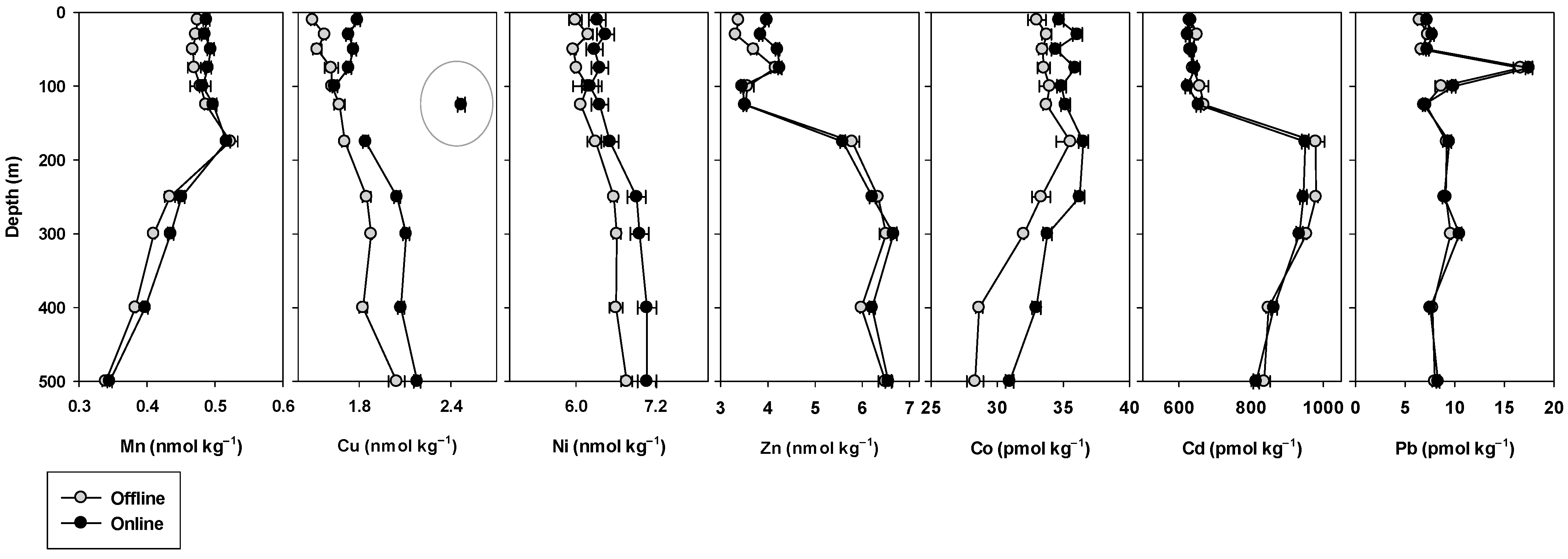
2.8.2. Crossover Station

Seawater samples were collected between surface and depth from the Southern Ocean (54° S; 0°) during the Southern Ocean Seasonal Cycle Experiment (SOSCEx) expedition in July 2015. Samples were collected along a transect between Cape Town and Antarctica using twenty-four 12 L Teflon coated GO-FLO bottles (General Oceanics) mounted on a GEOTRACES compliant CTD rosette. A vertical depth profile sampling method was executed according to GEOTRACES compliant clean protocol [22]. Directly upon recovery of the rosette, the GO-FLO bottles were transported into a class 100 clean lab for sub-sampling. Samples for dissolved trace metal determination were collected in 125 mL acid-cleaned, Nalgene™ (Thermo Scientific™) LDPE bottles after online filtration through 0.2 µm Acropak™ Capsule (Supor^® 500) filters under slight N₂ gas (99.999% N₂, BIP technology) assistance. Samples were acidified (pH = 1.7) on-board under a class 10 laminar flowhood using hydrochloric acid (HCl, Ultrapur, Merck) and stored until analysis. Samples were analysed for a suite of trace metals by both offline and online method variations and compared in order to assess analytical consistency. Method comparisons were focused on the upper water column, where trace metal concentrations are typically at their lowest and most dynamic.

2.8.3. External Intercalibration

Seawater samples, collected as described in Section 2.8.2, were also collected during a 2017 cruise to the Southern Ocean. Samples collected from station 56° S; 30° E were analysed via the offline preconcentration method described here as well as by an external laboratory using an offline preconcentration and SF-ICP-MS technique. The external inter-calibration focused on Fe, the trace metal most prone to contamination.

3. Results

3.1. Blanks and Limits of Detection

Procedural blank values and corresponding LOD’s for both offline and online method variations are shown in

Table 4. Procedural blanks and Limit of Detection values for online and offline methods.

Procedural Blank	Mn (nmol kg−1)	Fe (nmol kg−1)	Ni (nmol kg−1)	Cu (nmol kg−1)	Zn (nmol kg−1)	Co (pmol kg−1)	Cd (pmol kg−1)	Pb (pmol kg−1)
Online a (n = 5)	0.007 ± 0.001	0.025 ± 0.005	0.021 ± 0.006	0.021 ± 0.005	0.067 ± 0.051	0.791 ± 0.122	0.451 ± 0.085	0.083 ± 0.032
Online b (n = 77)	0.018 ± 0.008	0.050 ± 0.020	0.052 ± 0.017	0.026 ± 0.017	0.260 ± 0.102	1.730 ± 0.910	0.671 ± 0.136	0.670 ± 0.440
Offline a (n = 5)	0.001 ± 0.001	0.023 ± 0.006	0.033 ± 0.004	0.086 ± 0.007	0.090 ± 0.008	0.687 ± 0.162	1.218 ± 0.296	0.218 ± 0.074
Limit of detection
Online a,c	0.003	0.015	0.018	0.015	0.151	0.366	0.255	0.096
Online b,c	0.008	0.081	0.030	0.020	0.090	0.590	1.200	0.900
Online b,d	0.015	0.072	0.050	0.050	0.150	1.210	5.660	1.410
Offline a,c	0.001	0.019	0.011	0.020	0.024	0.485	0.888	0.221

^a short-term (based on a single instrument run), ^b long-term (based on 13 instrument runs), ^c Calculated using Equation (8), ^d Calculated using Equation (9). Note: The long-term LOD show the average of LODs calculated based on 13 separate instrument runs carried out over six months.

. Online procedural blank values based on short-term analyses ranged between 0.083 ± 0.032 pmol kg⁻¹ for Pb and 0.067 ± 0.051 nmol kg⁻¹ for Zn, whereas the values based on long-term analyses ranged between 0.670 ± 0.440 pmol kg⁻¹ for Pb and 0.260 ± 0.102 nmol kg⁻¹ for Zn. Offline procedural blank values, only measured during short-term analyses, ranged between 0.218 ± 0.074 pmol kg⁻¹ for Pb and 0.090 ± 0.008 nmol kg⁻¹ for Zn. Generally, the short-term blanks produced lower values compared to the long-term, with the exception of Cu and Cd for offline. Between two short-term datasets, online blanks values were generally lower and, in some cases (e.g., Mn, Fe, and Co), marginally higher. The LOD’s for trace metals, estimated based on short-term analyses, varied from 0.096 pmol kg⁻¹ for Pb to 0.151 nmol kg⁻¹ for Zn during online preconcentration, and from 0.221 pmol kg⁻¹ for Pb to 0.024 nmol kg⁻¹ for Zn during offline preconcentration. The long-term LOD’s were generally higher compared to short-term values, as observed previously [11]. Here, we note that the long-term LOD’s represent the average of LOD’s calculated based on 13 separate instrument runs. Therefore, the reported values may differ from what is expected using the standard deviation of long-term blanks (Table 4). We additionally report the long-term LOD’s based on the calibration slope (Equation (9)). The first approach (3 × S.D. of the blank value; Equation (8) produced lower LOD’s for all trace metals except Fe (where the LOD’s were similar for both approaches) compared to the second approach (based on the calibration slope; Equation (9).

3.2. Method Accuracy and Precision

Results from the trace metal analysis of the NASS-7 CRM and GEOTRACES reference materials are shown in

Table 5. Results of seawater reference materials compared to consensus values.

NASS-7	Mn (nmol kg−1)	Fe (nmol kg−1)	Ni (nmol kg−1)	Cu (nmol kg−1)	Zn (nmol kg−1)	Co (pmol kg−1)	Cd (pmol kg−1)	Pb (pmol kg−1)
Certified	13.47 ± 1.09	6.16 ± 0.47	4.14 ± 0.31	3.07 ± 0.22	6.27 ± 1.22	243.00 ± 24.00	142.00 ± 14.00	12.07 ± 3.86
Online (n = 6)	13.07 ± 0.07	5.98 ± 0.10	3.84 ± 0.13	2.90 ± 0.14	6.65 ± 0.44	228.00 ± 12.00	130.00 ± 2.10	11.35 ± 0.33
Offline (n = 5)	13.43 ± 0.78	5.77 ± 0.28	3.85 ± 0.10	3.11 ± 0.08	6.59 ± 0.07	261.42 ± 5.43	132.69 ± 3.08	15.19 ± 1.86
GSP-62
Consensus	0.78 ± 0.03	0.16 ± 0.05	2.60 ± 0.10	0.57 ± 0.05	0.03 ± 0.05	5.00 ± 0.70	2.00 ± 2.00	62.00 ± 5.00
Online (n = 5)	0.76 ± 0.04	0.21 ± 0.03	2.72 ± 0.15	0.63 ± 0.04	b.d.l.	6.00 ± 1.10	0.99 ± 0.35 a	62.00 ± 8.00
Offline (n = 5)	0.73 ± 0.07	0.31 ± 0.08	2.44 ± 0.12	0.57 ± 0.02	0.10 ± 0.02	8.77 ± 4.75	4.07 ± 0.48	67.13 ± 3.91
GSC 1-19
Consensus	2.18 ± 0.08	1.54 ± 0.12	4.39 ± 0.21	1.10 ± 0.15	1.43 ± 0.10	81.70 ± 4.06	364.00 ± 22.00	39.00 ± 4.00
Online (n = 5)	2.17 ± 0.11	1.63 ± 0.10	4.59 ± 0.41	1.16 ± 0.11	1.46 ± 0.07	87.00 ± 6.80	366.00 ± 27.00	40.00 ± 5.00
Offline (n = 5)	2.01 ± 0.17	1.50 ± 0.07	3.93 ± 0.14	1.14 ± 0.04	1.41 ± 0.10	81.71 ± 4.06	345.00 ± 21.00	40.05 ± 1.79

b.d.l. below detection limit; ^a The reported value is Mo-oxide subtracted Cd concentration. Note that the measured concentrations prior to the subtraction were larger compared to the LOD.

. For the NASS-7, all trace metals concentrations were within analytical error of the certified values. Online method accuracy ranged from 92% (Cd) to 106% (Zn), while offline method accuracy ranged from 93% (Ni) to 126% (Pb). For the GEOTRACES reference materials, there was a good general agreement between both offline and online measurements and consensus values. For the GSP reference material, the offline derived concentrations for Fe and Zn were higher than consensus, while the mean Cd was approximately double the consensus value. Owing to the large uncertainty associated with the reference value (2 ± 2 pmol kg⁻¹); however, the measured Cd value was within the upper limits of analytical error. The online derived Fe and Cd displayed better accuracy and were within analytical error of the consensus values. For online derived Zn, however, the GSC reference seawater was below detection limits. Method accuracy for the high concentration GSC reference seawater was generally higher compared to the low concentration GSP reference seawater. Furthermore, the online method was, on average, more accurate (100%–106% accuracy for GSC) compared to the offline method (92–117% accuracy for GSC). Both online and offline method variations showed excellent precision (<5%; n > 26) for all metals except Fe. For Fe, online precision was 11% and offline precision was 12%.

3.3. Recovery

The trace metal recoveries from both offline and online recovery experiments are shown in

Table 6. Recoveries of trace elements on the seaFAST resin column.

Offline	Mn (ng kg−1)	Fe (ng kg−1)	Ni (ng kg−1)	Cu (ng kg−1)	Zn (ng kg−1)	Co (ng kg−1)	Cd (ng kg−1)	Pb (ng kg−1)
SOSW	23.21 ± 1.11	17.79 ± 0.07	379.59 ± 0.21	92.32 ± 0.21	543.66 ± 5.74	0.54 ± 0.03	98.39 ± 1.75	1.91 ± 0.01
SOSW + spike (n = 5)	232.70 ± 7.24	228.21 ± 5.15	598.46 ± 15.47	309.47 ± 6.53	746.84 ± 11.54	206.64 ± 4.73	299.13 ± 4.99	207.20 ± 2.99
Spike recovery	209.49	210.41	218.88	217.15	203.18	206.1	200.75	205.28
Spike recovery (%)	105	105	109	108	101	103	100	102
Online
SOSW	11.50 ± 0.55	10.10 ± 0.97	258.90 ± 2.21	18.31 ± 1.02	10.28 ± 2.22	0.81 ± 0.02	34.90 ± 1.22	1.54 ± 0.01
SOSW + spike (n = 5)	174.50 ± 2.32	169.00 ± 3.52	424.10 ± 9.32	180.21 ± 8.55	178.12 ± 5.52	66.07 ± 2.21	99.10 ± 2.23	159.50 ± 3.22
Spike recovery	163.00	158.90	165.20	161.90	167.84	65.27	64.21	157.96
Spike recovery (%)	101	98	102	100	104	101	100	98

. Quantitative recovery was demonstrated for all trace metals and for both spike solutions with recoveries ranging from 100% to 109% for offline preconcentration and between 98 and 104% for online preconcentration. The offline preconcentration mode on average demonstrated slightly elevated recoveries, particularly for Ni (109%) and Cu (108%). However, considering the analytical error of the SOSW + spike, the recoveries ranged from 101% to 116% for Ni and 105% to 112% for Cu, respectively.

3.4. Polyatomic Interferences

Ratios of ⁵⁶Fe/⁵⁷Fe and ¹¹¹Cd/¹¹²Cd determined for the procedural blank, seawater, and blank-subtracted seawater were compared to their respective natural abundances (

Table 7. Ratios of instrumental signals based on two masses measured in ICPMS.

Ratio of Instrumental Signal	Procedural Blank	Seawater	Seawater (Blank Subtracted)	Natural Abundance
56Fe/57Fe	84.5 ± 19.9	52.0 ± 4.5	42.9 ± 4.1	43.2
	(n = 77)	(n > 200)	(n > 200)
111Cd/112Cd	0.20 ± 0.09	0.51 ± 0.01	0.52 ± 0.03	0.52
	(n = 77)	(n > 200) a	(n > 200) a
		0.40 ± 0.08	0.43 ± 0.04
		(n > 20) b	(n > 20) b

^a dCd > 200 pmol kg⁻¹; ^b dCd < 100 pmol kg⁻¹.

). The ⁵⁶Fe/⁵⁷Fe ratio of the procedural blank (84.5 ± 9.9) was roughly double the natural abundance (43.28). The seawater ⁵⁶Fe/⁵⁷Fe (52.0 ± 4.5) was higher compared to the natural abundance, however, after subtraction of the procedural blank ⁵⁶Fe/⁵⁷Fe, the blank subtracted seawater ⁵⁶Fe/⁵⁷Fe (42.9 ± 4.1) was similar to the natural abundance. The measured ⁵⁶Fe/⁵⁷Fe of the ICP-MS plasma ranged from 94–98 and remained constant throughout the experiment. The contribution of ⁴⁰Ar¹⁶O⁺ to the Fe procedural blank was, therefore, ~90%.

For offline preconcentrated samples, instrument parameters were optimised to reduce the MoO⁺ interference to a maximum of ∼9 pmol kg⁻¹ and correct the Cd results [20]. For online preconcentrated samples, the measured ¹¹¹Cd/¹¹²Cd of the blank (0.20 ± 0.09) was lower than the natural abundance (0.52) (Table 7). However, dCd-enriched seawaters (>200 pmol kg⁻¹) had a ¹¹¹Cd/¹¹²Cd ratio (0.513 ± 0.014), and a blank corrected ratio (0.518 ± 0.028), which were comparable to the natural abundance. In contrast, dCd-depleted seawaters (<100 pmol kg⁻¹) had a ¹¹¹Cd/¹¹²Cd (0.400 ± 0.080), and a blank corrected ratio (0.430 ± 0.040), which was lower than the natural abundance. In sum, unlike Fe and high dCd seawater, the ¹¹¹Cd/¹¹²Cd for low dCd seawater after blank subtraction does not equate to the natural ¹¹¹Cd/¹¹²Cd abundance. Therefore, in order to understand the unequal formation of different Cd masses, we compared the instrumental signals of ¹¹⁰Cd, ¹¹¹Cd, ¹¹²Cd, and ¹¹⁴Cd with natural isotopic abundances for various solutions, including a procedural bank (1% HCl), dCd-free solutions with varying concentrations of Mo and two GEOTRACES reference seawaters (low Cd GSP and high Cd GSC) (

Table 8. Ratios of instrumental signals based on multiple Cd masses.

Material	110Cd/111Cd	110Cd/112Cd	111Cd/112Cd	114Cd/112Cd
Natural abundance	0.97	0.52	0.53	1.19
Solution
1% HCl	1.66 ± 0.45	0.33 ± 0.06	0.23 ± 0.05	0.98 ± 0.08
dCd-free solution
Mo (13.5 nmol kg−1)	0.63 ± 0.12	0.52 ± 0.10	0.83 ± 0.01	1.49 ± 0.11
Mo (53.3 nmol kg−1) a	0.53	0.49	0.83	1.56
Mo (117.2 nmol kg−1)	0.56 ± 0.03	0.52 ± 0.10	0.83 ± 0.01	1.49 ± 0.11
Mo (248.9 nmol kg−1)	0.56 ± 0.03	0.50 ± 0.01	0.88 ± 0.04	1.62 ± 0.03
Mo (543.5 nmol kg−1)	0.56 ± 0.01	0.50 ± 0.01	0.90 ± 0.01	1.68 ± 0.01
Mo (1006.7 nmol kg−1) a	0.56	0.50	0.90	1.63
Reference standard
GSP (dCd: 2 ± 2 pmol kg−1)	0.55 ± 0.01	0.48 ± 0.01	0.83 ± 0.03	1.57 ± 0.06
GSC (dCd: 364 ± 22 pmol kg−1)	0.90	0.47 ± 0.01	0.52 ± 0.01	1.30 ± 0.01

^a n = 1.

). For the procedural blank solution, the ¹¹⁰Cd/¹¹¹Cd ratio was higher than the natural abundance, while ¹¹⁰Cd/¹¹²Cd, ¹¹¹Cd/¹¹²Cd, and ¹¹⁴Cd/¹¹²Cd were all lower, suggesting a greater generation of ¹¹²Cd mass compared to others. For the dCd-free solutions and low-dCd GSP reference seawater, ¹¹⁰Cd/¹¹¹Cd and ¹¹¹Cd/¹¹²Cd, and ¹¹⁴Cd/¹¹²Cd values strongly deviated from their respective natural abundance, whereas ¹¹⁰Cd/¹¹²Cd equated well with the natural abundance. For the high-Cd GSC reference seawater, all Cd isotopic ratios considered were comparable with their natural abundances.

3.5. Crossover and Intercalibration Stations

Trace metal concentrations, obtained from both offline and online method variations, at the crossover station are shown graphically in Figure 1. There was a good general agreement between methods for all trace metals considered. For example, depth comparisons for all trace metals were within 10% RSD of each other, with the exception of Cu at 125 m where %RSD was 19% (Figure 1). Based on the Cu concentrations above and below, it appears the value derived from the online method was an outlier. This outlier is either related to contamination of the bottle during the second analysis or ICP-MS error. Metals which displayed particularly good vertical profile comparisons were Mn (online dMn = 0.96 [offline Mn] + 0.03; r² = 0.97; p < 0.005), Cd (online Cd = 0.94 [offline Cd] + 44; r² = 0.94; p < 0.005) and Pb (online Pb = 1.05 [offline Pb] + 0.01; r² = 0.98; p < 0.005). For Cu, Ni, and Co, a slight offset between method variations was noticeable with the offline concentrations consistently lower than the online. Offsets were typically around 0.20 nmol kg⁻¹ for Cu, 0.3 nmol kg⁻¹ for Ni, and 2.0 pmol kg⁻¹ for Co and small (3%–9%) relative to the respective surface concentrations of these trace metals in seawater. Iron profiles were not reproduced in the two modes because as per the Fe measurement protocol of the TracEx lab, once opened, we do not reuse samples from the same bottle. The sample aliquots collected in 2015 were, therefore, not reused for Fe measurement in the online setup approximately five years later. Instead of comparing Fe concentration based on online and offline setups, Fe data was validated by external intercalibration, which showed a good correlation between concentrations measured using the offline method described here and by the external laboratory (Figure S2). The correlation equation was calculated as Fe = 1.11 [Fe_external)] nmol kg⁻¹ − 0.04; r² = 0.98; n = 20.

4. Discussion

4.1. Method Performance

The procedural blank data and LOD’s for both offline and online preconcentrated samples were largely within the range of values from previously published methods incorporating seaFAST preconcentration modules but with different ICP-MS instrument setups (

Table 9. Comparison of procedural blanks and LOD’s with literature values.

Instrumental parameter/Element		This Study			Rapp et al.	Wuttig et al.	Jackson et al.	Strivens et al.	Vassileva et al.
Instrument		Q-ICPMS	Q-ICPMS		SF-ICPMS	SF-ICPMS	QQQ-ICPMS	iCapQ ICP-MS	ICP-SFMS
Precon. module		seaFAST pico	seaFAST S3		seaFAST pico	seaFAST S2	seaFAST pico	seaFAST 2	seaFAST pico
Configuration		offline	online		offline	Offline	Offline	Online	Offline
Blank sol.		1% HCl	2% HNO3		HCl	0.2% HNO3	0.2% HCl		2%HNO3
Precon. factor		40	30		10	40	8 and 16		25
		Short-term (n = 5)	Short-term (n = 5)	Long-term (n = 77)		Long-term (n = 116)			Mid-term (n = 20)
Mn	Blank	0.001 ± 0.001	0.007 ± 0.001	0.018 ± 0.008	0.014 ± 0.003	-	0.006	-	0.009 ± 0.002
	LOD	0.001	0.003	0.008	0.016	0.007	0.002	-	0.018
Fe	Blank	0.023 ± 0.006	0.025 ± 0.005	0.05 ± 0.020	0.068 ± 0.010	-	0.14	-	-
	LOD	0.019	0.015	0.081	0.029	0.060	0.290	-	-
Ni	Blank	0.033 ± 0.004	0.021 ± 0.006	0.052 ± 0.017	0.111 ± 0.020	-	0.053	-	0.034 ± 0.014
	LOD	0.011	0.018	0.030	0.059	0.090	0.030	0.249	0.068
Cu	Blank	0.086 ± 0.007	0.021 ± 0.005	0.026 ± 0.017	0.014 ± 0.006	-	0.030	-	0.034 ± 0.008
	LOD	0.020	0.015	0.020	0.009	0.040	0.008	0.122	0.047
Zn	Blank	0.090 ± 0.008	0.067 ± 0.051	0.260 ± 0.102	0.030 ± 0.009	-	0.025	-	0.107 ± 0.030
	LOD	0.024	0.151	0.090	0.028	0.120	0.017	0.194	0.061
Co	Blank	0.687 ± 0.162	0.791 ± 0.122	1.730 ± 0.910	2.700 ± 0.800	-	-	-	0.509 ± 0.051
	LOD	0.485	0.366	0.590	2.500	1.000	-	-	1.697
Cd	Blank	1.218 ± 0.296	0.451 ± 0.085	0.671 ± 0.136	2.200 ± 0.300	-	0.34	-	0.361 ± 0.090
	LOD	0.888	0.255	1.200	0.800	1.000	0.600	8.797	0.541
Pb	Blank	0.218 ± 0.074	0.083 ± 0.032	0.670 ± 0.440	0.400 ± 0.200	-	0.74	-	0.003 ± 0.001
	LOD	0.221	0.096	0.900	0.600	1.000	0.300	1.883	4.826

). Close inspection of the online and offline procedural blank data revealed that, while most trace elements had comparable values, the offline preconcentrated Cu and Cd blanks were higher than the online (considering both long-term and short-term datasets). For the offline method, although the eluted samples were carefully carried in sealed zip bags from the class 100 clean lab to the ICPMS laboratory, the risk of contamination is generally high owing to the time-lag between preconcentration and ICPMS analyses. In addition, when manual steps are involved, there is always the possibility of contamination during sample handling. However, some trace metals (including Cu, Cd, Fe, Zn, and Pb) are more prone to contamination than others. For example, Mo, which has been shown to contribute to measured Cd [9], is relatively easy to contaminate due to its higher solubility compared to other metals [29]. Therefore, the higher Cd procedural blanks for the offline preconcentrated samples may be the result of unresolved Mo interferences. Nevertheless, the offline procedural blank values for Cd (1.218 ± 0.296 pmol kg⁻¹) were still comparable to previous methods using the offline seaFAST preconcentration procedure, (e.g., 2.200 ± 0.300 pmol kg⁻¹ [9]; Table 9), and both methods were higher compared to the online preconcentrated Cd procedural blank values (0.451 ± 0.085 to 0.671 ± 0.136 pmol kg⁻¹, this study, Table 9). The Fe blanks in this study were comparable or marginally lower than those reported in other studies utilising the seaFAST preconcentration unit (Table 9). It is important to note that most of the studies incorporated high-resolution SF- and QQQ-ICPMS, while we used a single Q-ICPMS. Despite that, we were able to provide reasonable Fe blanks after simple post-processing and interference correction. The long-term LOD for Fe (0.081 nmol kg⁻¹) was higher compared to the short-term value (0.015 nmol kg⁻¹) and previously reported values (Table 9). This likely reflects the long-term instrumental variation regarding ArO⁺ formation within the Q-ICPMS. However, short-term LOD (0.015–0.019 nmol kg⁻¹) somewhat equates to the published data (0.060–0.029 nmol kg⁻¹; [9,11]). For all trace metals analysed, despite differences in the short-term procedural blank values between offline and online preconcentrated samples, the short-term LOD’s were comparable (with the exception for Cd and Pb where the online derived LOD’s were lower), thereby supporting optimal instrumental sensitivity of the ICPMS over 4+ years of analysis.

While both offline and online method variations proved suitable for the measurement of trace metals in seawater, one of the main advantages of the online preconcentration setup (in addition to increased sample throughput and deceased labour) was the improved accuracy at the extremely low end of trace metal concentration spectrum (GEOTRACES GSP reference seawater), specifically for Fe and Cd. Improved accuracy resulted from a manual data correction approach, allowing for the correction of specific spectral interferences using results from targeted experiments. For Zn, however, while accurate at higher concentrations, both methods showed reduced accuracy at the extremely low end of the seawater concentration spectrum, as noted previously for the GEOTRACES GSP reference seawater [11]. Ultimately, our results show that, with the addition of a CRC to a single quadrupole ICP-MS instrument, sensitivities similar to those obtained by QQQ-ICP-MS and SF-ICP-MS can be obtained therefore providing a cost-effective method for the efficient quantification of trace metals in seawater.

4.2. Polyatomic Interference Removal

Traditionally, the use of a single quadrupole ICP-MS for the simultaneous quantification of trace metals in seawater has proven complicated due to difficulties in resolving spectral interferences (oxide and matrix) compounded at the low nano-to pico-molar concentrations exhibited by these metals in high salt matrices. To minimise this, the Agilent 7900 ICP-MS was equipped with an Octopole Reaction System (ORS), a collision/reaction cell (CRC) enabling interference removal using Kinetic Energy Discrimination (KED) in He collision mode. For samples preconcentrated offline, a second gas line was added to the ICP-MS unit to permit the use of reactive cell gases (e.g., H₂), which enabled enhanced control over interference reactions, specifically relating to those that influence ⁵⁶Fe, taking place within the cell. In H₂ reaction mode, the ⁴⁰Ar¹⁶O⁺ interference on ⁵⁶Fe is eliminated when ArO⁺ is converted to Ar and ArOH⁺, enabling Fe⁵⁶ to be measured interference-free [30]. It has previously been shown that measuring Fe using a single quadrupole ICP-MS in H₂ reaction mode results in significantly increased signal intensity (by approximately an order of magnitude) and reduced background equivalent concentrations (BEC; by an order of magnitude) compared to using He collision mode [10]. However, despite using the H₂ reaction mode for Fe analysis, the offline method overestimated Fe concentrations at the extremely low end of the concentration spectrum (based on comparative measurements of the GEOTRACES GSP low-Fe reference seawater; Table 5), suggesting Fe interferences were not fully removed. Similarly, the reduced accuracy of Cd measurements for the GSP reference seawater also suggested unresolved interferences compounded at extremely low concentrations. For Zn, there are no apparent interferences on ⁶⁶Zn [31], therefore, the reduced accuracy in the GSP reference seawater indicates a loss of sensitivity. Furthermore, switching between He collision mode and H₂ reaction mode for each sample resulted in time-consuming analyses.

In order to address these issues, the online method variation was developed, which significantly increased sample throughput and reduced labour time. In addition, data was processed manually (instead of using the MassHunter software), which allowed enhanced control of necessary interference corrections (e.g., Fe and Cd) based on quantitative data from various targeted experiments as discussed below. We show that accurately measuring Fe in He collision mode is possible but only with the necessary interference corrections. Likewise, for Cd, correcting for specific interferences allowed for more accurate measurements over a wide concentration range.

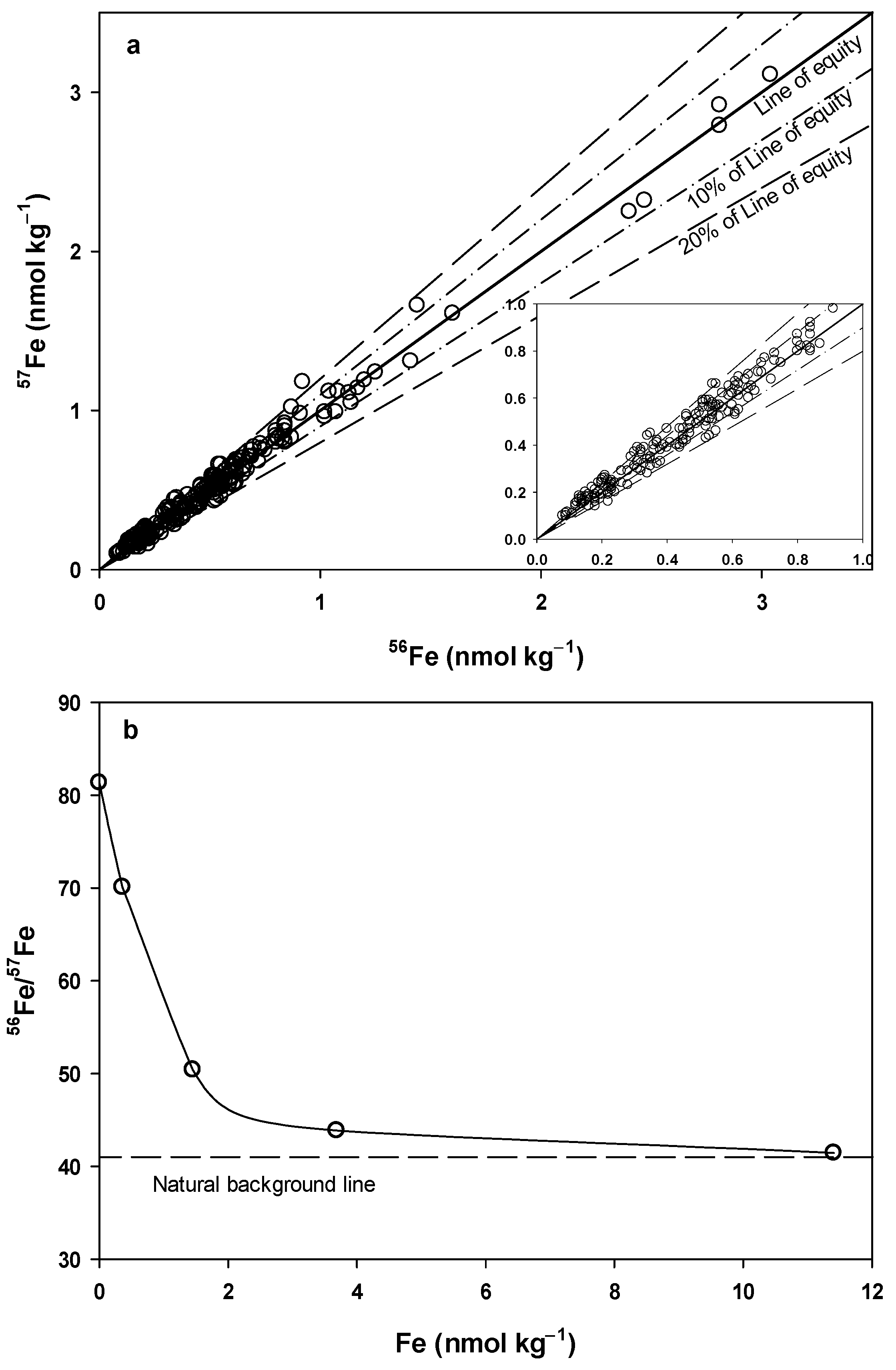
4.2.1. Recalculation of Fe

The high ratio of ⁵⁶Fe/⁵⁷Fe in the procedural blank, with respect to the natural isotopic abundance, suggests that the formation of ⁴⁰Ar¹⁶O⁺ increases the instrumental signal of ⁵⁶Fe. This is consistent with measured ⁵⁶Fe/⁵⁷Fe in seawater also being above natural isotopic abundance. Therefore, we validate Fe measurements by showing the blank subtracted Fe concentrations (with ⁵⁶Fe/⁵⁷Fe similar to the natural isotopic abundance) calculated based on ⁵⁶Fe and ⁵⁷Fe masses, which follow the line of equity with an agreement of better than 20% (Figure 2a). We further subtract the proportional contribution of ⁴⁰Ar¹⁶O⁺ and report the blank concentration of Fe (0.05 ± 0.02 nmol kg⁻¹, n = 77, Table 4). The contribution of ⁴⁰Ar¹⁶O⁺ is generally high for low Fe concentrations and noticeable up to 10 nmol kg⁻¹ (Figure 2b). Hence, blank subtraction is essential to measure Fe concentrations accurately in seawater.

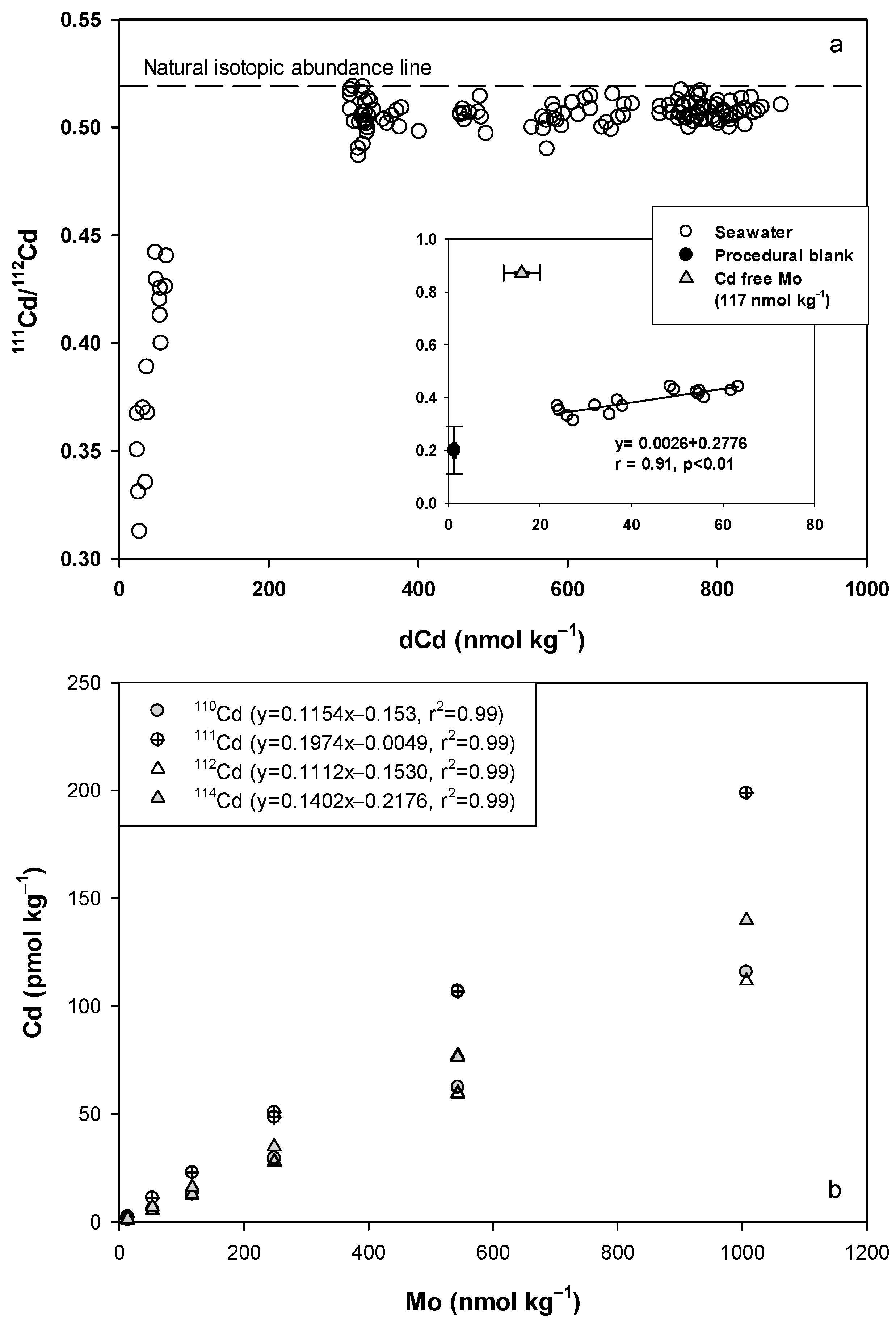
4.2.2. Recalculation of Cd

For Cd, the high ¹¹⁰Cd/¹¹¹Cd and low ¹¹⁰Cd/¹¹²Cd, ¹¹¹Cd/¹¹²Cd and ¹¹⁴Cd/¹¹²Cd of the blank as well as the low ¹¹¹Cd/¹¹²Cd of Cd-depleted seawaters (Figure 3a), relative to the respective natural isotopic abundances, indicates the preferential generation of ¹¹²Cd over ¹¹¹Cd from the plasma. This likely reflects the contribution of plasma derived ⁴⁰Ar¹⁶O⁺ on the instrumental signal of ¹¹²Cd. Cd-depleted seawater further results in a strong positive correlation between dCd and ¹¹¹Cd/¹¹²Cd, where the y-intercept characterizes the ¹¹¹Cd/¹¹²Cd-blank (Figure 3a), confirming a greater contribution of plasma-derived ¹¹²Cd. The presence of Mo in seawater also appeared to contribute to measured Cd despite the buffer pH (6.00 ± 0.2) chosen to limit Mo recovery [32]. Unlike the blanks, the observed instrumental masses for Cd-free Mo solutions showed that the preferential generation of ¹¹¹Cd and, to a lesser degree, ¹¹⁴Cd masses compared to others (Table 8). The measured Cd concentration (based on four Cd masses) of Cd-free solutions increased with increasing Mo concentrations and showed a strong positive correlation (Figure 3b). Given that the Mo concentration in seawater varies between 90–130 nmol kg⁻¹ (e.g., [33,34,35]), the equations of the Cd/Mo slopes were used to calculate the magnitude of added Cd resulting from polyatomic interference of Mo oxides. The added Cd ranged between 9.73–14.21 (based on ¹¹⁰Cd) and 10.23–14.85 pmol kg⁻¹ (based on ¹¹²Cd) with varying Mo in seawater. Based on ¹¹¹Cd and ¹¹⁴Cd signals, the added Cd was higher, between 17.76–25.66 pmol kg⁻¹ and 12.45–18.01 pmol kg⁻¹ respectively, because of their preferential generation over ¹¹⁰Cd and ¹¹²Cd. Therefore, we recommend monitoring ¹¹⁰Cd or ¹¹²Cd masses while measuring dCd for seawater. We additionally suggest using measured Mo concentration to calculate the magnitude of added Cd, and then to recalculate the actual Cd concentrations, particularly for low-dCd seawaters. We applied the above approach to recalculate the dCd concentration for the GEOTRACES GSP reference seawater (sampling location: 30° N, 140° W; consensus value: 2 ± 2 pmol L⁻¹). Using the Mo concentration of surface water of the North Pacific Ocean (107 ± 2.5 nM; [34]), dCd was recalculated with a range of 0.47–1.23 (0.99 ± 0.35) pmol kg⁻¹. This suggests that the proportional contribution of Mo-derived Cd constituted up to 90% of the measured Cd. However, for high-Cd seawater, the proportional contribution of Mo-derived Cd was less than 7%, and therefore had minimal effects on high-Cd concentrations.

4.3. Crossover Stations

For the crossover stations, the slight offset observed in the vertical profiles of Cu, Ni, and Co (Figure 1) potentially stem from differences in storage length times of the sample bottles. Offline preconcentrated samples were analysed approximately one year after sample collection and online preconcentrated samples approximately five years after collection. Previously, it has been suggested that even two years of sample storage at low pH may not be long enough to dissociate all organically complexed Cu [36]. Therefore, the offset between the vertical profiles of Cu may be due to the incomplete dissociation of organically complexed Cu in the offline preconcentrated samples. To our knowledge, the effect of sample storage time on Ni and Co concentrations has not been directly investigated. However, considering both metals are characterised by strong organic complexes [37,38], it is reasonable to suggest the offset in Ni and Co also stem from differences in sample storage time. For all other metals, the high degree of correlation between methods at the crossover stations and the intercalibration station corroborates method accuracy.

5. Conclusions

This study outlines the method development procedures for measuring dissolved metals from undiluted seawater performed over the past five years. In combination with the commercially available seaFAST (in both offline and online preconcentration setups), a single quadrupole ICP-MS yielded precise measurements for a suite of dissolved metals with a high degree of accuracy over a wide, oceanographically relevant concentration range. The plasma-generated ArO⁺ signal from the ICPMS instrument contributed 90% of the measured Fe in procedural blanks, while Mo-derived Cd constituted between 7% to 90% of the measured Cd in seawater. Among the various Cd isotopes derived from Cd-free seawater, the generation of ¹¹¹Cd (17.76–25.66 pmol kg⁻¹) was twice as high compared to the generation of ¹¹⁰Cd or ¹¹²Cd. As evidenced by the procedural blank concentrations, the data produced by the online setup posed less contamination risk. Procedural blanks for metals, and in particular Cd, can produce higher values in the offline setup due to unresolved Mo interferences, rather than due to the Cd contribution from the whole procedure itself. From these outcomes, we were able to recommend necessary measures using a simple instrumental set up to generate the highest-quality data for dissolved metals: (1) Monitor multiple isotopes of an analyte to track interferences within the mass spectrometer. (2) Blank subtraction is essential to measure Fe concentrations accurately in seawater. (3) Selecting ¹¹⁰Cd or ¹¹²Cd masses while analysing Cd from seawater. (4) For low-Cd seawater (<100 pmol kg⁻¹), first quantify the Mo concentration, then recalculate the Cd concentration based on the measured Mo concentration. Ultimately, this study shows that with careful post-processing, accurate analysis of trace metals over a wide range of seawater concentrations is achievable using a Q-ICP-MS, making it accessible to even financially constrained laboratories, and suitable for the demands of the GEOTRACES program.

References

1. Anderson, R.F.; Francois, R.H.G.M.; Frank, M.; Henderson, G.M.; Jeandel, C.; Sharma, M. GEOSECS to GEOTRACES: Lessons Learned from Large Programs Studying Ocean Chemistry. In AGU Fall Meeting Abstracts; American Geophysical Union: Washington, DC, USA, 2019; p. OS41A-05. [Google Scholar]
2. Bruland, K.W.; Franks, R.P. Sampling and analytical methods for the determination of copper, cadmium, zinc and nickel at the nanogram per litre level in seawater. Anal. Chim. Acta 1979, 28, 367–376. [Google Scholar] [CrossRef]
3. Wu, J.; Boyle, E.A. Low Blank Preconcentration Technique for the Determination of Lead, Copper, and Cadmium in Small-Volume Seawater Samples by Isotope Dilution ICPMS. Anal. Chem. 1997, 69, 2464–2470. [Google Scholar] [CrossRef] [PubMed]
4. Wells, M.L.; Bruland, K.W. An improved method for rapid preconcentration and determination of bioactive trace metals in seawater using solid phase extraction and high resolution inductively coupled plasma mass spectrometry. Mar. Chem. 1998, 63, 145–153. [Google Scholar] [CrossRef]
5. Bowie, A.R.; Achterberg, E.P.; Mantoura, R.F.C.; Worsfold, P.J. Determination of sub-nanomolar levels of iron in seawater using flow injection with chemiluminescence detection. Anal. Chim. Acta 1998, 361, 189–200. [Google Scholar] [CrossRef]
6. Colombo, C.; van den Berg, C.M.G. Simultaneous determination of several trace metals in seawater using cathodic stripping voltammetry with mixed ligands. Anal. Chim. Acta 1997, 337, 29–40. [Google Scholar] [CrossRef]
7. Kingston, H.M.; Barnes, I.L.; Brady, T.J.; Rains, T.C.; Champ, M.A. Separation of eight transition elements from alkali and alkaline earth elements in estuarine and seawater with chelating resin and their determination by graphite furnace atomic absorption spectrometry. Anal. Chem. 1978, 50, 2064–2070. [Google Scholar] [CrossRef]
8. King, D.W.; Lin, J.; Kester, D.R. Spectrophotometric determination of iron (II) in seawater at nanomolar concentrations. Anal. Chim. Acta 1991, 247, 125–132. [Google Scholar] [CrossRef]
9. Rapp, I.; Schlosser, C.; Rusiecka, D.; Gledhill, M.; Achterberg, E.P. Automated preconcentration of Fe, Zn, Cu, Ni, Cd, Pb, Co, and Mn in seawater with analysis using high-resolution sector field inductively-coupled plasma mass spectrometry. Anal. Chim. Acta 2017, 976, 1–13. [Google Scholar] [CrossRef] [Green Version]
10. Jackson, S.L.; Spence, J.; Janssen, D.J.; Ross, A.R.S.; Cullen, J.T. Determination of Mn, Fe, Ni, Cu, Zn, Cd and Pb in seawater using offline extraction and triple quadrupole ICP-MS/MS. J. Anal. At. Spectrom. 2018, 33, 304–313. [Google Scholar] [CrossRef]
11. Wuttig, K.; Townsend, A.T.; van der Merwe, P.; Gault-Ringold, M.; Holmes, T.; Schallenberg, C.; Latour, P.; Tonnard, M.; Rijkenberg, M.J.A.; Lannuzel, D.; et al. Critical evaluation of a SeaFAST system for the analysis of trace metals in a wide range of marine samples. Talanta 2019, in press. [Google Scholar] [CrossRef]
12. Strivens, J.E.; Brandenberger, J.M.; Johnston, R.K. Data trend shifts induced by method of concentration for trace metals in seawater: Automated online preconcentration vs. borohydride reductive coprecipitation of nearshore seawater samples for analysis of Ni, Cu, Zn, Cd, and Pb via ICP-MS. Limnol. Oceanogr. Methods 2019, 17, 266–276. [Google Scholar] [CrossRef]
13. Vassileva, E.; Wysocka, I.; Orani, A.M.; Quétel, C. Off-line preconcentration and inductively coupled plasma sector field mass spectrometry simultaneous determination of Cd, Co, Cu, Mn, Ni, Pb and Zn mass fractions in seawater: Procedure validation. Spectrochim. Acta Part B At. Spectrosc. 2019, 153, 19–27. [Google Scholar] [CrossRef]
14. Wysocka, I.; Vassileva, E. Method validation for high resolution sector field inductively coupled plasma mass spectrometry determination of the emerging contaminants in the open ocean: Rare earth elements as a case study. Spectrochim. Acta Part B At. Spectrosc. 2017, 128, 1–10. [Google Scholar] [CrossRef]
15. Behrens, M.K.; Muratli, J.; Pradoux, C.; Wu, Y.; Böning, P.; Brumsack, H.J.; Goldstein, S.L.; Haley, B.; Jeandel, C.; Paffrath, R.; et al. Rapid and precise analysis of rare earth elements in small volumes of seawater—Method and intercomparison. Mar. Chem. 2016, 186, 110–120. [Google Scholar] [CrossRef] [Green Version]
16. Vassileva, E.; Wysocka, I. Development of procedure for measurement of Pb isotope ratios in seawater by application of seaFAST sample pre-treatment system and SF ICP-MS. Spectrochim. Acta Part B At. Spectrosc. 2016, 126, 93–100. [Google Scholar] [CrossRef]
17. Poehle, S.; Schmidt, K.; Koschinsky, A. Determination of Ti, Zr, Nb, V, W and Mo in seawater by a new online-preconcentration method and subsequent ICP-MS analysis. Deep. Res. Part I Oceanogr. Res. Pap. 2015, 98, 83–93. [Google Scholar] [CrossRef]
18. Tanner, S.D.; Baranov, V.I. Theory, Design, and Operation of a Dynamic Reaction Cell for ICP-MS. At. Spectrosc. 1999, 20, 45–78. [Google Scholar] [CrossRef]
19. Cloete, R.; Loock, J.C.; Mtshali, T.; Fietz, S.; Roychoudhury, A.N. Winter and summer distributions of Copper, Zinc and Nickel along the International GEOTRACES Section GIPY05: Insights into deep winter mixing. Chem. Geol. 2019, 511, 342–357. [Google Scholar] [CrossRef]
20. Cloete, R.; Loock, J.C.; van Horsten, N.R.; Fietz, S.; Mtshali, T.N.; Planquette, H.; Roychoudhury, A.N. Winter biogeochemical cycling of dissolved and particulate cadmium in the Indian sector of the Southern Ocean (GEOTRACES GIpr07 transect). Front. Mar. Sci. 2021, 8, 1014. [Google Scholar] [CrossRef]
21. Cloete, R.; Loock, J.C.; van Horsten, N.R.; Menzel Barraqueta, J.-L.; Fietz, S.; Mtshali, T.N.; Planquette, H.; García-Ibáñez, M.I.; Roychoudhury, A.N. Winter dissolved and particulate zinc in the Indian Sector of the Southern Ocean: Distribution and relation to major nutrients (GEOTRACES GIpr07 transect). Mar. Chem. 2021, 236, 104031. [Google Scholar] [CrossRef]
22. Cutter, G.; Casciotti, K.; Croot, P.; Geibert, W.; Heimbürger, L.-E.; Lohan, M.; Planquette, H.; van de Flierdt, T. Sampling and Sample-Handling Protocols for GEOTRACES Cruises; GEOTRACES International Project Office: Toulouse, France, 2017. [Google Scholar]
23. Byrd, J.T.; Andreae, M.O. Dissolved and particulate tin in North Atlantic seawater. Mar. Chem. 1986, 19, 193–200. [Google Scholar] [CrossRef]
24. McKelvey, B.A.; Orians, K.J. Dissolved zirconium in the North Pacific Ocean. Geochim. Cosmochim. Acta 1993, 57, 3801–3805. [Google Scholar] [CrossRef]
25. Bekov, G.I.; Letokhov, V.S.; Radaev, V.N.; Baturin, G.N.; Egorov, A.S.; Kursky, A.N.; Narseyev, V.A. Ruthenium in the ocean. Nature 1984, 312, 748–750. [Google Scholar] [CrossRef]
26. Liu, K.; Gao, X.; Li, L.; Chen, C.T.A.; Xing, Q. Determination of ultra-trace Pt, Pd and Rh in seawater using an off-line pre-concentration method and inductively coupled plasma mass spectrometry. Chemosphere 2018, 212, 429–437. [Google Scholar] [CrossRef]
27. Feldmann, I.; Jakubowski, N.; Stuewer, D. Application of a hexapole collision and reaction cell in ICP-MS Part I: Instrumental aspects and operational optimization. Fresenius J. Anal. Chem. 1999, 365, 415–421. [Google Scholar] [CrossRef]
28. Yamada, N. Kinetic energy discrimination in collision/reaction cell ICP-MS: Theoretical review of principles and limitations. Spectrochim. Acta Part B At. Spectrosc. 2015, 110, 31–44. [Google Scholar] [CrossRef]
29. Smedley, P.L.; Kinniburgh, D.G. Molybdenum in natural waters: A review of occurrence, distributions and controls. Appl. Geochem. 2017, 84, 387–432. [Google Scholar] [CrossRef] [Green Version]
30. Arnold, T.; Harvey, J.N.; Weiss, D.J. An experimental and theoretical investigation into the use of H2 for the simultaneous removal of ArO+ and ArOH+ isobaric interferences during Fe isotope ratio analysis with collision cell based Multi-Collector Inductively Coupled Plasma Mass Spectrometry. Spectrochim. Acta Part B 2008, 63, 666–672. [Google Scholar] [CrossRef]
31. Sadagopa Ramanujam, V.M.; Yokoi, K.; Egger, N.G.; Dayal, H.H.; Alcock, N.W.; Sandstead, H.H. Polyatomics in zinc isotope ratio analysis of plasma samples by inductively coupled plasma-mass spectrometry and applicability of nonextracted samples for zinc kinetics. Biol. Trace Elem. Res. 1999, 68, 143–158. [Google Scholar] [CrossRef]
32. Biller, D.V.; Bruland, K.W. Analysis of Mn, Fe, Co, Ni, Cu, Zn, Cd, and Pb in seawater using the Nobias-chelate PA1 resin and magnetic sector inductively coupled plasma mass spectrometry (ICP-MS). Mar. Chem. 2012, 130–131, 12–20. [Google Scholar] [CrossRef]
33. Schlitzer, R.; Anderson, R.F.; Dodas, E.M.; Lohan, M.; Geibert, W.; Tagliabue, A.; Bowie, A.; Jeandel, C.; Maldonado, M.T.; Landing, W.M.; et al. The GEOTRACES Intermediate Data Product 2017. Chem. Geol. 2018, 493, 210–223. [Google Scholar] [CrossRef]
34. Collier, R.W. Molybdenum in the Northeast Pacific Ocean. Limnol. Oceanogr. 1985, 30, 1351–1354. [Google Scholar] [CrossRef]
35. Ho, P.; Lee, J.-M.; Heller, M.I.; Lam, P.J.; Shiller, A.M. The distribution of dissolved and particulate Mo and V along the U.S. GEOTRACES East Pacific Zonal Transect (GP16): The roles of oxides and biogenic particles in their distributions in the oxygen deficient zone and the hydrothermal plume. Mar. Chem. 2018, 201, 242–255. [Google Scholar] [CrossRef]
36. Posacka, A.M.; Semeniuk, D.M.; Whitby, H.; Van Den Berg, C.M.; Cullen, J.T.; Orians, K.; Maldonado, M.T. Dissolved copper (dCu) biogeochemical cycling in the subarctic Northeast Pacific and a call for improving methodologies. Mar. Chem. 2017, 196, 47–61. [Google Scholar] [CrossRef]
37. Saito, M.A.; Moffett, W. Cobalt and nickel in the Peru upwelling region: A major flux of labile cobalt utilized as a micronutrient. Glob. Biogeochem. Cycles 2004, 18, GB4030. [Google Scholar] [CrossRef] [Green Version]
38. Morel, F.M.M.; Milligan, A.J.; Saito, M.A. Marine Bioinorganic Chemistry: The Role of Trace Metals in the Oceanic Cycles of Major Nutrients. In Treatise on Geochemistry, 2nd ed.; Holland, H.D., Turekian, K.K., Eds.; Elsevier: Amsterdam, The Netherlands, 2014; pp. 123–150. [Google Scholar] [CrossRef]
Figure 1. Offline vs. Online vertical profiles of trace metals. For some data points, error bars are smaller than symbol size and not visible. The data point isolated within a circle for Cu represents potential contamination during sample handling.
Minerals 11 01289 g001
Figure 2. (a) Measured Fe concentrations, calculated based on 57Fe and 56Fe masses, follow the line of equity. (b) measured 56Fe/57Fe ratios are presented for a range of Fe concentration.
Minerals 11 01289 g002
Figure 3. (a) Measured 111Cd/112Cd ratios for a wide range of seawater Cd concentration. (b) MoO+-derived Cd concentrations are shown with a range of mono-element Mo solutions.
Minerals 11 01289 g003