Possible Pitfalls in the Analysis of Minerals and Loose Materials by Portable XRF, and How to Overcome Them

Abstract

Portable X-ray fluorescence spectroscopy is now widely used in almost any field of geoscience. Handheld XRF analysers are easy to use, and results are available in almost real time anywhere. However, the results do not always match laboratory analyses, and this may deter users. Rather than analytical issues, the bias often results from sample preparation differences. Instrument setup and analysis conditions need to be fully understood to avoid reporting erroneous results. The technique’s limitations must be kept in mind. We describe a number of issues and potential pitfalls observed from our experience and described in the literature. This includes the analytical mode and parameters; protective films; sample geometry and density, especially for light elements; analytical interferences between elements; physical effects of the matrix and sample condition, and more. Nevertheless, portable X-ray fluorescence spectroscopy (pXRF) results gathered with sufficient care by experienced users are both precise and reliable, if not fully accurate, and they can constitute robust data sets. Rather than being a substitute for laboratory analyses, pXRF measurements are a valuable complement to those. pXRF improves the quality and relevance of laboratory data sets.

1. Introduction

Portable or handheld X-ray fluorescence spectroscopy (pXRF) has been a widely used on-site analytical tool since 1995 in many geoscientific fields—i.e., [1,2,3,4,5,6,7]. These include mineral exploration, environmental investigations and remediation, process monitoring, and industrial minerals.

The reliability and accuracy of this technique has been extensively discussed and compared with laboratory analyses on the same samples [8,9,10,11,12,13]. In many cases, this discussion suffered major flaws, which led to misinterpretations of discrepancies between pXRF and laboratory results. Among these, let us mention the comparison with ICP analyses on digested samples; the comparison of field measurements on roughly prepared samples with lab quality pulps, not taking into account grain size or moisture effects; and the comparison of repeated field measurements with one laboratory sample with undocumented representativity.

It must be reminded here that pXRF analyses can be performed in two markedly different situations:

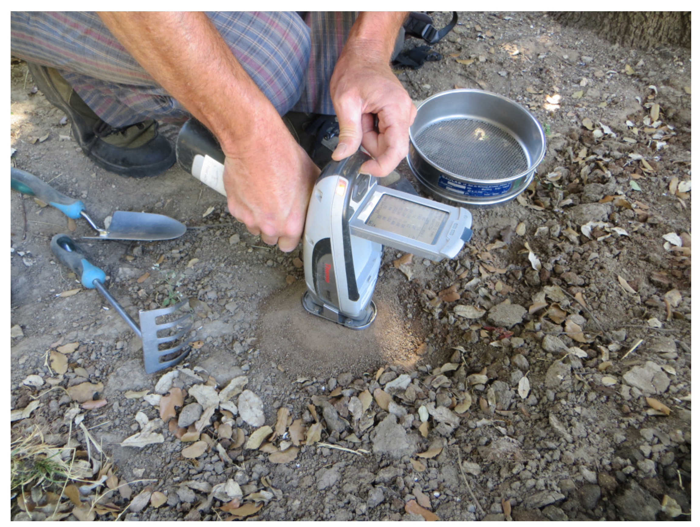
• On-site, with a simplified sample preparation or no preparation, the results being used for sample screening or for orientating further site investigations,
• On-site or off-site, with the best available sample preparation, and using QA/QC procedures similar to a laboratory.

The former cannot reach laboratory level accuracy, while the latter allow satisfactory relationships with laboratory results, provided that attention is paid to the specificities of pXRF analysis. This is the purpose of the present paper.

Both strategies are valid and useful for geoscientific investigations, but their results must not be mixed.

This paper reviews some of the most important—and often overlooked—issues to be taken into account while using pXRF for the analysis of minerals and geomaterials. Other applications of pXRF include process control in the mining, metal and recycling industries, agricultural soil analysis, compliance testing and non-destructive analysis of art or archaeological items.

2. Materials and Methods

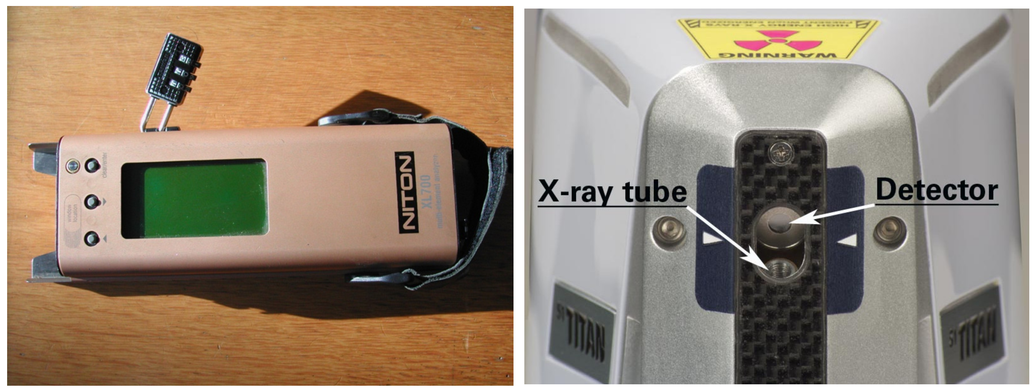
2.1. pXRF Instruments

The experience acquired by the authors, mainly with BRGM, dates back to 2000 and the earlier pXRF spectrometers, based on isotopic sources [14]. A Niton XL703S/XL723 was first used (Figure 1 left).

Portable X-ray fluorescence spectrometers are now based on a similar scheme. A battery-powered X-ray tube and a detector (Silicon Drift SDD detectors replacing traditional Si-PIN detectors, [4]) are in optical connection with the sample through a thin window at the front of the instrument (Figure 1 right).

From 2005 onwards, the authors used several Niton XLt tube-type spectrometers (XLt792, XLt999, [14,15,16]) which are still in operation. These instruments were dedicated mainly to the analysis of contaminated soil and were able to analyse medium or heavy elements comprised between K and Pb.

Spectrometers with improved detection capabilities (Niton XL3t980, Olympus Delta Premium, and occasionally Bruker Titan, Oxford XMET, Olympus Vanta) were used since 2010 whenever the analysis of lighter elements (Al, Si, P, S, Cl) was desirable alongside heavier elements, or for improved analytical performance [17,18] and numerous BRGM reports.

2.2. pXRF Operating Conditions and Methods

In addition to soil, many geological or geo-derived matrices were analysed (sediments, rocks, mining, and industrial waste). Generally, the Compton-based soil calibration mode was used for most samples, while the fundamental parameters mining mode was used whenever the elements of concern (Pb, Zn, Cu, As, Cr, etc.) were found to be abundant (>0.5% to 1%). Further details on these modes can be found in [4,10,19].

Most analyses were obtained on-site, either directly from roughly prepared samples, or after some homogenisation (Figure 2). Some analyses were performed on a measurement bench at the camp or in the laboratory, allowing a longer counting time if necessary.

Operating parameters evolved along the years, with an increased number of filters and shorter counting times. Filters are used by instrument manufacturers to improve accuracy while taking into consideration spectral conditions for each group of elements (light, medium, or heavy) and excitation parameters. Earlier analyses on two filters needed a total 120 s on-site (2 × 60 s) and up to 5 min on the bench [15]. Current total counting times range from 30 to 90 s, depending on the number of filters and the targeted elements. Most analyses were performed using the factory calibration, with no correction factor. Such factors can be useful when all samples have a similar matrix, allowing on-site decisions at mine or waste management sites [18]. When variable matrices are expected (most geochemical surveys), it is safer to record raw analyses and post-process them once the survey is completed, to get more accurate results.

A large part of the observations discussed below were obtained in the laboratory, with off-standard conditions. All samples are dried and ground to 100 µm, prepared in triplicate in a filmless tube or cup; when a film is used, the type of film on the cup depends on the purpose; multiplying samples and cups was preferred to multiplying measurements on a single cup (Figure 8). These experimental conditions were selected on the basis of the observations collected during routine field surveys. One of the benefits of pXRF instruments is to give the opportunity to modify operating parameters to test hypotheses, on the field and later in the laboratory, when unexpected results are obtained. An example of this is observing abnormally high concentrations of an element which should not be abundant in this context. This may warn the operator of possible element interference (discussed in Section 3.4).

2.3. Laboratory Analysis Methods

The laboratory results described here were obtained using a large range of instruments, according to the needs of the projects from which the examples described in this paper are extracted. Most pXRF surveys performed by the authors comprised a laboratory control for accuracy.

In most cases, laboratory controls were done by ICP-AES (Inductively coupled plasma atomic emission spectroscopy) using aqua regia, three or four acid digestion, or alkali sintering when refractory minerals were expected. Controls using a laboratory XRF would be more relevant, but this option was not often available. For trace elements at very low concentrations (<5 mg/kg), ICP-MS (Inductively coupled plasma mass spectrometry) was most often used.

3. Results

3.1. Analytical Modes in pXRF—Relevance and Applicability to Geochemical Investigations

3.1.1. The Different Analytical Modes

Most X-ray fluorescence analysers have one or more analytical modes (

Table 1. Mode names, according to analytical mode and manufacturer.

Method	Fundamental Parameters (FP)	Compton	Empirical	Positive Material Identification (PMI)
Names	Mining, Geochemistry, Alloys, Precious metals, Plastics	Soil		Consumer Safety, RoHS, WEEE, Fast Identification
Materials analysed	Rocks, ores, soils, waste, plastics, and alloys	Rocks, soils, and sediments data	All matrices, paint, fine deposit, dust	Minerals, waste, alloys

RoHS: Restriction of Hazardous Substances control for consumer goods. WEEE: Waste Electrical and Electronic Equipment control.

). Their name varies from one manufacturer to another depending on the material to be analysed (soil, mining/Geochem, alloy, plastic, etc.) or the calibration method (fundamental parameters (FP)), Compton normalisation, empirical method, and PMI (Positive Material Identification, comparison of spectra using a spectra library).

3.1.2. Compton Normalisation

Compton normalisation provides the best results for a wide range of environmental tests and for certain mining applications, in particular when it is necessary to measure contents below 1% in samples composed mainly of light elements. It works best when total dilution of the element in the sample can be assumed, similarly to analytical methods aimed at trace elements. This explains why, besides its usual name (Soil), it is applicable to almost any homogeneous solid sample.

Principle

The sample matrix affects radiation scattering. Compton scattering is proportional to the light elements’ contents in the sample and directly depends on the intensity of the Compton peak. Compton normalisation calibration consists of analysing a single, well-characterised standard in order to record the intensity of the Compton peak. While performing an analysis with a XL3t980 equipped with an Ag anode, the Compton peaks in the sample spectra are normalised to a “standard” Compton peak (Figure 3). This method reduces the problems associated with matrix effects, which vary from sample to sample. Compton normalisation is similar to the use of internal standards for analysis.

Limitations of the Method

• The device software subtracts a background noise signal equivalent to a matrix containing 99% SiO₂ (also roughly equivalent to 99% carbonates). The matrix density is therefore assumed to be of the order of 1.8 g·cm⁻³. If this mode is used for different matrices, the background noise is poorly taken into account, and lower or negative values can be obtained (i.e., real background noise above the subtracted noise, and negative background residue), or overestimated (i.e., actual background noise below the subtracted noise, a positive residue being added to the potentially present peak).
• The extraction is done only on the peak height (centre strip) and not on the shape (which would be more precise with a deconvolution of line profile). Moreover, the ratio between the lines of the same pure element is unfortunately known to be not constant, depending on matrix density.
• The extracted peak intensities are converted into concentrations by:

  (a)

  the relationship between the intensity of the element peak with the intensity of the Compton peak of the tube, or a region of interest assumed to bear no peak (depending on the filter used, because the low filter cannot measure the Compton peak).

  (b)

  a calibration of this ratio with soil standards entered in the device.

  (c)

  no additional correction (unlike fundamental parameters).

3.1.3. Fundamental Parameters (FP)

The fundamental parameters are used to measure samples of unknown chemical composition in which the concentrations of light and heavy elements can vary from mg/kg to a high percentage. FP analysis is used to simultaneously compensate for a wide variety of geometric effects (including small fragments of various shapes), plus X-ray absorption and secondary and tertiary fluorescence effects. FP is the preferred tool when major and trace elements have to be analysed simultaneously, especially for mining applications, precious metals, and metal alloys. It is also adequate when dealing with unknown samples, for which the range for the elements of concern may vary between trace and major level (i.e., ores, wastes), and for samples for which geometric particles heterogeneity or particle absorption may affect XRF measurements.

Principle

The fundamental parameters are calibrated without any standard. Calibration is based on the known physics of the spectrometer’s response to pure elements. Mathematical algorithms for the device are used to correct matrix effects.

Matrix correction methods by FPs make possible a “universal” factory calibration of the instrument. The term universal means that calibration is independent of the type of sample provided that the physical assumptions made during the development of the calibration are respected. In the general case, these assumptions are:

• sample homogeneity;
• completeness, which implies that all the elements are measured or estimated by stoichiometry or by complement to 100%.

The calibration must then be transferred to the final device, to take into account the differences with the reference device. For this purpose, a set of stable samples (generally glasses) are measured on the reference device and on the final device; the ratio of the intensities measured on the two devices is then applied to the calibration coefficients.

Limitations of the Method

The FP mode is not “pure” FP calibration. Niton also uses for its Mining mode the Compton peaks, which provide information on the entire matrix, to calculate the balance (difference between total and 100%).

The physics of X-rays for FP mode assumes that all atoms are intimately mixed at the atomic level. This is not the case in mixtures of particles and mineral assemblages, in which grain sizes can be 10 µm, 100 µm, 1 mm, and more. The fluorescence X-rays intensity varies significantly depending on the particle size distribution. This phenomenon cannot be avoided regardless of the care taken in milling.

It is extremely difficult, if not impossible, to obtain standards having the same particle size distribution as the sample to be analysed. For standard preparation, the milling time must be sufficient to obtain a sample of which at least 95% of the mass passes through a 200-mesh sieve, i.e., 74 μm. The standards used by the manufacturers are generally provided by the National Institute of Standards and Technology (NIST), but all laboratory standards (CRMs, Certified Reference Materials) of the same type and preparation can be used.

3.1.4. Empirical Method

The empirical method (called User mode on Niton and Olympus), is based on a preliminary analysis of known samples to obtain the counting intensity, which is then plotted using software (Excel) to generate the calibration curve. This curve data is then fed back into the analyser, which uses it to get immediate results. The empirical test modes are only suitable for the measurement of samples for which the chemical compositions are within the narrow calibration range for a given matrix; and interference (spectral and matrix) must be taken into account during calibration.

Principle

Most pXRFs allow their user to create their own calibration curves. The empirical calibration method is based on a series of standards for calculating the calibration parameters. The instrumental response to CRM standard samples is measured and used to create calibration curves from them. Standards should contain all elements of interest and those that may interfere.

This method is effective if the matrix composition of the CRM standard samples used is close to the matrix of the samples to be analysed. This condition is rarely achieved, and in many cases, it is better to prepare SRMs (standard reference materials) from a matching matrix material (for instance, a barren sample from a mine’s host rocks), by spiking it with known amounts of the elements of interest. Achieving absolute accuracy may be time consuming if variable matrixes are present, but the method remains highly sensitive and reveals small variations for each measured element.

Limitations of the Method

Empirical calibration can be used for all types of samples, provided that you have enough CRM standards, or if you prepare your own from well-known materials. It is essential to have standards with higher concentrations in all elements of concern, as empirical calibration is only applicable by interpolation. Any attempt to extend it by extrapolation is likely to result in high bias in the upper range of concentrations.

3.1.5. Matching Library Method (PMI)

Comparison of spectra (PMI, Positive Material Identification) is mainly used for the identification of alloys, for sorting metallic waste to be recycled, and for the detection of undesirable substances in consumer products or in waste for recycling.

Principle

In the spectrum comparison mode, pXRF compares the spectrum of an observed sample with those stored in its memory. The most similar is displayed, along with a figure quantifying the correlation between the two spectra. This method makes it possible to quickly compare (in three seconds) a sample with the spectra of known alloys stored in the pXRF.

pXRF devices have usually factory-installed spectra libraries. Depending on their needs, operators can also create their library by testing alloys or other known substances and gathering their spectra. Spectral comparison produces precise chemical information if the reference spectra have been obtained on assayed samples.

Limitations of the Method

A large library is required to be able to correctly identify unknown samples. For mining, the library has to be built using laboratory and pXRF analyses of all the rock matrices that can be encountered during routine analyses. Another limitation is bound to the matrix effects that play a key role in the quantitative determination of each targeted elements.

3.2. Impact of the Composition of Windows and Other Film Products Used for Protection in pXRF, and Sample Bag Applications

Several types of membranes and films can be used to protect the device and prepare samples in cups or in bags with different compositions. Depending on the objective of the analyses (nature of the elements and the preparation of the samples, accuracy of the measurements, etc.), it is important to choose the different membranes in order to make correct analyses but also to protect the device.

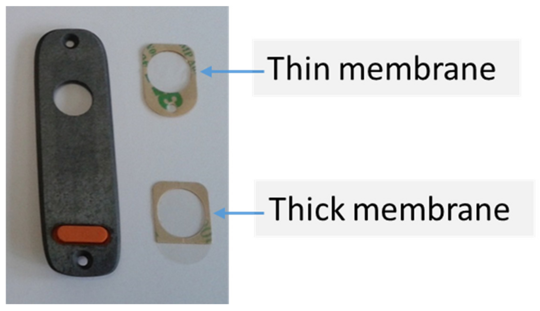
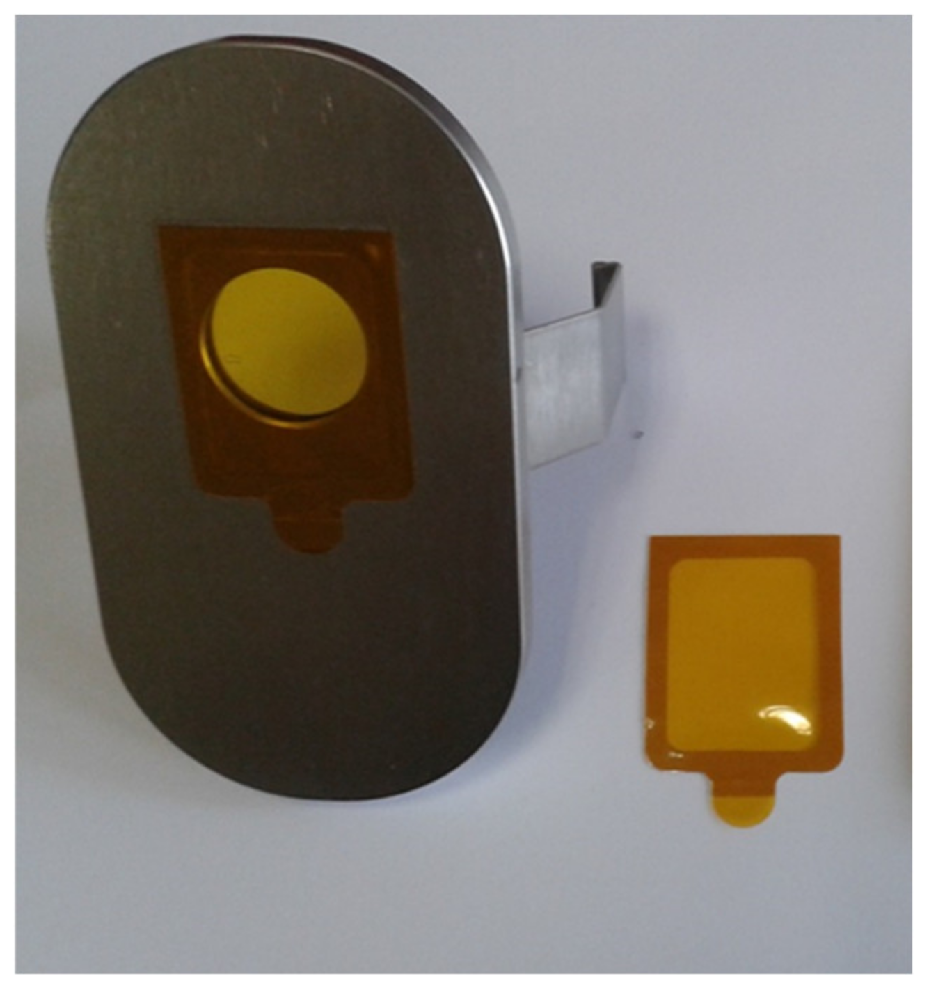
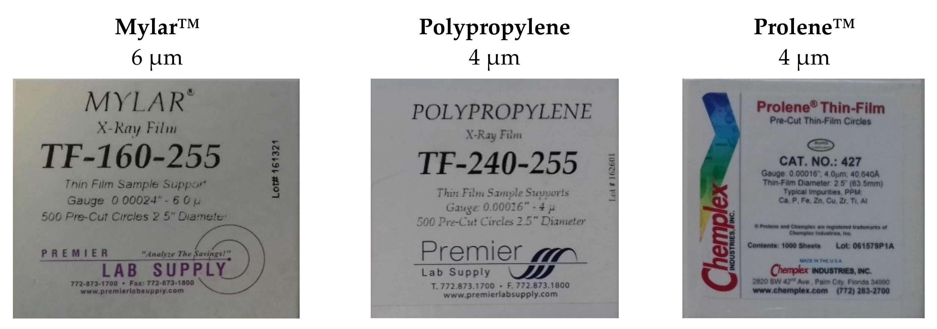
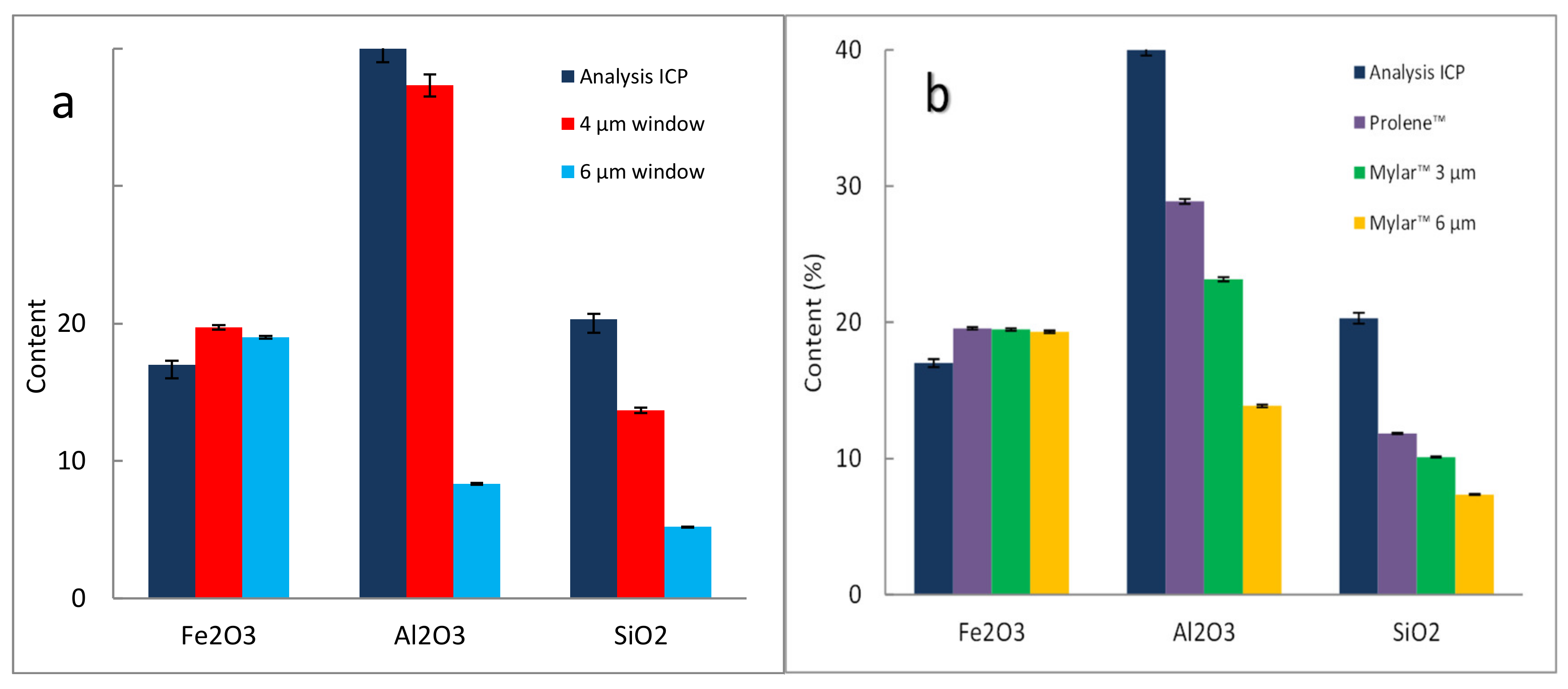
3.2.1. Spectrometer Window

This section aims at comparing window settings applicable to field analysis of solids. Other settings (beryllium window, windows for liquids analysis, etc) are not addressed. The window on the nose of the device (Figure 4) is built of polymer film:

• Thick membranes (6 to 7 µm in polypropylene, Mylar™ or Kapton™) for analysing mainly heavy elements (e.g., Pb, Zn, and Cu). For Niton spectrometers (Xlt, Xl2t, Xl3t, and Xl5), Olympus (Delta), Vanta: Mylar, or Kapton, Bruker (Kapton), Hitachi (mylar), SciAps (Kapton);
• Thin membranes (4 µm) allowing the analysis of light elements (Niton Xl3t and Xl5: Prolene™), Olympus (Delta and Vanta: Prolene™), Bruker (Ultralene^TM), Hitachi (polypropylene), SciAps (Prolene™).

This issue was less critical on earlier instruments which did not attempt to analyse light elements [10,20]. Even so, absorption issues were observed and quantified by these authors. The use of the particularly ineffective LDPE (Low-density polyethylene) for windows [19] was discontinued since then. In another study [20], the authors compared various spectrometer windows settings (air, vacuum, and helium) and various window screens (Prolene™, Kapton™, and Mylar™) in various thicknesses (3 to 7 µm). They observed that thin Prolene™ (<4 µm) achieved better photon energy (up to +100% in transmission effectiveness).

Numerous studies showed the effect of the film composition on element quantification [7,12,20,21,22]. Film impurities were measured by [23,24] who identified higher contamination (P, Ca, Cu, and Zn) of Kapton™ and Mylar™, while Prolene™ showed only minor light element contamination (Al and Si). It is therefore important to keep a full track record of the of the measurement conditions, as most users have their own habits or procedures.

3.2.2. Spectrometer Protection Shield

Spectrometer nose shields are proposed by a few manufacturers (Figure 5) to cope with rough field conditions and protect the nose window. This thick Kapton™ membrane does not allow the analysis of light elements.

For instruments without any protection shield, Prolene™ or Mylar™ films, available as rolls, can be placed on the head of the spectrometer and constitute a protection against stains, dust, or moisture. They are certainly less resistant than the Kapton™ mask, but much less absorbent. This layout is well suited to the Olympus Delta and Vanta, Bruker Titan and Tracer, and SciAps X series.

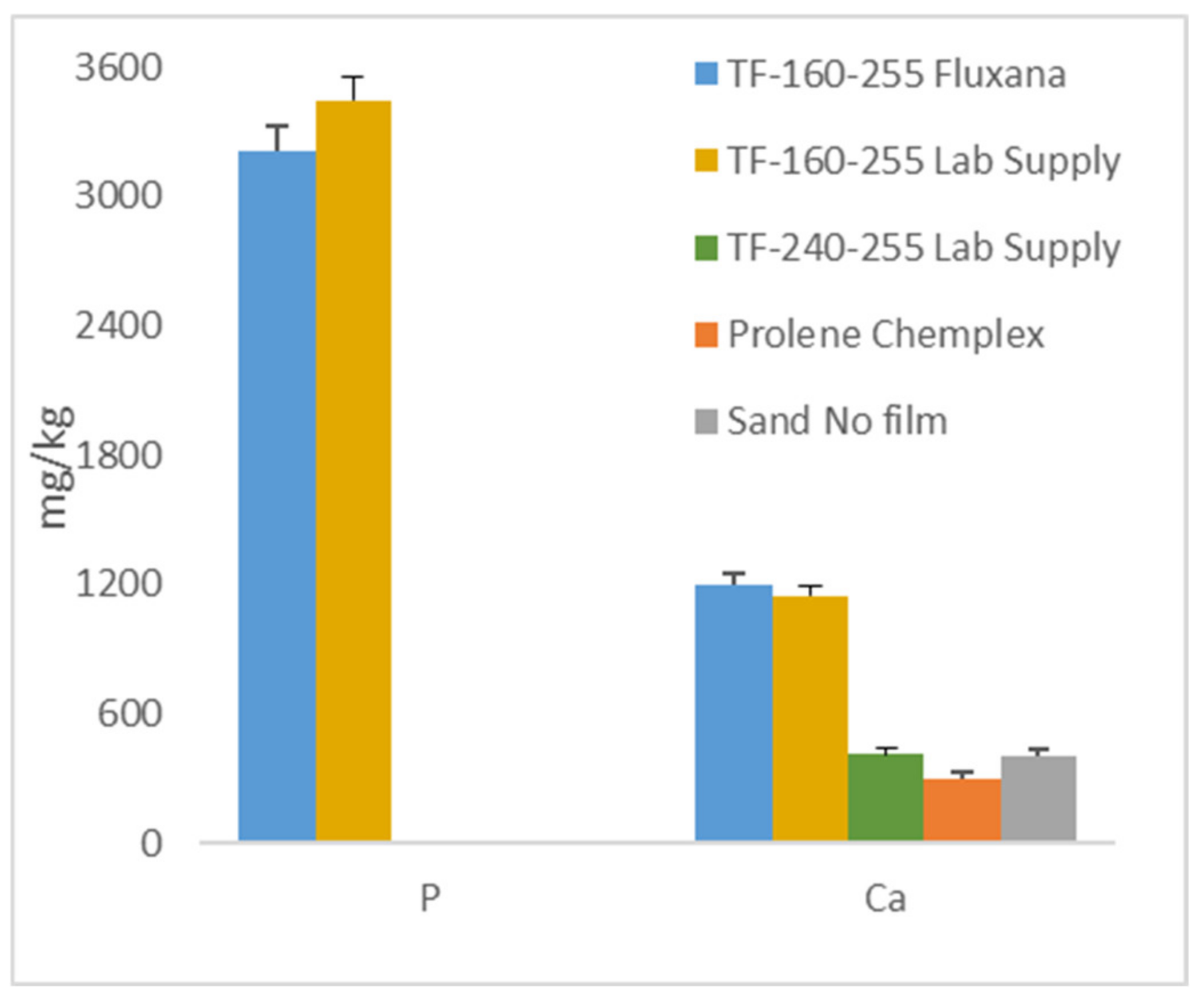
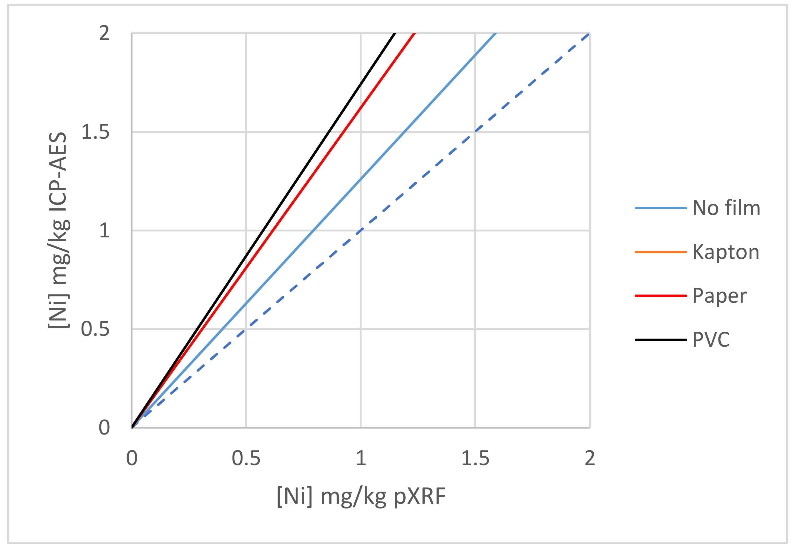
3.2.3. Films Used for the Cups

Depending on the supplier, the name, thickness, and composition of cup films varies (Figure 6):

The most common types of films are addressed below.

Mylar™ is used because of its strength, even if very thin (down to 1.5 µm), and low cost. Its transmission characteristics are poorer than most other films. The 6 µm film can be used only for analysing high Z elements, while the 3.6 µm film may be used for elements down to K and Ca. The 1.5 µm film was used for lighter elements, but is difficult to handle, and is not widely used for routine analysis. Mylar™ is more resistant than Prolene™ due to additives containing Al, Si, P, and Ca, and trace amounts of S, K, Mn, Sb, Fe, Zn, Cu, and Ti.

Polypropylene is now the most popular film for windows. It is inexpensive and is chemically resistant. Its transmission is higher than Mylar^TM’s. As 6.3 µm thick film, it can be used for analysing elements from K up in the periodic table. Thinner films are preferable for elements from Al to S. Polypropylene has poor tensile strength and stretches easily, hence poorer reproducibility than Mylar, and may soften or wrinkle if exposed to hydrocarbons.

Prolene™, Ultralene™, and Spectrolene™ films are chemically similar to polypropylene, and offer similar resistance properties in 6 µm and 4 µm thicknesses. Their X-ray transmissions are the best available, so they are the best choice when analysing low atomic number elements (Mg to S). Prolene™ contains far less impurities than Mylar™ and Kapton™. The 4 µm film is still easy to handle and resistant in mild use conditions. The only issue is the higher cost of these films.

3.2.4. Sample Bags and Other Films Used for Packaging

The practice of analysing routine samples through sample bags is frequent in the mining industry and exploration, despite the signal absorption it implies. It assumes that, if a single sample bag type is used throughout a project, the resulting bias will be the same for all samples, and will not affect sample ranking, maps, logs, or dynamic sampling strategy.

Taking measurements at different places on a sample bag was proposed by [25] as a way to control sample homogeneity. Reference [26] mentioned that this practice did not prevent public reporting of data under the JORC Code, as long as it is duly mentioned. Reference [27] investigated several types of plastic bags commonly used, but not cloth (calico) bags, with signal attenuation from −20 to −90% depending on bag type. Reference [28] compared the attenuation by LDPE bags, a proprietary type of bag and Prolene^TM film on cups. They concluded a minor effect on Zn (representing heavier elements), an observable but acceptable effect on K and Ca, and a major effect on Si. These conclusions were confirmed by our own observations during routine work.

Reference [10] showed that attenuation was not the only issue, as the plastic material could contain some metals too (such as polymerisation catalysts). This suggests that LDPE is more suitable than HDPE (High-density polyethylene), due to a lower amount of additives. Reference [29] tested a variable number of layers of polyethylene film against adsorption and reported a linear correlation with the number of layers. Reference [30] reported 5–10% attenuation in plastic bags, but more interestingly reported both positive and negative bias according to the element. Reference [20] reported that even 50 µm thick LDPE bags affected both attenuation and RSD of measurements. The effect of plastic bags cannot be reduced to a linear attenuation and must be cross-checked with laboratory analyses.

A particular case of sample covering by film is routine analysis of drill-hole cores, which requires efficiency and easy handling. It was investigated first for core scanners and quantitative geochemical logging [31] but the use of pXRF for the same purpose became widespread. This is also based on the reproducibility and sensitivity to small geochemical variations of pXRF measurements, regardless of their absolute accuracy. An extra difficulty results from thickness variations in the water film that is trapped between the protective foil and the core surface. Unless Al and Si measurements are the key objective, a thicker polypropylene or Mylar™ film will be used to cover the core. As for windows or cup films, the key issues are (1) always using the same material, and (2) keeping a full track record along with measurements.

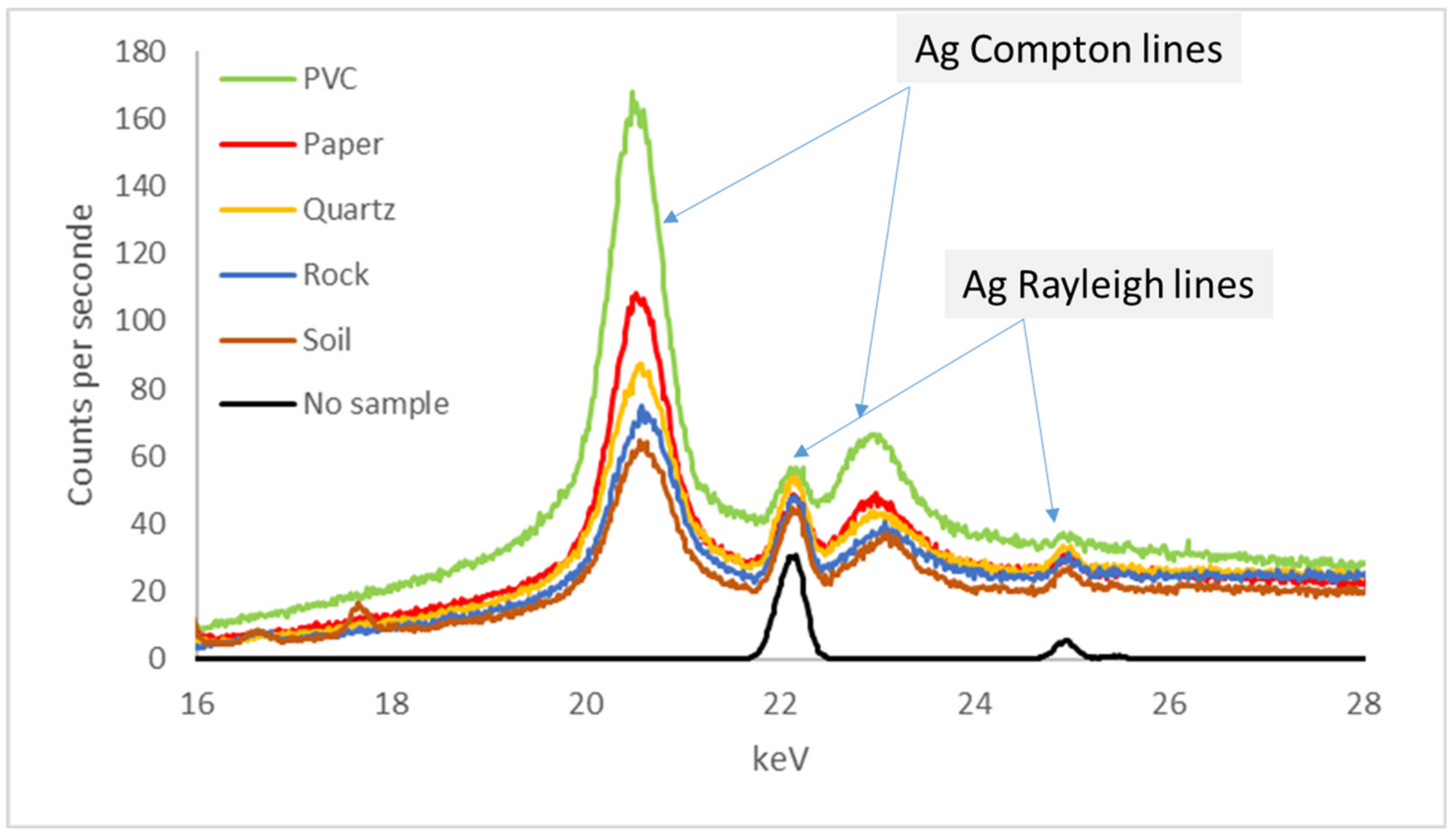
3.2.5. Effect of Films, Example 1

Sand-filled cups were covered by films of various nature (Figure 7). Analysis of the homogenised sand without film shows that the sand does not contain any P, and only a little Ca (400 mg/kg). Polypropylene films show little difference with filmless sample. On the other hand, analyses performed with Mylar™ films (TF-160-255) show ~3000 mg/kg P and ~1200 mg/kg Ca. Trace contamination levels of P and Ca were already observed in Mylar^® as for S [24]. The results of triplicate measurements performed in various film configurations illustrate the influence of film composition.

3.2.6. Effect of Films, Example 2

To overcome the problems caused by films, it is possible to use metal or plastic tubes with a diameter larger than that of the pXRF measurement windows (Figure 8). These tubes are filled with sample. The sample is then compacted in the pelletiser or in a press. This method provides compact samples with a flat, film-free surface between the sample and the spectrometer.

This parameter is important because the presence of a film of any composition (Mylar™, Prolene™ or polypropylene) greatly reduces the transmission of secondary X-ray fluorescence radiation for light elements.

This was investigated by performing triplicate measurements on a NIST600 bauxite standard sample with various membranes (4 or 6 µm) on the head of the device (Figure 4) and with various films (Prolene™ or Mylar™) on the sample (Figure 8 left), compared to a filmless tube (Figure 8 centre). Lighter elements are represented here by Si and Al, and heavier elements, by Fe.

The results of measurements (Figure 9a,b) illustrate the stronger influence of films on lighter elements than on heavier elements. For heavy elements like iron, the nature of the membrane or/and film or the number of films (1 or 2) has little or no influence and has very little impact on the detection of the element.

3.2.7. Effect of Films, Example 3 on Laterite Samples:

With the exception of Co, all the other elements see the slope of the ICP vs. pXRF regression line increase when a film is used, be it Kapton™, paper or PVC, the film attenuating the X-ray beam (primary and secondary,

Table 2. Relationship between laboratory and pXRF analyses using different films for sample packaging [32].

Lab XRF	pXRF	No Film	KaptonTM Film	Paper	PVC
Ni	Ni	Y = 1.26x	Y = 1.74x	Y = 1.62x	Y = 1.68x
Fe2O3	Fe	Y = 1.46x − 6.35	Y = 1.91x − 9.65	Y = 1.80x − 8.49	Y = 1.85x − 9.84
Co	Co	Y = 1.20x	Y = 0.74x	Y = 0.97x	Y = 1.19x
Cr2O3	Cr	Y = 2.37x	Y = 2.37x	Y = 2.39x	Y = 2.13x
Mn	Mn	Y = 1.07x	Y = 1.32x	Y = 1.31x	Y = 1.27x
SiO2	Si	Y = 2.06x	N/A	N/A	N/A
Al2O3	Al	Y = 1.5x + 1	N/A	N/A	N/A

N/A: Not applicable.

). An example for Ni is featured in Figure 10.

Kapton™ is sometimes coated with Co (cobalt-coated Kapton™), and although the composition of the material tested is not known, analysis of the data shows that the values are increased by a constant close to 0.16. If this value is subtracted from the data obtained with the Kapton™ film, the slope of the regression line goes from 0.74 to 2. It is therefore very likely that the materials tested contain more or less Co.

3.3. Light Element Analysis in pXRF

3.3.1. Difficulties Analysing Light Elements

Light elements (Z < 18) are difficult to measure by X-ray fluorescence for the following reasons (

Table 3. Energies (keV) of K and L lines [34].

Z	Symbol	Element	Kα	Kβ	Lα	Lβ	Lγ
12	Mg	Magnesium	1.25	1.30	-	-	-
13	Al	Aluminium	1.49	1.55	-	-	-
14	Si	Silicon	1.74	1.83	-	-	-
15	P	Phosphorus	2.02	2.14	-	-	-
16	S	Sulfur	2.31	2.46	-	-	-
17	Cl	Chlorine	2.62	2.82	-	-	-
18	Ar	Argon	2.96	3.19	-	-	-
19	K	Potassium	3.31	3.59	-	-	-
20	Ca	Calcium	3.69	4.01	0.34	-	-
21	Sc	Scandium	4.09	4.46	0.40	-	-
31	Ga	Gallium	9.24	10.26	1.10	1.12
32	Ge	Germanium	9.88	10.98	1.19	1.21
33	As	Arsenic	10.53	11.73	1.28	1.32
34	Se	Selenium	11.21	12.50	1.38	1.42
35	Br	Bromine	11.91	13.30	1.48	1.53
36	Kr	Krypton	12.64	14.11	1.59	1.64
37	Rb	Rubidium	13.38	14.97	1.69	1.75
38	Sr	Strontium	14.15	15.85	1.81	1.87
39	Y	Yttrium	14.95	16.74	1.92	2.00
40	Zr	Zirconium	15.77	17.68	2.04	2.12	2.30
41	Nb	Niobium	16.61	18.64	2.17	2.26	2.46
42	Mo	Molybdenum	17.48	19.63	2.29	2.40	2.62
43	Tc	Technetium	18.41	20.66	2.42	2.54	2.79
44	Ru	Ruthenium	19.28	21.66	2.56	2.68	2.96
45	Rh	Rhodium	20.21	22.75	2.70	2.83	3.14
46	Pd	Palladium	21.18	23.85	2.84	2.99	3.33
47	Ag	Silver	22.16	24.96	2.98	3.16	3.52
48	Cd	Cadmium	23.17	26.12	3.13	3.32	3.72
49	In	Indium	24.21	27.30	3.29	3.49	3.92

According to IUPAC, Kα = K − L₃, K − L₂; Kβ = K − M₂, K − M₃, K − M₄, K − M₅, K − N₂, K − N₃, K − N₄; Lα: L₃ − M₄, L₃ − M₅; Lβ = L₂ − M₄, L₃ − N₅, L₁ − M₃, L₁ − M₂, L₃ − O_4,5, L₃ − N₁, L₃ − O₁, L₃ − N_6,7, L₁ − M_4, L₁ − M_5, L₃ − N_4, L₂ − M₃; Lγ = L₂N₄, L₁ − N₂, L₁ − N₃, L₁ − O₃, L₁ − O₂, L₂ − N₁, L₂ − O₄, L₂ − O₁, L₂ − N₆₍₇₎.

):

• The fluorescence yield is very poor, as X-ray emission produces Auger electrons. In the Auger effect, an atom excited by ionisation, in the K layer for example, does not necessarily emit a photon of the K series outside the atom. Indeed, the emitted photon can be absorbed by the atom itself and expels a second electron from the upper layers (L, M, etc., in our example). This phenomenon is called the Auger effect and constitutes a non-radiative transition or internal conversion.
• The energy of the lines is low, so the photons are easily absorbed and generate a weak signal (Table 3).
• Light elements are only quantified from the K lines (lines 12 to 19 in Table 3), these are close to each other but also to the L lines of the heavier elements (lines 31 to 49 in Table 3). It is therefore difficult to distinguish them from each other. The energy resolution of pXRF devices is approximately 0.15 keV.
• In theory, on the basis of the energies of fluorescence (Table 1), the elements with atomic number Z < 20 should be considered as “light”. However, on the basis of the numerous studies published since 1995:
• Elements with Z < 12 cannot currently be analysed by pXRF, but only with state-of-the art laboratory equipment, or with another portable technique as LIBS [33];
• Elements with 18 < Z < 20 (K, Ca) are analysed in a generally satisfactory manner, despite the characteristics of their K lines. This is to be linked with their usual ranges, respectively 0.02 to 10% and 0.1 to 40%;
• Elements with 12 < Z < 18 exhibit significant difficulties and require high-performance devices and suitable preparation techniques. These are the elements that are the subject of this section.
• Light elements are, more than the others, subject to the phenomena of absorption of X-rays of fluorescence by air. On some devices, a light gas (usually helium) is used to purge the head of the device, which improves the quantification of light elements starting from the magnesium (Z = 12).

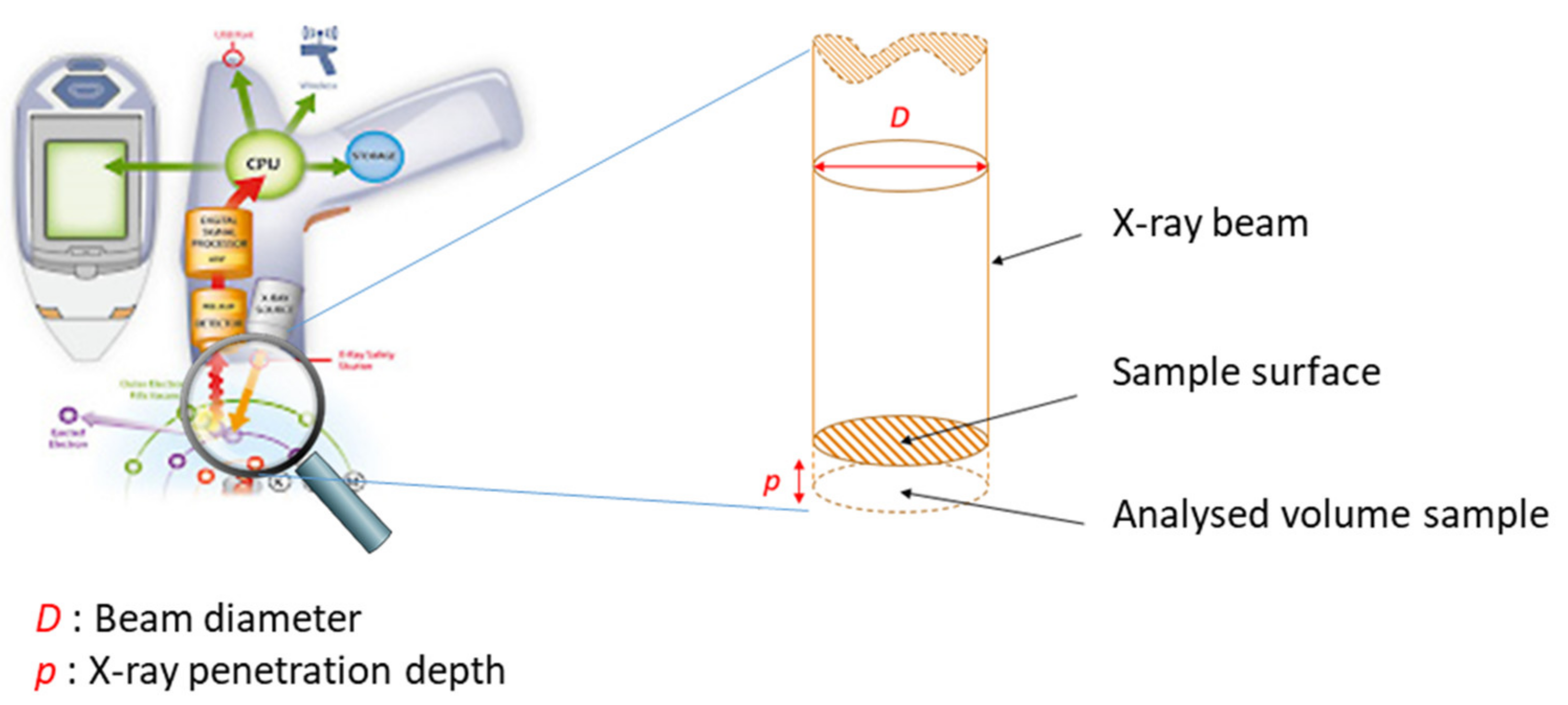
3.3.2. Geometry to Be Observed for Excitation of the Sample and Detection of X Photons

Depending on the device, the detectors are from 30 (sometimes less) to almost 70 degrees from the horizontal plane. A “thin nose” design is often chosen in order to approach the apparatus in difficult to access areas, with a higher angle of incidence as a result for portable spectrometers.

These devices are designed so that the axis of the detector and the axis of the tube converge at the same point. This point corresponds to the analytical distance at which the sample must be (working distance of the system). It is particularly critical when analysing elements of low energies such as Mg, Al, Si, P, and S.

Thus, spectrometers must always be in contact with matter, not at a distance from it. However, the material must not enter the circular hole of the analyser, the depth of which is equal to the thickness of the front plate, because in this case the focal distance to the detector becomes too short.

Indeed, when working on powdery materials without protecting the nose of the device with the mask (metal plate with a Kapton window, see Figure 5 in Section 3.2.2), material enters the circular hole of the analyser. If there is any powder in this area, the analytical distance at which the sample is located is shorter than it should be, and the measured values are probably overestimated.

Moreover, this hole is only separated from the detection chamber by a very thin window made of fragile polymer (see Section 3.2). In addition to the risk of costly damage in the event of this window breaking, the accumulation of sample remains around the window will lead to cross contamination between measurements.

3.3.3. Geometry to Be Respected for the Analysis of Light Elements

When analysing light elements, the front plate with Kapton™ membrane should not be used, the latter being too absorbent. To be able to use the spectrometer without protection, the sample must be more or less consolidated. The following techniques can be used for powdery materials (Figure 8):

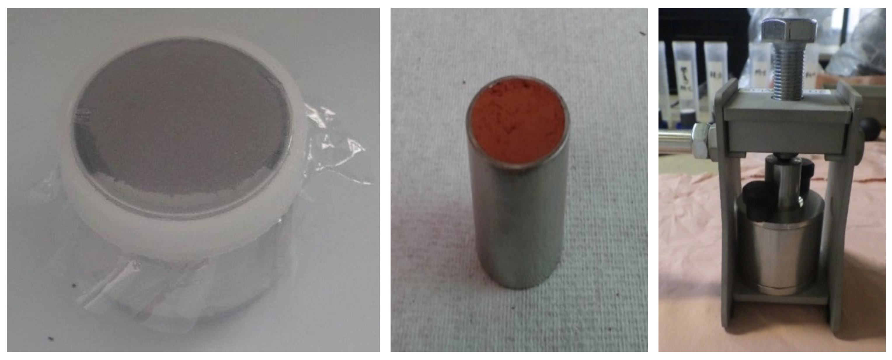
• pelletising with a hammer shock tube,
• pelletising with the press, possibly with the addition of a binder, kaolin, talc, or wax,
• compacting the surface of the material and measuring over it, the nose of the device simply placed, without pressing.

In the latter case, it is possible to apply a 4 µm Prolene™ film to the nose of the device, in order to protect the measurement window.

3.3.4. Other Points to Observe for the Analysis of Light Elements

If the sample is crystallised or partially crystallised, an X-ray diffraction phenomenon will essentially disturb the measurement of the lines of light elements since these will be partly offset.

The analysed depth will be much thinner than for heavier elements. This implies that

• For a low energy line with a shallow penetration depth, the surface layer must therefore be representative of the sample, which makes sample preparation critical (this problem being similar to that of sampling);
• For a very energetic line, which penetrates deeper, the received signal is an average over a large volume, but if the sample is too thin, the hypothesis of “infinite thickness” is no longer valid, and there may be interference from the bottom support material.

3.4. Analytical Interferences in pXRF, and Taking Them into Account in Geochemical Investigations

3.4.1. Principle

The interference encountered in X-ray fluorescence spectrometry has been known for a long time [35,36,37,38], the main ones being due to

• Physical effects of the matrix (particle size, homogeneity, surface effect);
• Humidity and porosity of the sample;
• Chemical effects of the matrix (decrease or increase in the intensity of a line of an element caused by the presence of another element);
• Interference between the Kα/Kβ lines;
• Interference between the K/L, K/M and L/M lines.

The Pb-As interference is described in [39], where it is mentioned that this interference is partly corrected by the spectrometers’ software but prevents any reliable As analysis when Pb/As is >10. The Fe-Co interference is also documented [40].

The software integrated in the X-ray fluorescence spectrometer takes into account the interferences between the different chemical elements for the calculation of the contents, but it does not always compensate for them all, and the contents of some of these elements may be under- or overestimated compared to the real contents.

Even if the X-ray fluorescence device has an internal calibration and it is possible to test the device with NIST or other reference samples, the manufacturers recommend using a limited number of reference samples from the same study site as those analysed by X-ray fluorescence and having a comparable matrix. These will be analysed by usual chemical analysis methods (ICP-AES or MS spectrometry) and will be used to establish the calibration curves between the ICP data and the X-ray fluorescence data. Thus, the effects linked to the matrix will be the same.

3.4.2. Chemical Effects of the Matrix

Some matrix effects are chemical, that is, they only involve the elemental composition of the sample. In the case of XRF, they involve two phenomena: absorption and secondary fluorescence.

The intensity of a line is not proportional to the element content, because the other elements constitutive of the sample modify the signal.

Matrix Effect: Absorption

The signal level depends on the absorption of X-rays by the sample before they reach the target atom: It is called the absorption effect. The characteristic X-rays of element 1 are partly absorbed by element 2 which decreases its signal without element 2 being detected (Figure 11). An example of Zn signal absorption by Fe is given by [19].

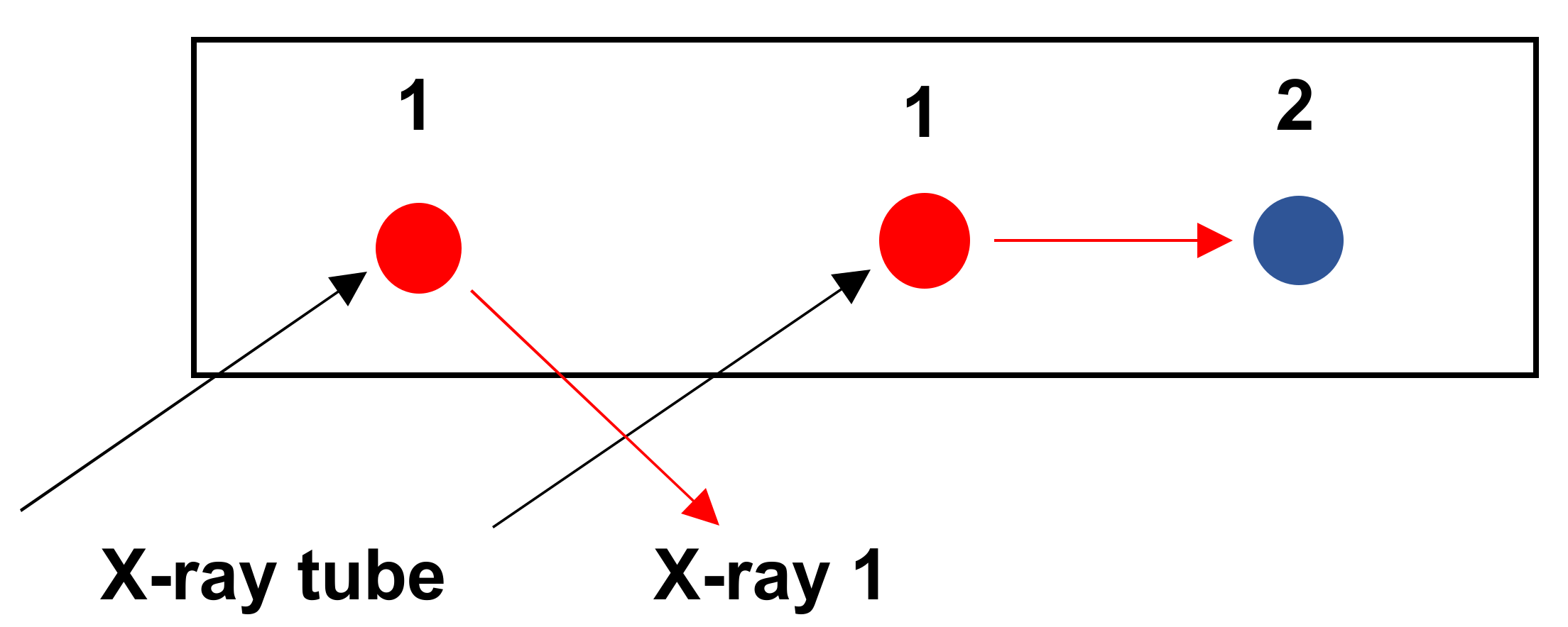
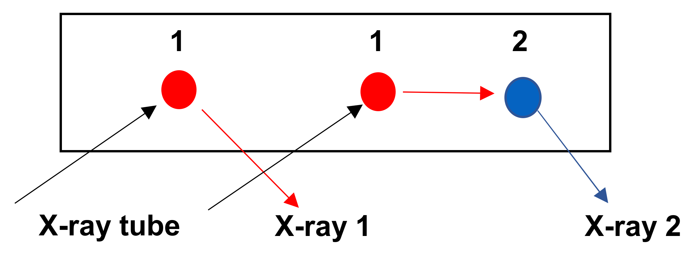
Matrix Effect: Excitation

Secondary absorption plays a role on the radiation resulting from X-ray fluorescence between the target atom and the surface of the sample. Secondary fluorescence, or overexcitation, designates the excitation of a neighbouring atom by secondary X-rays. The atoms in the sample therefore receive X-rays from the tube and X-rays from other atoms (Figure 12).

3.4.3. Interference between K /Kβ Lines

In the case of Kα/Kβ interferences, these appear when the line Kβ of an element Z-1 overlaps the line Kα of the element Z (

Table 4. Potential Kα/Kβ interferences (keV) [34].

eV	Line	Interferent	Distance (eV)	Reference
4090.6	21 Sc Kα1	20 Ca Kβ1	78
5414.72	24 Cr Kα1	23 V Kβ1	13
5898.75	25 Mn Kα1	24 Cr Kβ1	48
6490.45	25 Mn Kβ1	26 Fe Kα1	5	[40]
6930.32	27 Co Kα1	26 Fe Kβ1	128	[40]

). The intensity of the ratio Kα/Kβ is generally from 7/1. If the element Z-1 is present in the sample in much larger quantities than element Z, it will be difficult to determine the concentration of the latter. One of the most common interferences in soils is that between iron and cobalt. The iron content is generally several % while Co contents is below 100 mg kg⁻¹. With the current resolution (resolution between two lines, of the order of 150 eV on the XL3t980 and 380 eV on the XLt723), it is practically impossible to measure Co in soils because the latter is systematically and largely overestimated.

3.4.4. Interference between K/L, K/M and L/M Lines

In the case of the interferences between the lines K/L, K/M and L/M, these appear when, for example, the line Kα of an element 1 overlaps the line Lα of an element 2 (

Table 5. Potential K/L, K/M and L/M interferences (keV) [34].

eV	Line	Interferent	Distance (eV)	Reference
3443.98	50 Sn Lα1	19 K Kα1	130
3604.72	51 Sb Lα1	20 Ca Kα1	87
4466.26	56 Ba Lα1	22 Ti Kα1	45
4650.97	57 La Lα1	22 Ti Kα1	140
6403.84	26 Fe Kα1	REE L peaks		[34]
10551.5	82 Pb Lα1	33 As Kα1	8	[40]

). To determine the exact concentration of elements 1 and 2, it is possible to use the Kβ and Lβ lines of these same elements. By using lower intensity lines, the device loses sensitivity.

The integrated software can take account of these interferences, but if the ratio between elements 1 and 2 is greater than 10, the mathematical correction will not correctly determine the content of element 2 in the presence of high contents of element 1.

The relationship between the lines of the same pure element is known, but unfortunately is not always constant, depending on the density of the matrix. In addition, the deconvolution is based only on the height of the peak (strip in the centre), not on its shape (which would be more precise with a deconvolution of line profile).

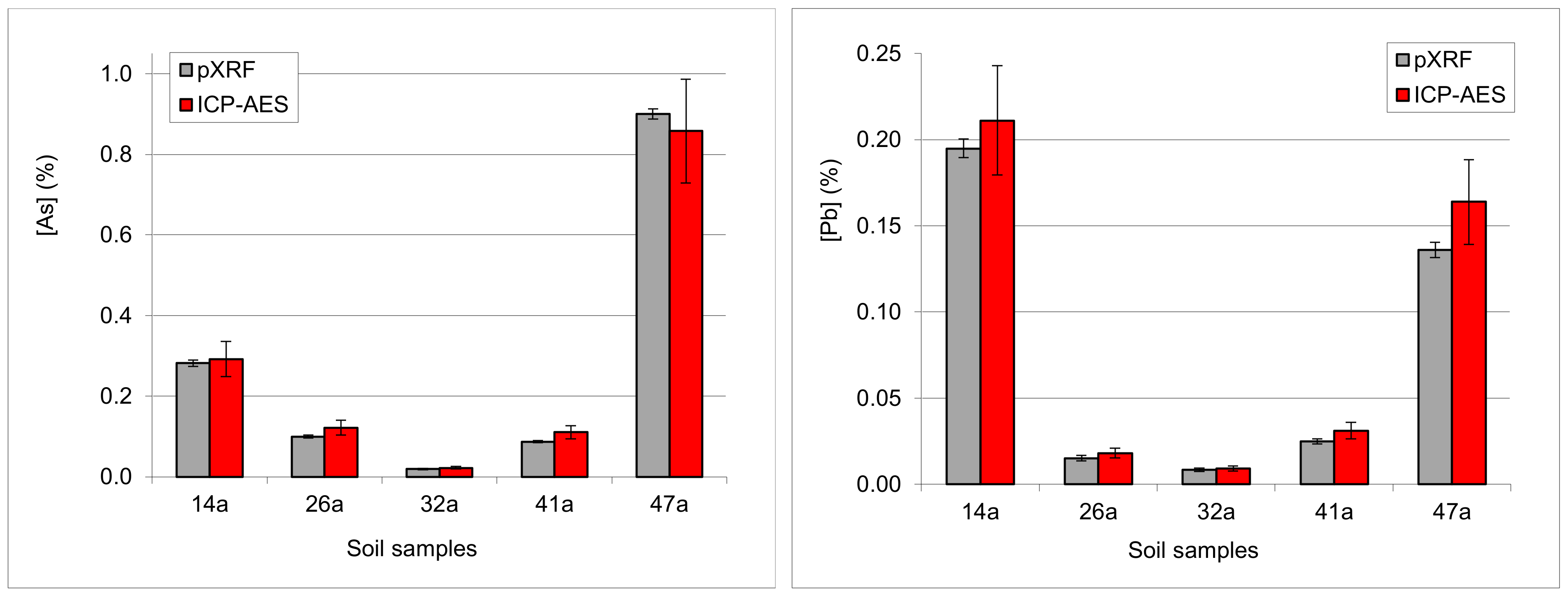
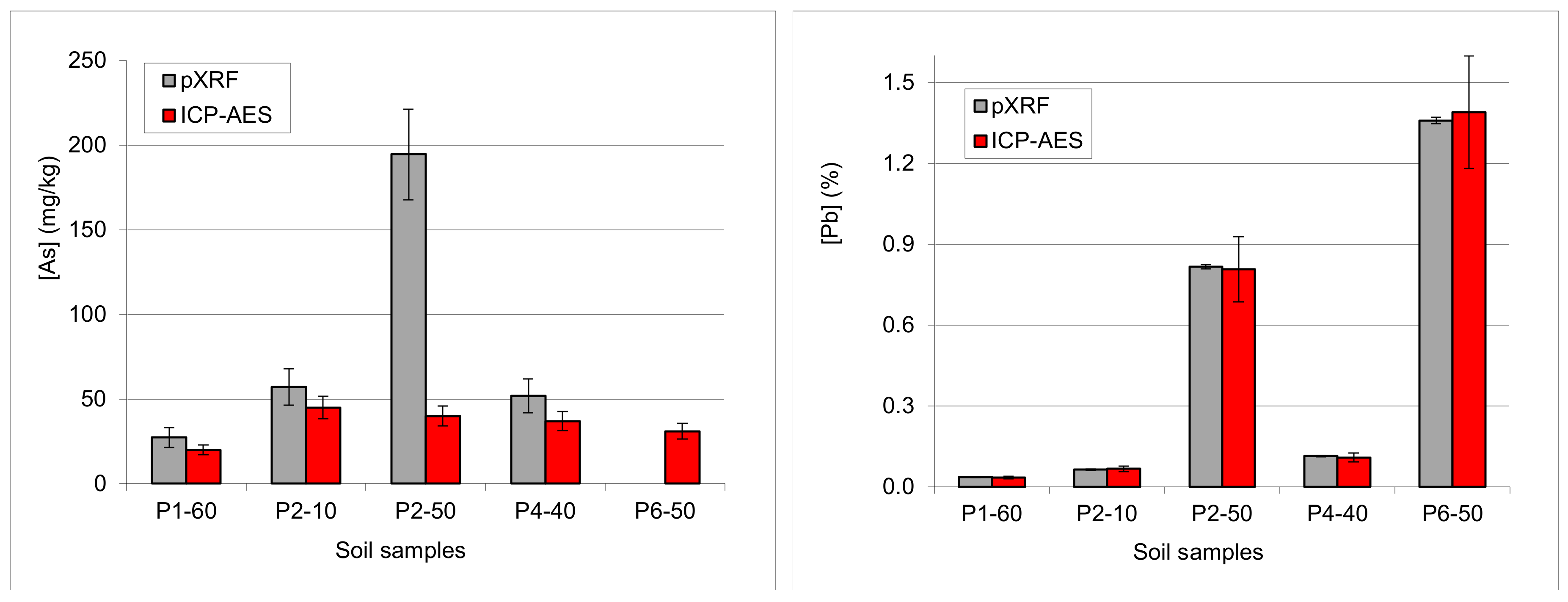
3.4.5. Examples: As-Pb Interference

When the As contents is higher or of the same order as the Pb contents, the As contents is correctly quantified (Figure 13).

When the As contents is lower than the Pb contents (Pb/As ratio >10), the As contents is either not quantified or overestimated (Figure 14).

As pXRF spectrometers calculate the measurement uncertainty separately for each sample, as a function of the matrix, and deduce a LOD (limit of detection, or lower analytical limit), it can be noted that the LOD for As increases as Pb increases.

3.5. Physical Effects of the Matrix

pXRF analysis is carried out on a very small volume of material, limited by the small size of the measurement window (<1 cm²) and the X-ray beam’s focusing and low penetration (generally between 0.1 and 1 mm, sometimes less). This is a volume analysis, unlike wet laboratory techniques, which are based on mass. The concentrations by pXRF are indeed expressed in mass proportions (mg/kg) but are calculated from the number of analyte atoms present in a given volume, regardless of density.

It is foreseeable that the physical nature of the sample (particle size, porosity, humidity, etc.) will affect the pXRF measurement and cause it to deviate from a wet chemical analysis of the same sample with a well known preparation even if the analytical conditions of the pXRF measurement are perfectly rigorous.

The majority of users expect pXRF to have the same results as an XRF laboratory device. This can be achieved for equal preparation, but this is not usually possible under on-site conditions. Correlation of field results with the laboratory has to be verified later, after suitable preparation. We recommend analysing the pulps with the pXRF, after laboratory preparation and analysis, to be able to distinguish between sample preparation bias and analytical bias.

Note also that instruments are factory calibrated for powders, for their Fundamental parameters (Mining, Geochem) and Compton (Soil) modes. This may lead to positive bias when samples are pelletised.

3.5.1. Physical Effects of the Matrix (Homogeneity, Particle Size, and Surface Effect)

Because of the weak penetration power of X-rays, generally only the first layers of the particles are analysed. It is therefore essential that all of these layers are as homogeneous and representative as possible. In addition, the size of the pXRF window is only 8 mm, so the analysed area is limited. Depending on the type of device used, the volume analysed ranges between 0.01 cm³ and 0.02 cm³, a sample mass of the order of a few tens of milligrams (Figure 15).

The intensity of the X-rays emitted varies significantly depending on the particle size distribution. Despite all the care taken in grinding, this phenomenon cannot be avoided. On large grains, X-rays give information on the specific composition of the elements contained in these grains, while on small particles the information received will be representative of the general composition.

In addition, when grains are large, the X-rays emitted are partially reabsorbed, which can in some cases be completely absorbed (opacifying effect). The sensitivity of the spectrometer varies depending on the distance between the X-ray tube and the sample. The flatness of the preparation should therefore be as perfect as possible. The effect is greatest on light elements up to potassium (K).

3.5.2. Effects of Moisture in Fine-Grained Samples

The presence of water in a sample results in a first approach by dilution and attenuation of the signal. The contents of the elements will be inversely proportional to the humidity, and the detection limits will increase in proportion. However, this proportionality is only approximate. In addition, the coefficient applicable to the contents varies according to the elements (the heavy ones are less affected than the light ones) and the composition of the matrix (more or less absorbent).

Researchers noticed early that moisture in a sample significantly affects pXRF measurements but accepted that moisture below 20% [39,41,42] or even 30% [43] was still acceptable. A correction scheme was proposed by [44,45]. Further research demonstrated that on-site dehydration by a hand-operated press [17] allowed useful measurements on wet sediment, soil or waste up to 50% moisture, and maybe more. The first effect of moisture is to dilute the analytes in a larger volume, roughly proportional to the water contents. The resulting dilution effect is counterbalanced by a reduced matrix absorption. Measurements performed at variable stages of sample drying (Figure 15) show that it is possible to estimate Pb, Zn, and Cu dry concentrations from measurements on samples with water contents of between 25% and 50% (Figure 16) by correcting linear biases [10,17,43,46]. This not really bias, as water is actually part of the sample in the field [47] but it is often interpreted as such when comparing with laboratory analyses. These biases are element specific, and stronger for light elements than for heavier ones [17,42]; hence, dependent on the matrix composition [41]. Measurements on partially dehydrated wet samples can be used for decision-making during field operations, for sample ranking or for laboratory screening. Although the ranking of samples in terms of concentration remains correct, even with water contents >50%, the slope itself varies from element to element. Despite differences between elements, biases do not mask the geochemical signature [48]. Linear corrections were proposed by [49] but they need to be further refined using laboratory analyses.

3.5.3. Moisture and Grain Size

Adding water to a sample has the effect of absorbing partly X-rays. This alters the response of all the elements, but not with the same amplitude: the secondary fluorescence X-rays of the light elements are more absorbed than those of heavy elements. At first, the contents of the elements will be inversely proportional to the humidity. The addition of water to a porous sample has a dilution effect on the atoms of the sample. It is indeed a volumic effect and not a mass dilution. If there are fewer atoms in the volume explored by X-rays because of the volume of added water, the response of the atoms will be decreased, and the quantification will be elements will be underestimated. In a second step, beyond a large water contents, it will no longer be possible to detect certain elements because the water will completely absorb the secondary fluorescence X-rays of these elements especially light elements.

A given amount of added water will not be distributed evenly in the sample, depending on the grains’ size and wettability. If the grains are not wettable, water will be drained down to the bottom of the sample. If the grains have high wettability, water will form a layer around the grains. The thickness of the film depends on the grain size, the wettability, and the amount of water. By introducing water, the interstices are filled. The interstitial volume depends on the grains’ size and plasticity. Depending on the distribution and amount of water in the sample, the response of the elements will be more or less affected, but not with the same amplitude. It is therefore important to know or control the humidity rate (see Section 3.5.5).

The use of pressed pellets was found by [50] to be superior to any form of loose sample, and to give closest results to laboratory XRF. With this technique the spectrometer can be operated without any sample protection film while reducing issues with porosity, grain size, and sample density.

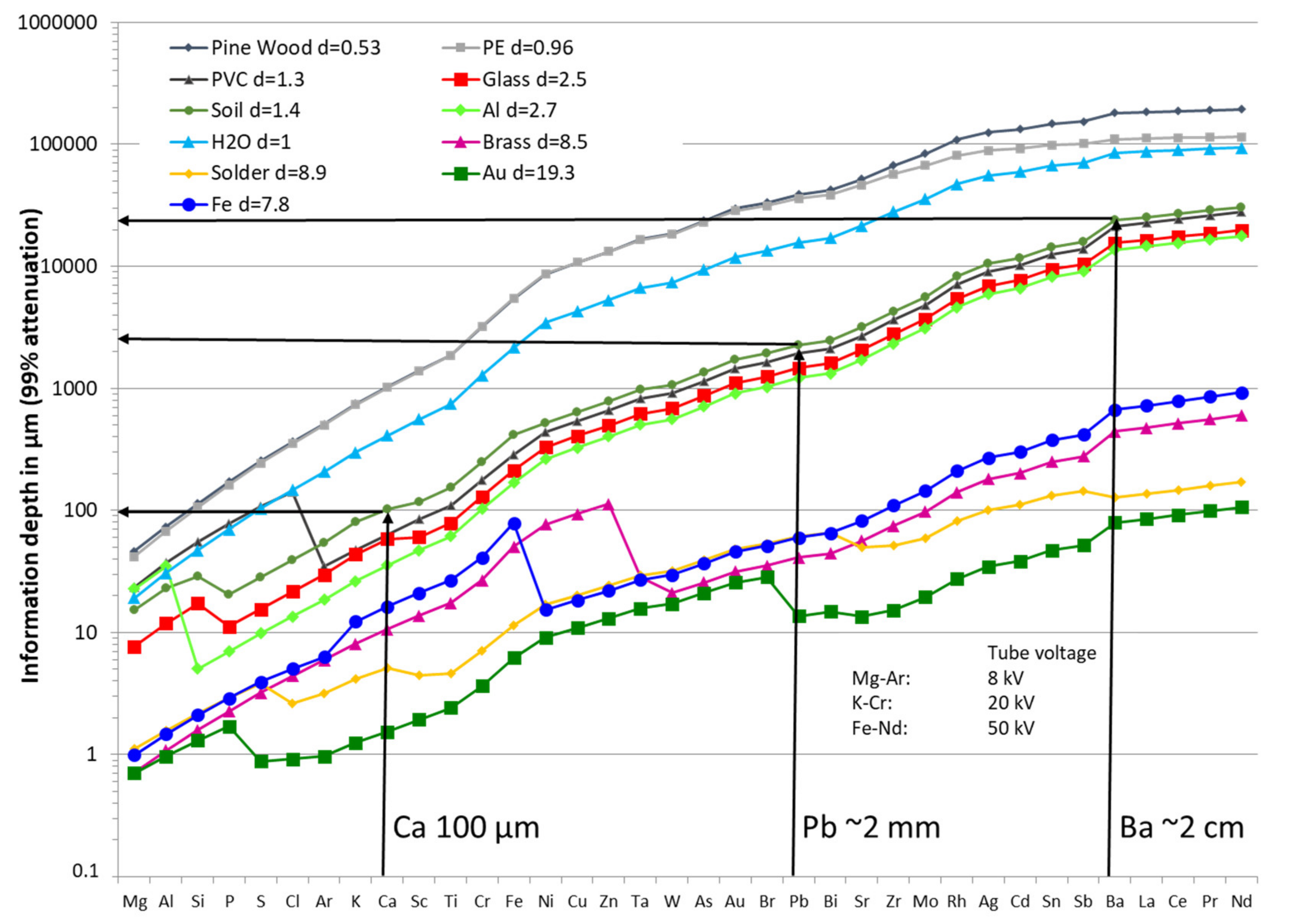
3.5.4. Depth of Analytical Investigations

Most pXRF users are not fully aware of the physical phenomena surrounding pXRF analysis. For instance, the penetration depth of the primary X-rays should not be confused with the absorption depth of secondary X-rays. The latter is shallower than the former and is dependent on the element analysed. This affects both the minimum sample thickness (the primary rays should not be able to reach the underlying material, such as a metal pan) and the part of the sample actually analysed (thinner for the lighter elements).

It is therefore important to explain the “information depth” variable (Figure 17) to pXRF users who are not XRF specialists. Indeed, this diagram clearly shows the difference between the depth of penetration of primary radiation and the “thickness” of sample matrix from which the secondary radiation specific to each element will come back to the detector. For a soil matrix, 99% of the response of Ca is given by the first 100 µm of the sample, while for Pb, 99% of the response is given by the first 2 mm, and for Ba, 99% of the response is given by 2 cm. So, if the sample is only 1 cm thick, Ca and Pb will be properly quantified, while Ba will be underestimated. Hence, the notion of infinite thickness. Overall, insufficient sample thickness can cause inaccurate measurements below 10 mm, depending on the element [46].

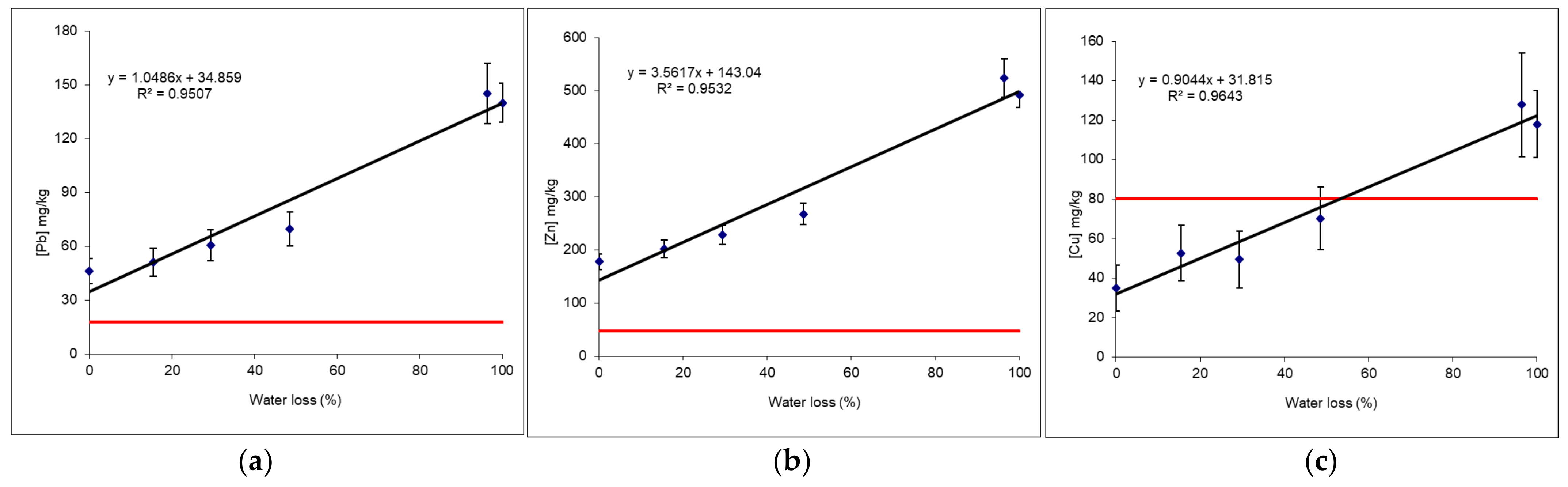
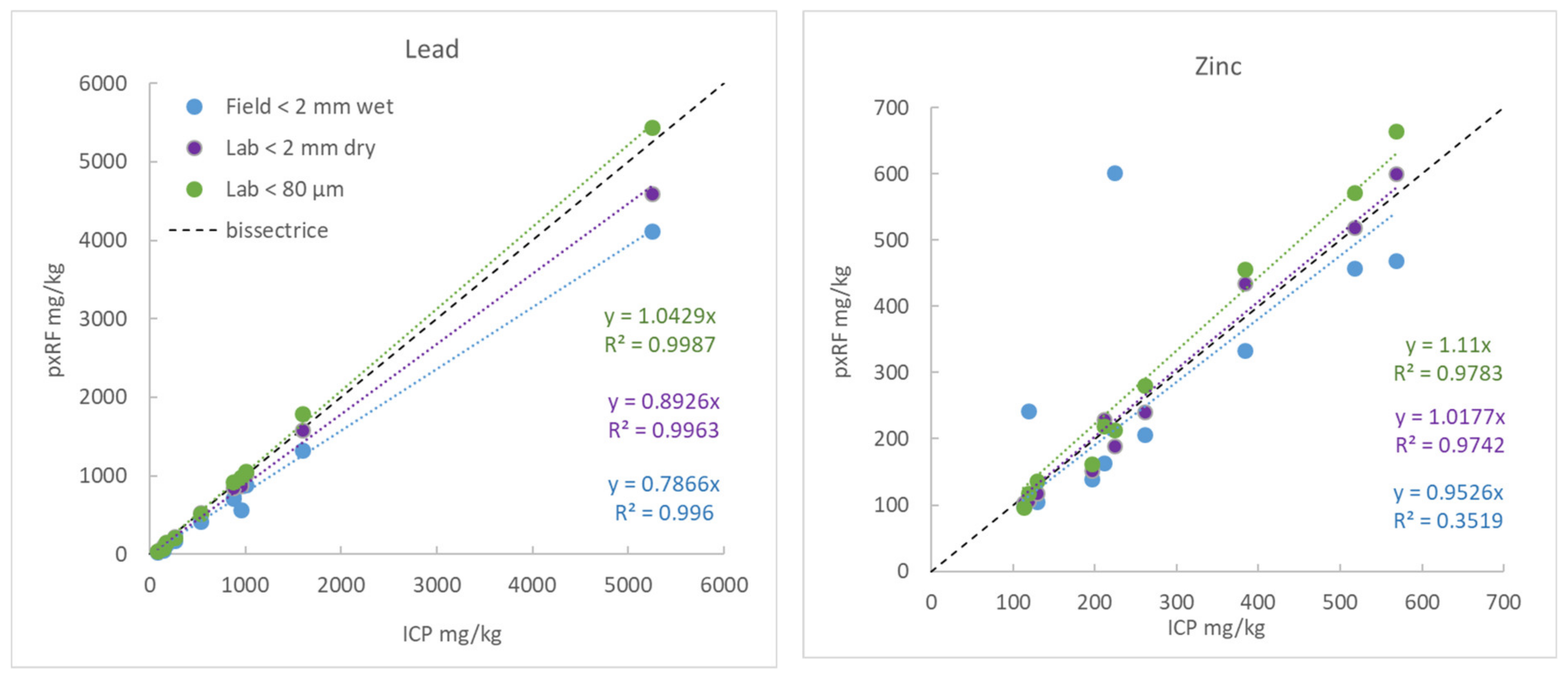
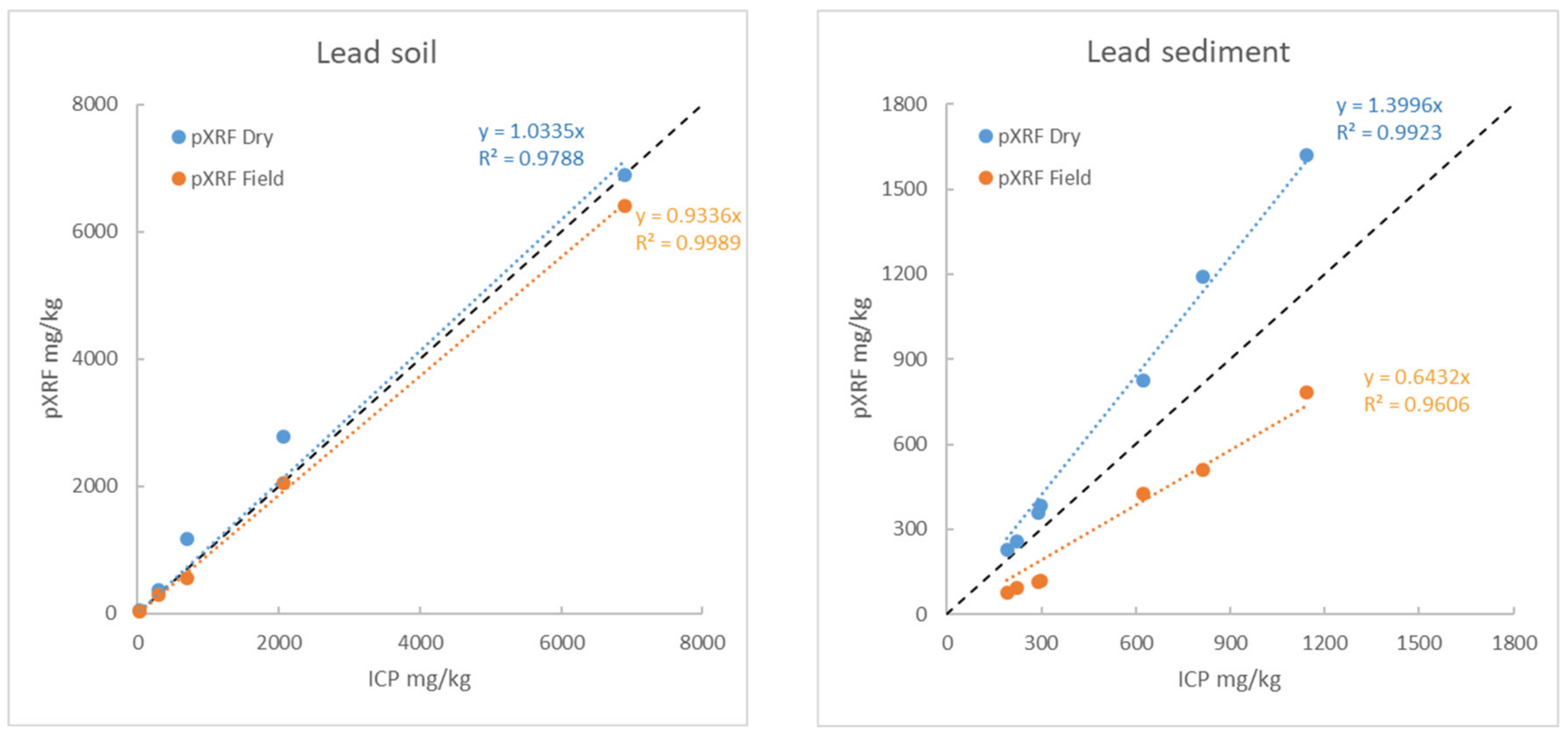
3.5.5. Example 1: Behaviour of Pb and Zn as a Function of Humidity and Article Size

The results of analyses of ten samples of polluted soils with different preparations were compared for lead and zinc. The ICP/AES analyses were compared to the pXRF analyses obtained on three different preparations (Figure 18):

• Raw samples, that is to say sieved to 2 mm but still wet (measurements on-site “Wet ground” with an average humidity rate of 20%),
• Raw samples, that is to say sieved to 2 mm and dried in a lab oven at 40 °C (“Lab < 2 mm dry”),
• Samples dried and ground to 80 µm (“Lab < 80 µm”).

Whatever the preparation, Pb measurements by pXRF are well correlated with the ICP analyses (0.9960 < r² < 0.9987) and the contents determined by pXRF increases with the care taken in preparing the samples:

“Wet ground” < “Lab < 2 mm dry” < “Lab < 80 µm”

Unlike Pb, the results for Zn are not always very well correlated with the ICP results depending on the preparation (r² = 0.3519 for samples in the field). The correlations are clearly improved when the samples are homogenised after drying at 2 mm and/or after grinding at 80 µm (r² > 0.97).

These results show the importance of sample preparation. In this example, Pb and Zn are not distributed in the same way in or on the particles. Pb is distributed in a homogeneous manner, while Zn is not. Sieving a sample in the field to <2 mm clearly improves XRF measurements and make it possible to limit routine analyses to a single measurement. However, this may be not sufficient on some samples, and that it is sometimes necessary to make several measurements on the sieved sample.

3.5.6. Example 2: Impact of Density on the Measurement

The analysis of freshly sampled surface sediments by pXRF is difficult because of the significant quantity of water in the samples (ranging from 30% to 70%), it is not possible to analyse them directly. Using a sediment press (Figure 19), it is possible to prepare pellets, containing less water and above all to obtain sediments with similar water contents from one sample to another and thus to be able to compare the measurements. Once dried, these pellets become extremely hard and very compact (similar to concrete). The analysis of these dry pellets shows very different behaviour than the result on soils. Indeed, for soils, the slope of the correlation line is around one on dry samples, while for sediments whose average water content is initially 48%, the slope goes from 0.64 to 1.40 on the dried pellets. The “soil” mode is designed for powder samples with an average density of 1.8, this order of magnitude must always be respected. By drying the pellets in the oven (water range from 0 to 3%), the apparent density was increased, and an overestimation of the measured contents was observed.

3.5.7. Other Potential Issues with pXRF

This section comprises issues that should be kept in mind by the user but are already dealt with by suitable references.

Operating many devices, comparing their measurements and consolidating data tables: This happens when a project uses several instruments that are different models or brands. Calibration curves are usually specific to each instrument, and bias varies across instruments. It is not recommended to merge results without cross-checking them instrument by instrument with a single reliable source of laboratory analyses [10]. Errors may happen also while consolidating tables, as the sequence of elements varies from brand to brand, and even from mode to mode (Niton).

Analysis time has to be adjusted for each filter prior to operations, taking into account the precision objectives and the instrument’s performance. Most modern instruments can be operated with 15 to 30 s per filter, with a total analysis time per mode between 30 and 90 s. Precision and sensitivity are improved by a longer analysis time, above which no improvement is observed. The above durations are optimal compromises for field use [10,11,20,26,51], while longer durations require a bench.

The operating temperature of the detector area needs to be stabilised for accurate readings [40,52], and it is recommended to allow at least 15 min for pre-heating before performing measurements or CRM checking. However, it is possible to perform qualitative measurements during pre-heating, as element ratios are less affected.

A time drift can be observed with a given instrument [11], and this may require a periodic factory calibration if absolute accuracy is expected. Battery life affects measurements [10,53]. It is recommended to replace a battery when below 25% charge, or to perform qualitative measurements only with the remaining charge. Weather and elevation issues are known to affect accuracy through barometric pressure variations [53].

4. Discussion

The use of inappropriate thicker spectrometer windows or of film covers on samples will lead to bias of varying significance, mainly underestimation, on mid-range elements (K to Se), and unpredictable absorption on lighter elements (Al to S). Heavier elements are usually less affected. The common practice of shooting through sample bags may lead to the same effects, but it does not affect sample ranking by element concentration or element signatures. According to this, the use of measurements in sample bags is widely accepted in exploration and is acceptable as long as the main objective is mapping or vectoring.

Light element analysis is often advertised by instrument manufacturers as a straightforward process, but very few papers document this possibility. Most light element studies carried out with pXRF [21,54] are actually made on pressed pellets (or other uncovered samples). The use of a light hand press or a hammer-operated tube can be slightly time consuming but is manageable while on-site.

Overlooking potential analytical interferences will usually lead to poor correlation between pXRF and laboratory analyses. In most papers, such results are usually skipped, and the user may disseminate the statement that “this spectrometer does not analyse properly this element”. More generally, the “black box” approach of most manufacturers (reporting only corrected results through the instrument’s software) leads to the general belief that pXRF results can replace laboratory analyses without any chemist’s skills. Overlooking the matrix effects of the physical properties of samples will usually lead to the same conclusions as those stated above on films: as long as all samples have similar physical properties, the result may be a general bias and have little effect on sample ranking. This is no longer true when physical properties vary. A simple example can be designed from soil analyses performed on rainy days after dry days. Dry soil samples can be sieved, homogenised and densified—ready for reproducible analyses—while wet soil samples have to be analysed in their raw state, with a high moisture rate, or to be dried and processed later at the camp. Mixing both types of measurements in a map will lead to strongly erroneous patterns.

5. Conclusions

Measurements performed on-site with a pXRF cannot match the accuracy of state-of-the-art laboratory analyses, as both instrument construction and sample preparation include compromises for the needs of mobility. However, they can approach laboratory quality if the same level of attention is given to careful sample preparation and to appropriate quality procedures. Paying attention to the potential pitfalls and issues we have examined will further improve the quality of on-site measurements and prevent big mistakes.

Measurements performed with simplified procedures may provide useful results too, even if these procedures incorporate significant biases in results. Biases will not affect sample concentration ranking or spatial distribution. This will allow dynamic sampling, laboratory sample selection and decision making on-site. Furthermore, on-site measurements will significantly improve the representativity of laboratory samples, by reducing heterogeneity issues at the media level [21].

We believe that strong understanding of pXRF characteristics is required to avoid reporting erroneous results. With this caveat, using pXRF on-site can produce valuable field data sets and improve the quality and relevance of laboratory data sets.

References

1. Gałuszka, A.; Migaszewski, Z.M.; Namieśnik, J. Moving your laboratories to the field—Advantages and limitations of the use of field portable instruments in environmental sample analysis. Environ. Res. 2015, 140, 593–603. [Google Scholar] [CrossRef] [PubMed]
2. Hu, W.; Huang, B.; Weindorf, D.C.; Chen, Y. Metals Analysis of Agricultural Soils via Portable X-ray Fluorescence Spectrometry. Bull. Environ. Contam. Toxicol. 2014, 92, 420–426. [Google Scholar] [CrossRef] [PubMed]
3. Sharma, A.; Weindorf, D.C.; Wang, D.; Chakraborty, S. Characterizing soils via portable X-ray fluorescence spectrometer: 4. Cation exchange capacity (CEC). Geoderma 2015, 239–240, 130–134. [Google Scholar] [CrossRef]
4. Lemière, B. A review of applications of pXRF (field portable X-ray fluorescence) for applied geochemistry. J. Geochem. Explor. 2018, 188, 350–363. [Google Scholar] [CrossRef] [Green Version]
5. Tighe, M.; Rogan, G.; Wilson, S.; Grave, P.; Kealhofer, L.; Yukongdi, P. The potential for portable X-ray fluorescence determination of soil copper at ancient metallurgy sites, and considerations beyond measurements of total concentrations. J. Environ. Manag. 2018, 206, 373–382. [Google Scholar] [CrossRef] [PubMed]
6. Weindorf, D.C.; Bakr, N.; Zhu, Y. Advances in Portable X-ray Fluorescence (PXRF) for Environmental, Pedological, and Agronomic Applications. Adv. Agron. 2014, 128, 1–45. [Google Scholar] [CrossRef]
7. Ravansari, R.; Wilson, S.C.; Tighe, M. Portable X-ray fluorescence for environmental assessment of soils: Not just a point and shoot method. Environ. Int. 2020, 134, 105250. [Google Scholar] [CrossRef]
8. Kilbride, C.; Poole, J.; Hutchings, T. A comparison of Cu, Pb, As, Cd, Zn, Fe, Ni and Mn determined by acid extraction/ICP–OES and ex situ field portable X-ray fluorescence analyses. Environ. Pollut. 2006, 143, 16–23. [Google Scholar] [CrossRef]
9. Radu, T.; Diamond, D. Comparison of soil pollution concentrations determined using AAS and portable XRF techniques. J. Hazard. Mater. 2009, 171, 1168–1171. [Google Scholar] [CrossRef]
10. Hall, G.; Buchar, A.; Bonham-Carter, G. Quality Control Assessment of Portable XRF Analysers: Development of Standard Operating Procedures, Performance on Variable Media and Recommended Uses. Canadian Mining Industry Research Organization (CAMIRO) Exploration Division, Project 10E01 Phase I Report. 2012. Available online: https://www.appliedgeochemists.org/index.php/publications/other-publications/2-uncategorised/106-portable-xrf-for-the-exploration-and-mining-industry (accessed on 17 December 2013).
11. Bourke, A.; Ross, P.-S. Portable X-ray fluorescence measurements on exploration drill-cores: Comparing performance on unprepared cores and powders for ‘whole-rock’ analysis. Geochem. Explor. Environ. Anal. 2015, 16, 147–157. [Google Scholar] [CrossRef] [Green Version]
12. Rouillon, M.; Taylor, M.P. Can field portable X-ray fluorescence (pXRF) produce high quality data for application in environmental contamination research? Environ. Pollut. 2016, 214, 255–264. [Google Scholar] [CrossRef] [PubMed]
13. Young, K.; Evans, C.A.; Hodges, K.V.; Bleacher, J.E.; Graff, T.G. A review of the handheld X-ray fluorescence spectrometer as a tool for field geologic investigations on Earth and in planetary surface exploration. Appl. Geochem. 2016, 72, 77–87. [Google Scholar] [CrossRef] [Green Version]
14. Laperche, V.; Hammade, V. Diagnostic Rapide sur site—Utilisation de Méthodes D’évaluation de la Teneur en Métaux de sols Pollués par Mesure de leur Susceptibilité Magnétique et par Fluorescence X; Report CNRSSP/02/08; CNRSSP: Douai, France, 2002. [Google Scholar]
15. Laperche, V. Evaluation des Performances du Spectromètre Portable de Fluorescence X Niton XL723S (au Laboratoire et sur le Terrain). BRGM Report RP-53377-FR. 2005, 72p. Available online: http://infoterre.brgm.fr/rapports/RP-53377-FR.pdf (accessed on 23 December 2020).
16. Liakopoulos, A.; Lemière, B.; Michael, K.; Crouzet, C.; Laperche, V.; Romaidis, I.; Drougas, I.; Lassin, A. Environmental impacts of unmanaged solid waste at a former base metal mining and ore processing site (Kirki, Greece). Waste Manag. Res. 2010, 28, 996–1009. [Google Scholar] [CrossRef] [PubMed]
17. Lemiere, B.; Laperche, V.; Haouche, L.; Auger, P. Portable XRF and wet materials: Application to dredged contaminated sediments from waterways. Geochem. Explor. Environ. Anal. 2014, 14, 257–264. [Google Scholar] [CrossRef] [Green Version]
18. Quiniou, T.; Laperche, V. An assessment of field-portable X-ray fluorescence analysis for nickel and iron in laterite ore (New Caledonia). Geochem. Explor. Environ. Anal. 2014, 14, 245–255. [Google Scholar] [CrossRef]
19. Parsons, C.T.; Grabulosa, E.M.; Pili, E.; Floor, G.H.; Román-Ross, G.; Charlet, L. Quantification of trace arsenic in soils by field-portable X-ray fluorescence spectrometry: Considerations for sample preparation and measurement conditions. J. Hazard. Mater. 2013, 262, 1213–1222. [Google Scholar] [CrossRef]
20. Markowicz, A.A. Quantification and Correction Procedures. In IAEA, In Situ Applications of X Ray Fluorescence Techniques; IAEA-TECDOC-1456 (ISBN:92-0-107105-1). 2005. Available online: http://www-pub.iaea.org/books/IAEABooks/7212/In-Situ-Applications-of-X-Ray-Fluorescence-Techniques (accessed on 15 September 2014).
21. Adams, C.; Brand, C.; Dentith, M.; Fiorentini, M.L.; Caruso, S.; Mehta, M. The use of pXRF for light element geochemical analysis: A review of hardware design limitations and an empirical investigation of air, vacuum, helium flush and detector window technologies. Geochem. Explor. Environ. Anal. 2020, 20, 366–380. [Google Scholar] [CrossRef]
22. Ravansari, R.; Lemke, L.D. Portable X-ray fluorescence trace metal measurement in organic rich soils: pXRF response as a function of organic matter fraction. Geoderma 2018, 319, 175–184. [Google Scholar] [CrossRef]
23. Wilson, A.W.; Turner, D.C.; Robbins, A.A. Evaluation of Some Sample Support Films for Microsample X-Ray Analysis. Mater. Sci. 1999, 301–307. [Google Scholar]
24. Hall, G.E.; Bonham-Carter, G.F.; Buchar, A. Evaluation of portable X-ray fluorescence (pXRF) in exploration and mining: Phase 1, control reference materials. Geochem. Explor. Environ. Anal. 2014, 14, 99–123. [Google Scholar] [CrossRef] [Green Version]
25. Boon, K.A.; Ramsey, M.H. Judging the fitness of on-site measurements by their uncertainty, including the contribution from sampling. Sci. Total. Environ. 2012, 419, 196–207. [Google Scholar] [CrossRef] [PubMed]
26. Arne, D.C.; Jeffress, G.M. Sampling and Analysis for Public Reporting of Portable X-ray Fluorescence Data Under the 2012 Edition of the JORC Code. In Proceedings of the Sampling 2014, Perth, WA, USA, 29–30 July 2014. [Google Scholar]
27. Morris, P.A. Field-Portable X-Ray Fluorescence Analysis and Its Application in GSWA. Geological Survey of Western Australia RECORD 2009/7. 2009. Available online: https://geodocs.dmirs.wa.gov.au/Web/documentlist/3/Combined/N09AD (accessed on 20 October 2020).
28. Hall, G.E.; McClenaghan, M.B.; Pagé, L. Application of portable XRF to the direct analysis of till samples from various deposit types in Canada. Geochem. Explor. Environ. Anal. 2015, 16, 62–84. [Google Scholar] [CrossRef]
29. Zhou, S.; Yuan, Z.; Cheng, Q.; Zhang, Z.; Yang, J. Rapid in situ determination of heavy metal concentrations in polluted water via portable XRF: Using Cu and Pb as example. Environ. Pollut. 2018, 243, 1325–1333. [Google Scholar] [CrossRef] [PubMed]
30. Gustafson, B. Heterogeneities in Samples of Contaminated Soil. Ph.D. Thesis, Waste Science and Technology, Department of Civil, Mining and Environmental Engineering, Luleå University of Technology, Luleå, Sweden, 2007; 52p. ISRN LTU-DT-07/52-SE. [Google Scholar]
31. Weltje, G.J.; Tjallingii, R. Calibration of XRF core scanners for quantitative geochemical logging of sediment cores: Theory and application. Earth Planet. Sci. Lett. 2008, 274, 423–438. [Google Scholar] [CrossRef]
32. Quiniou, T.; Laperche, V. Mesures In Situ des Teneurs; Programme CNRT, Rapport final, BRGM/RC-59436-FR; BRGM: Orléans, France, 2011; 183p. [Google Scholar]
33. Harmon, R.S.; Russo, R.E.; Hark, R.R. Applications of laser-induced breakdown spectroscopy for geochemical and environmental analysis: A comprehensive review. Spectrochim. Acta Part B Atom. Spectrosc. 2013, 87, 11–26. [Google Scholar] [CrossRef]
34. Lawrence Berkeley National Laboratory. X-Ray Data Booklet. LBNL/Pub-490 Rev. 3. Lawrence Berkeley National Laboratory, Centre for X-Ray Optics and Advanced Light Source, 2007. Available online: https://xdb.lbl.gov/xdb-new.pdf (accessed on 7 May 2020).
35. Jenkins, R. An Introduction to X-Ray Spectrometry; Philips Electronic Instruments: Mahwah, NJ, USA; Heyden: London, UK, 1976; 163p. [Google Scholar]
36. Bertin, E.P. Principles and Pratice of X-Ray Spectrometric Analysis. Plenum Press: New York, NY, USA, 1971; 679p. [Google Scholar]
37. Jenkins, R.; De Vries, J.L. Practical X-Ray Spectrometry, 2nd ed.; Philips Technical Library, Springer Inc.: New York, NY, USA, 1968; 190p. [Google Scholar]
38. Ebel, H. Quantitative X-Ray Fluorescence Analysis. Anal. Chim. Acta 1996, 320, 293. [Google Scholar] [CrossRef]
39. US-EPA Method 6200. 2008. Available online: https://www.epa.gov/sites/production/files/2015-12/documents/6200.pdf (accessed on 23 December 2020).
40. Gallhofer, D.; Lottermoser, B.G. The Influence of Spectral Interferences on Critical Element Determination with Portable X-Ray Fluorescence (pXRF). Minerals 2018, 8, 320. [Google Scholar] [CrossRef] [Green Version]
41. Kalnicky, D.J.; Singhvi, R. Field portable XRF analysis of environmental samples. J. Hazard. Mater. 2001, 83, 93–122. [Google Scholar] [CrossRef] [Green Version]
42. Berger, M.; Zou, L.; Schleicher, R. Analysis of Sulfur in the Copper Basin and Muddy River Sites. Int. J. Soil Sediment Water 2009, 2, 3. [Google Scholar]
43. Hürkamp, K.; Raab, T.; Völkel, J. Two and three-dimensional quantification of lead contamination in alluvial soils of a historic mining area using field portable X-ray fluorescence (pXRF) analysis. Geomorphology 2009, 110, 28–36. [Google Scholar] [CrossRef]
44. Ge, L.; Lai, W.; Lin, Y.; Zhou, S. In Situ Applications of FPXRF Techniques in Mineral Exploration. In In Situ Applications of X-Ray Fluorescence Techniques; IAEA-TECDOC-1456: 61. 2005. Available online: http://www-pub.iaea.org/books/IAEABooks/7212/In-Situ-Applications-of-X-Ray-Fluorescence-Techniques (accessed on 15 September 2014).
45. Ge, L.; Lai, W.; Lin, Y. Influence of and correction for moisture in rocks, soils and sediments on in situ XRF analysis. X-Ray Spectrom. 2004, 34, 28–34. [Google Scholar] [CrossRef]
46. Padilla, J.T.; Hormes, J.; Selim, H.M. Use of portable XRF: Effect of thickness and antecedent moisture of soils on measured concentration of trace elements. Geoderma 2019, 337, 143–149. [Google Scholar] [CrossRef]
47. Ramsey, M. Contaminated Land: Cost-effective Investigation within Sampling Constraints. In IAEA, In Situ Applications of X Ray Fluorescence Techniques; IAEA-TECDOC-1456 (ISBN: 92-0-107105-1). 2005. Available online: http://www-pub.iaea.org/books/IAEABooks/7212/In-Situ-Applications-of-X-Ray-Fluorescence-Techniques (accessed on 15 September 2014).
48. Ho, H.H.; Swennen, R.; Cappuyns, V.; Vassilieva, E.; Tran, T.V. Necessity of normalization to aluminium to assess the contamination by heavy metals and arsenic in sediments near Haiphong Harbor, Vietnam. J. Asian Earth Sci. 2012, 56, 229–239. [Google Scholar] [CrossRef]
49. Haffert, L.; Craw, D. Field quantification and characterisation of extreme arsenic concentrations at a historic mine processing site, Waiuta, New Zealand. N. Zeal. J. Geol. Geophys. 2009, 52, 261–272. [Google Scholar] [CrossRef]
50. Goff, K.; Schaetzl, R.J.; Chakraborty, S.; Weindorf, D.C.; Kasmerchak, C.; Bettis, E.A. Impact of sample preparation methods for characterizing the geochemistry of soils and sediments by portable X-ray fluorescence. Soil Sci. Soc. Am. J. 2020, 84, 131–143. [Google Scholar] [CrossRef]
51. Newlander, K.; Goodale, N.; Jones, G.T.; Bailey, D.G. Empirical study of the effect of count time on the precision and accuracy of pXRF data. J. Archaeol. Sci. Rep. 2015, 3, 534–548. [Google Scholar] [CrossRef]
52. Scholze, F.; Longoni, A.; Fiorini, C.; Strüder, L.; Meidinger, N.; Hartmann, R.; Kawahara, N.; Shoji, T. X-Ray Detectors and XRF Detection Channels. In Handbook of Practical X-Ray Fluorescence Analysis; Springer: Berlin/Heidelberg, Germany, 2007; pp. 199–308. [Google Scholar]
53. Brand, N.W.; Brand, C.J. Performance comparison of portable XRF instruments. Geochem. Explor. Environ. Anal. 2014, 14, 125–138. [Google Scholar] [CrossRef]
54. Simandl, G.J.; Fajber, R.; Paradis, S. Portable X-ray fluorescence in the assessment of rare earth element-enriched sedimentary phosphate deposits. Geochem. Explor. Environ. Anal. 2014, 14, 161–169. [Google Scholar] [CrossRef]
Figure 1. An early radioactive source portable X-ray fluorescence spectroscopy (pXRF) spectrometer (XLt723KWY), and the front part of a modern instrument (image courtesy of Bruker).
Minerals 11 00033 g001
Figure 2. A modern tube-type pXRF spectrometer in on-site operation for a soil survey. The sample preparation procedure used here comprises a dry sieving to 2 mm, manual homogenisation of the sieved fraction, and light compaction by the shovel back. Sampling depth depends on the local soil profile and of the purposes of the study. Gravel and vegetal debris are removed by hand before sieving.
Minerals 11 00033 g002
Figure 3. Compton peaks in the Ag fluorescence X-ray spectra of different materials (PVC, Paper, Quartz (SiO2), Rock (Granite), Soil (NIST2711a) and No sample (Control system)).
Minerals 11 00033 g003
Figure 4. Front part of a Niton Xl3t spectrometer, and windows.
Minerals 11 00033 g004
Figure 5. Protective shield of a Niton XL3t spectrometer.
Minerals 11 00033 g005
Figure 6. Different types of sample cup film.
Minerals 11 00033 g006
Figure 7. Apparent P and Ca concentrations when measured with a Niton XL3t 980 through different films compared to a sample without film.
Minerals 11 00033 g007
Figure 8. Sample prepared as a cup with film (left) or with a press, without film (centre) and press (right).
Minerals 11 00033 g008
Figure 9. (a) Fe, Al, and Si concentrations when measured through different membranes, compared to the laboratory values and (b) Fe, Al, and Si concentrations when measured through different films, compared to the laboratory values. Certified values: iron oxide 17.0%; Aluminium oxide 40.0%; Silicon dioxide 20.3%. Measurements with a Niton XL3t980 spectrometer on a bauxite standard sample (NIST 600).
Minerals 11 00033 g009
Figure 10. Ni concentrations when measured with a Niton XL3t980 through different membranes, compared to the laboratory values.
Minerals 11 00033 g010
Figure 11. Fluorescence X-rays’ effects. The energy from atom 1 is weak and there is no excitation of atom 2 so the energy is absorbed without causing anything at the level of the electrons of atom 2.
Minerals 11 00033 g011
Figure 12. Fluorescence X-rays’ effects. The energy coming from atom 1 is strong and it is likely to excite the electrons of atom 2. Therefore, there is a secondary radiation from atom 2 to the detriment of the secondary fluorescence of atom 1.
Minerals 11 00033 g012
Figure 13. Pb-As interference, with As > Pb. As concentrations are correctly determined.
Minerals 11 00033 g013
Figure 14. Pb-As interference, with Pb > As. As concentrations are not determined or overestimated.
Minerals 11 00033 g014
Figure 15. The sample volume actually analysed, according to pXRF instrument geometry (modified from a ThermoFisher image).
Minerals 11 00033 g015
Figure 16. (a) Pb, (b) Zn and (c) Cu measurements by pXRF (XLt999KWY model) on wet and dried samples, the red line represents the detection limit of the element (modified from [17]).
Minerals 11 00033 g016
Figure 17. Information depth for a Thermo Niton XL3t spectrometer, according to element. (Image courtesy Mathieu Bauer, Thermo Fisher).
Minerals 11 00033 g017
Figure 18. Analysis by pXRF of part dried and dried pellets, vs. laboratory analyses.
Minerals 11 00033 g018
Figure 19. Analyses by pXRF of raw and dried soil samples (left) and raw and dried sediment samples (right).
Minerals 11 00033 g019