Estimation Accuracy and Classification of Polymetallic Nodule Resources Based on Classical Sampling Supported by Seafloor Photography (Pacific Ocean, Clarion-Clipperton Fracture Zone, IOM Area)


Abstract
1. Introduction
2. Aim of the Study
3. Materials
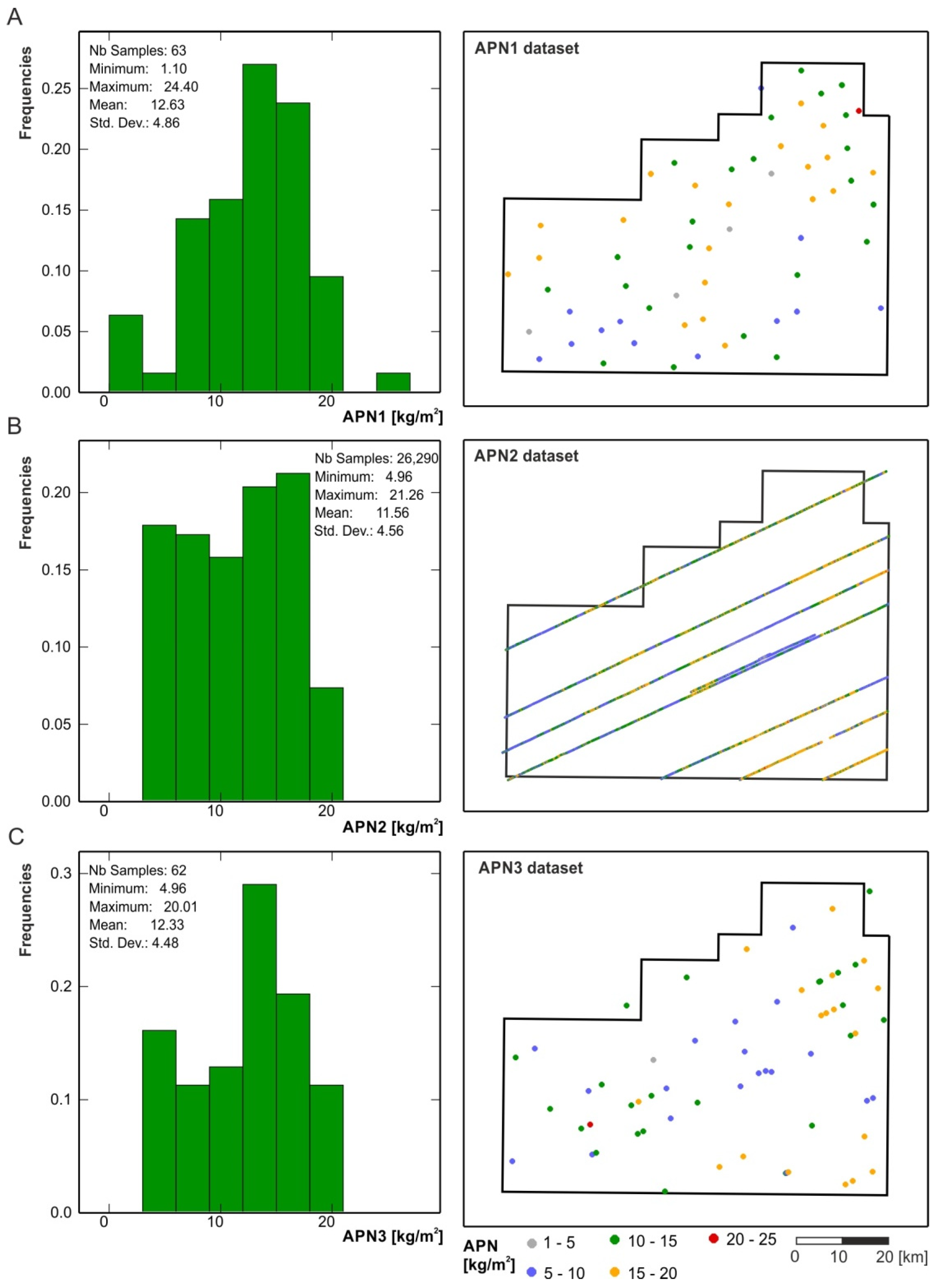
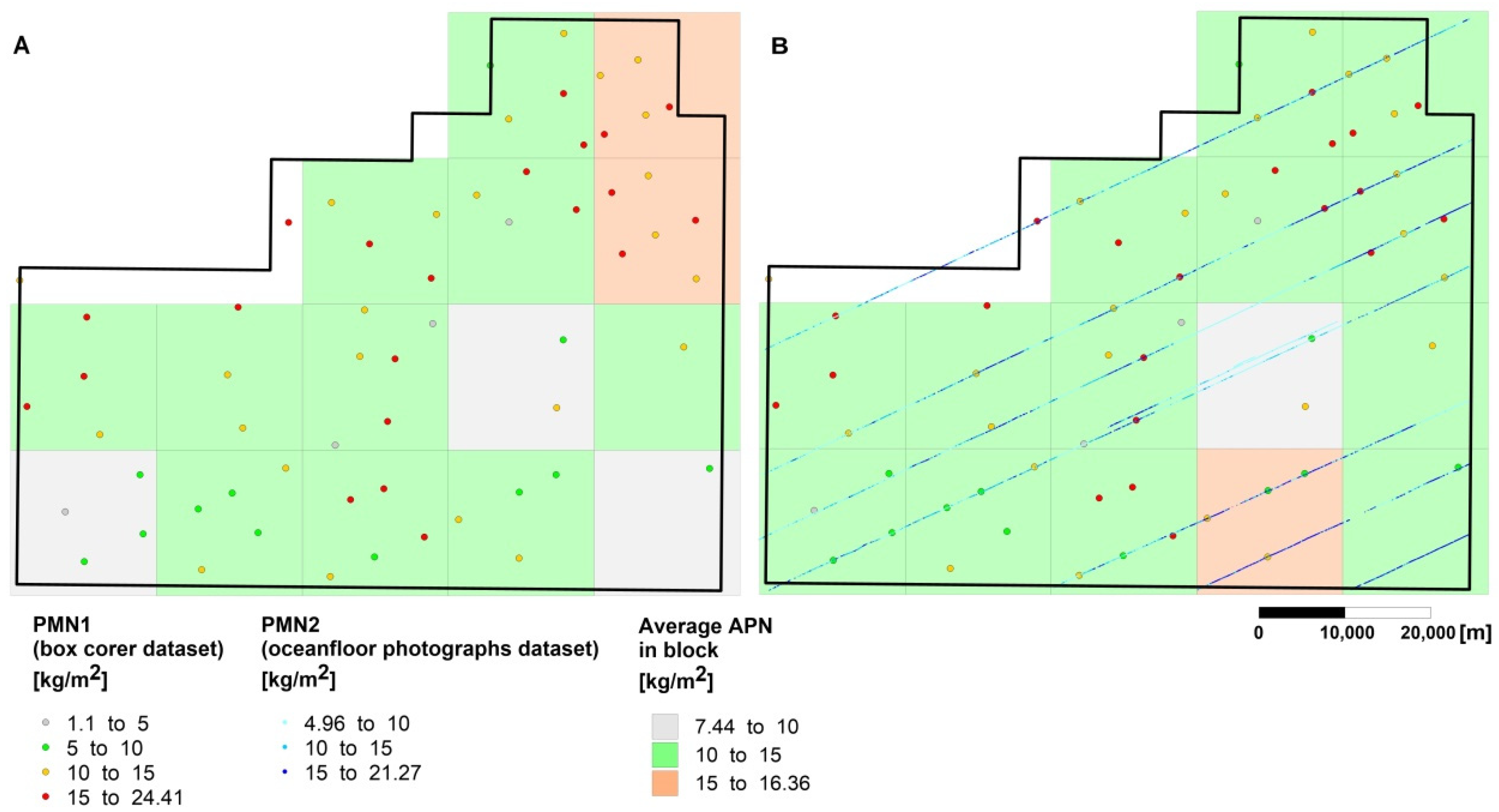
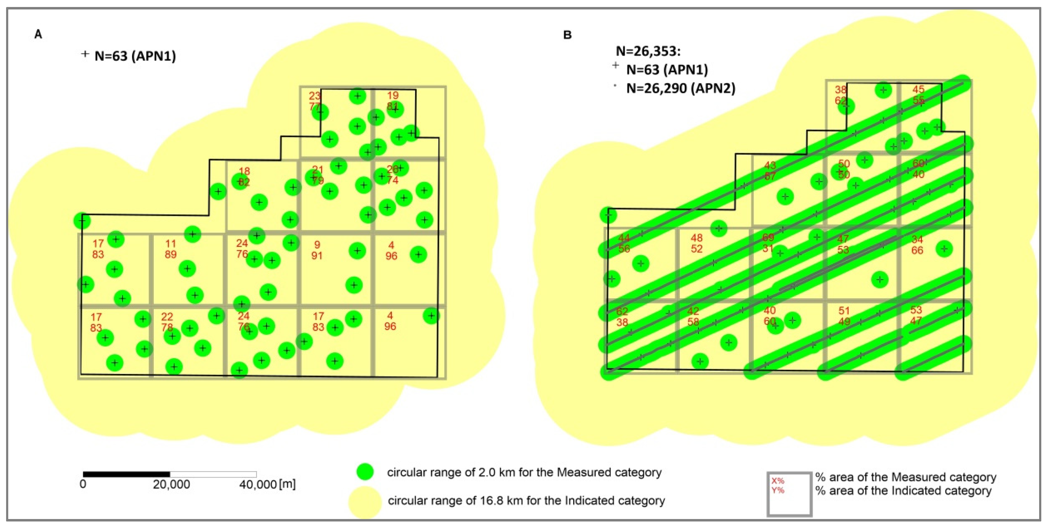
- 63 direct assessments of nodule abundance using the box corers (hereinafter abbreviated as APN1),
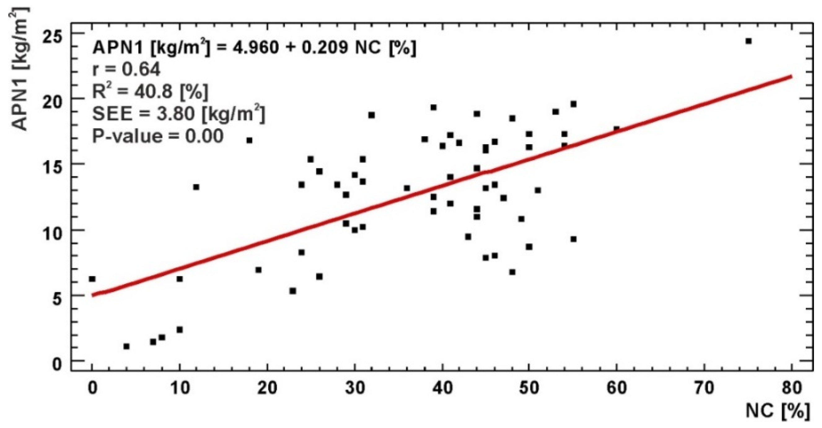
- 63 photographs covering an area of approximately 1.5 m2 each, carried on at the box corer sampling sites, and used to model the relationship between nodule abundance (APN1) and nodule coverage (i.e., the percentage of seafloor covered by the nodules, hereinafter abbreviated NC),
- 26,352 sites of photographic survey of the seafloor (an area of approximately 5 m2), located along the courses of the research vessel using Neptune C-M1 device [19]; on the basis of this photographs PN, the abundance was determined indirectly from regression model and was used to:
- determining the accuracy of PN abundance estimation with ordinary kriging procedure (dataset of 26,290 sites, hereinafter abbreviated APN2),
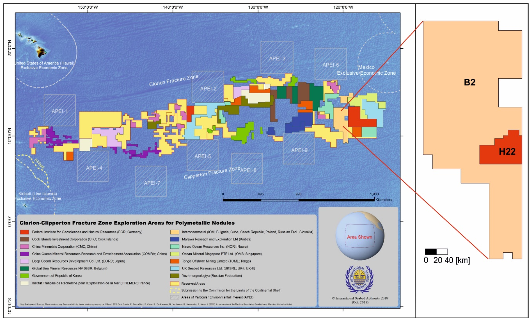
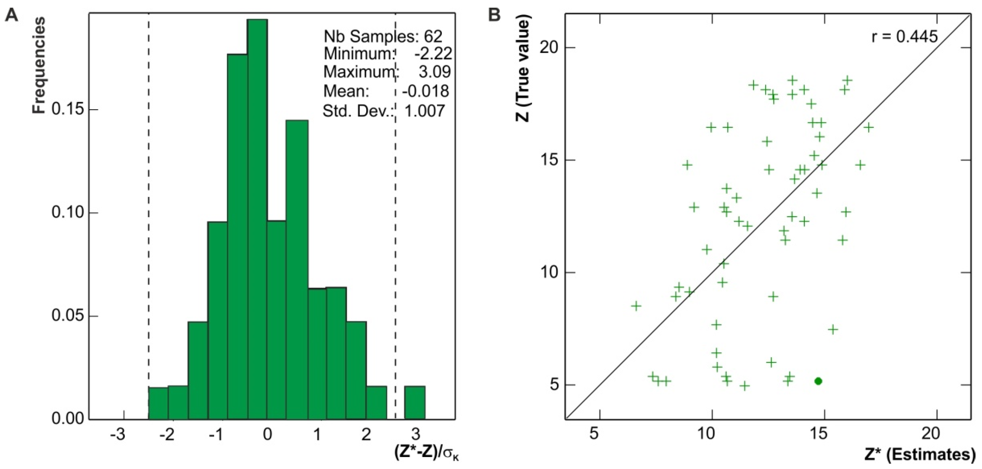
- the cross-validation procedure [23] as the test dataset excluded from the calculations of empirical variograms (dataset of 62 sites randomly selected within the H22 exploration block, hereinafter abbreviated APN3).
4. Methods
- within the entire H22 exploration block of total area about 4200 km2 (i.e., all data collected were included into the kriging procedure),
- within 15 square blocks, each of 17 km × 17 km size and the area of 300 km2, representing roughly the future mining fields selected for annual exploitation, assuming the planned annual production of 3 million metric tons and the average abundance of wet nodules of approximately 10 kg/m2.
5. Results and Discussion
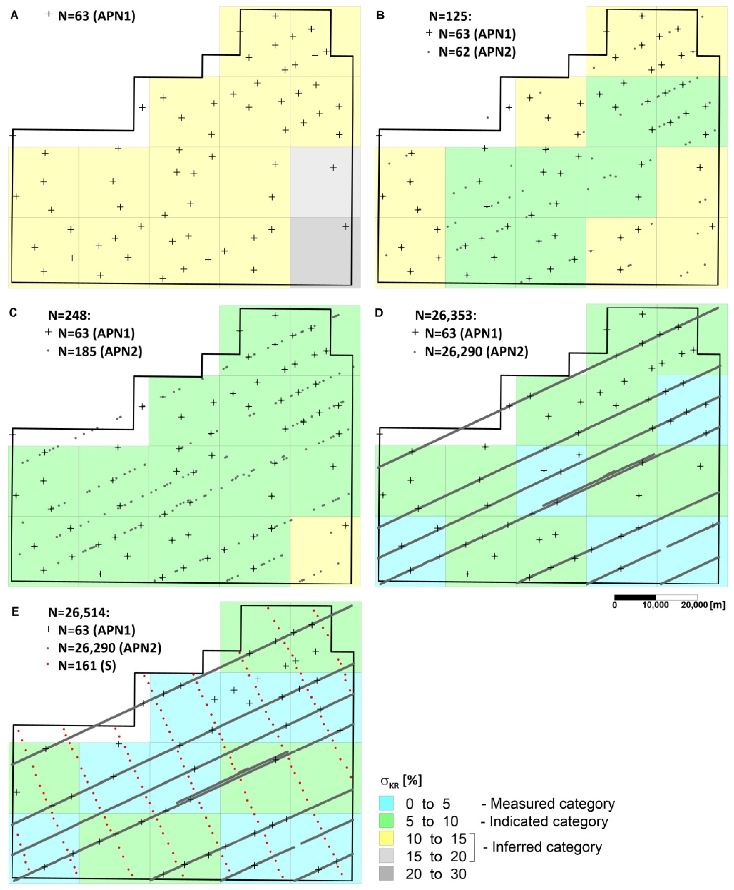
- only the box corer dataset (APN1),
- combined, box corer (APN1) and various size of photographic datasets (APN2),
- full box corer dataset (APN1) and full photographic dataset (APN2) combined with data from sampling sites simulated (S) along the lines perpendicular to the courses of the research vessel.
6. Resource Classification
7. Conclusions
- Achieving a high accuracy of estimation of polymetallic nodule abundance in the IOM area (CCZ, Pacific Ocean) in blocks planned for annual exploitation is difficult and requires a radical increase of density of currently applied sampling grid, which is associated with significant costs and labor intensity of the project.
- The usage of even a small number of seafloor photographs in order to determine the seafloor coverage with the PN significantly modifies the variogram model, especially the evaluation of nugget effect, and increases the estimation accuracy of PN resources. However, this accuracy improvement is not as radical as one would expect, given a huge amount of photographic data. This can be explained by extremely unfavorable, preferential distribution of photographic observations, as the seafloor photographs were taken only along the course lines of the research vessel.
- The inclusion of indirect (photographic) measurements to PN resources estimations must be preceded by solution of a number of problems arising when different (box corer and photographic) datasets are integrated. These include, among others:
- determining the accuracy of automatic computerized contouring of nodules in photographs, which affects the accuracy assessment of PN coverage of the seafloor,
- evaluation of errors that are related to determination of nodule abundance from a regression model linking it to the degree of seafloor nodule coverage,
- examining the local variability of PN coverage of seafloor on the basis of fragments of photographs covering an area of approximately 0.25 m2, corresponding to the area of the box corer horizontal cross-section.
- The classification of PN resources related to the requirements contained in the ISA classification standards should be based on two criteria:
- permissible relative errors of nodule resources estimation (or average abundances) for the whole studied deposit or for its fragments,
- evaluation of the continuity degree of changes in nodules abundance.
- 5.
- In order to achieve both the consistency and the comparability of PN resources classification carried on by various persons for various deposits, reconciliation and standardization of assessment criteria is necessary by all centers involved in estimation of nodule resources. Particularly important is the standardization of: (i) values of permissible errors of PN resource estimations for Measured, Indicated, and Inferred categories, (ii) confidence levels applied to statistical or geostatistical estimations of errors, and (iii) methodology of determination of continuity range of PN abundances.
- 6.
- Due to the fact that the exploration of oceanic deposits is much more difficult in relation to the onshore ones (i.e., significant depths of ocean basins, vast extent of deposit areas, high exploration costs), the classification criteria can be somewhat less strict than proposed in this paper.
- 7.
- The methodology for classifying nodule resources in the Pacific described in the article is a preliminary proposal and should be the material for further discussions and studies.
Author Contributions
Funding
Acknowledgments
Conflicts of Interest
References
- Felix, D. Some Problems in Making Nodule Abundance Estimates from Seafloor Photographs. Mar. Min. 1980, 2, 293–302. [Google Scholar]
- Handa, K.; Tsurusaki, K. Manganese Nodules: Relationship between Coverage and Abundance in the Northern Part of Central Pacific Basin. Geol. Surv. Jpn. 1981, 15, 184–217. [Google Scholar]
- Sharma, R. Quantitative Estimation of Seafloor Features from Photographs and Their Application to Nodule Mining. Mar. Georesources Geotechnol. 1993, 11, 311–331. [Google Scholar] [CrossRef]
- Parianos, J. UPDATED NI 43-101 TECHNICAL REPORT Clarion-Clipperton Zone Project, Pacific Ocean; 127631013-003-R-Rev1; Tonga Offshore Mining Limited, 2013. Available online: http://www.nautilusminerals.com (accessed on 21 January 2020).
- Yoo, C.M.; Joo, J.; Lee, S.H.; Ko, Y.; Chi, S.-B.; Kim, H.J.; Seo, I.; Hyeong, K. Resource Assessment of Polymetallic Nodules Using Acoustic Backscatter Intensity Data from the Korean Exploration Area, Northeastern Equatorial Pacific. Ocean Sci. J. 2018, 53, 381–394. [Google Scholar] [CrossRef]
- Sharma, R.; Khadge, N.H.; Jai Sankar, S. Assessing the Distribution and Abundance of Seabed Minerals from Seafloor Photographic Data in the Central Indian Ocean Basin. Int. J. Remote Sens. 2013, 34, 1691–1706. [Google Scholar] [CrossRef]
- Tsune, A. Effects of Size Distribution of Deep-Sea Polymetallic Nodules on the Estimation of Abundance Obtained from Seafloor Photographs Using Conventional Formulae. In Proceedings of the Eleventh Ocean Mining and Gas Hydrates Symposium; International Society of Offshore and Polar Engineers, Kona, HI, USA, 21–27 June 2015; p. 7. [Google Scholar]
- Park, C.-Y.; Park, S.-H.; Kim, C.-W.; Kang, J.-K.; Kim, K.-H. An Image Analysis Technique for Exploration of Manganese Nodules. Mar. Georesources Geotechnol. 1999, 17, 371–386. [Google Scholar] [CrossRef]
- Sharma, R.; Sankar, S.J.; Samanta, S.; Sardar, A.A.; Gracious, D. Image Analysis of Seafloor Photographs for Estimation of Deep-Sea Minerals. Geo Mar. Lett. 2010, 30, 617–626. [Google Scholar] [CrossRef]
- Park, S.H.; Kim, D.H.; Kim, C.-W.; Park, C.Y.; Kang, J.K. Estimation of Coverage and Size Distribution of Manganese Nodules Based On Image Processing Techniques. In Proceedings of the Second ISOPE Ocean Mining Symposium; International Society of Offshore and Polar Engineers, Seoul, Korea, 24–26 November 1997; pp. 40–44. [Google Scholar]
- Schoening, T.; Kuhn, T.; Jones, D.O.B.; Simon-Lledo, E.; Nattkemper, T.W. Fully Automated Image Segmentation for Benthic Resource Assessment of Poly-Metallic Nodules. Methods Oceanogr. 2016, 15, 78–89. [Google Scholar] [CrossRef]
- Schoening, T.; Jones, D.O.B.; Greinert, J. Compact-Morphology-Based Poly-Metallic Nodule Delineation. Sci. Rep. 2017, 7, 13338. [Google Scholar] [CrossRef] [PubMed]
- Gazis, I.-Z.; Schoening, T.; Alevizos, E.; Greinert, J. Quantitative Mapping and Predictive Modeling of Mn Nodules’ Distribution from Hydroacoustic and Optical AUV Data Linked by Random Forests Machine Learning. Biogeosciences 2018, 15, 7347–7377. [Google Scholar] [CrossRef]
- Peukert, A.; Schoening, T.; Alevizos, E.; Köser, K.; Kwasnitschka, T.; Greinert, J. Understanding Mn-Nodule Distribution and Evaluation of Related Deep-Sea Mining Impacts Using AUV-Based Hydroacoustic and Optical Data. Biogeosciences 2018, 15, 2525–2549. [Google Scholar] [CrossRef]
- Kotlinski, R.A.; Mucha, J.; Wasilewska, M. Deposits of polymetallic nodules in the Pacific: Problems of their reserve estimation. Gospod. Surowcami Miner. Miner. Resour. Manag. 2008, 24, 257–266. [Google Scholar]
- Kotlinski, R.A. Activities of the Interoceanmetal Joint Organization (IOM) in Relation to Deep Seabed Mineral Resources Development. In Proceedings of the Seabed: The New Frontier, ISA, Madrid, Spain, 24–26 February 2010; p. 29. [Google Scholar]
- Abramowski, T.; Stoyanova, V. Deep-Sea Polymetallic Nodules: Renewed Interest as Resources for Environmentally Sustainable Development. In Proceedings of the SGEM2012 Conference Proceedings, Albena, Bulgaria, 17–23 June 2012; Volume 1, pp. 515–522. [Google Scholar]
- Mucha, J.; Wasilewska-Blaszczyk, M.; Kotlinski, R.A.; Maciąg, L. Variability and Accuracy of Polymetallic Nodules Abundance Estimations in the IOM Area—Statistical and Geostatistical Approach. In Proceedings of the Tenth ISOPE Ocean Mining and Gas Hydrates Symposium; International Society of Offshore and Polar Engineers, Szczecin, Poland, 22–26 September 2013; pp. 27–31. [Google Scholar]
- Dreiseitl, I. Deep Sea Exploration for Metal Reserves—Objectives, Methods and Look into the Future. In Deep See Mining Value Chain: Organization, Technology and Development; Abramowski, T., Ed.; Interoceanmetal Join Organization: Szczecin, Poland, 2016; pp. 105–117. [Google Scholar]
- Technical Report on the Interoceanmetal Joint Organization Polymetallic Nodules Project in the Pacific Ocean Clarion-Clipperton Fracture Zone; Part 1; Polish Geological Institute—National Research Institute: Warsaw, Poland, 2016; p. 147.
- ISA. Reporting Standard of the International Seabed Authority for Mineral Exploration Results Assessments, Mineral Resources and Mineral Reserves. 2015. Available online: http:// www.isa.org.jm (accessed on 21 January 2020).
- Clarion-Clipperton Fracture Zone Exploration Areas for Polymetallic Nodules. Available online: https://www.isa.org.jm/contractors/exploration-areas (accessed on 20 January 2020).
- Clark, I. The Art of Cross Validation in Geostatistical Applications. In Proceedings of the 19th Application of Computers and Operations Research in the Mineral Industry; Society of Mining Engineers, Littleton, CO, USA, 14–16 April 1986; pp. 211–220. [Google Scholar]
- STATGRAPHICS Centurion XVII; Statpoint Technologies Inc.: Warrenton, VA, USA, 2014.
- Matheron, G. Traité de Géostatistique Appliquée; Editions Technip: Paris, France, 1962. [Google Scholar]
- Journel, A.G.; Huijbregts, C.J. Mining Geostatistics; Academic Press: London, UK, 1979; p. 600. [Google Scholar]
- Deutsch, C.V.; Journel, A.G. GSLIB Geostatistical Software Library and User’s Guide; Oxford University Press: New York, NY, USA, 1992; p. 340. [Google Scholar]
- Isaaks, E.H.; Srivastava, R.M. An Introduction to Applied Geostatistics; Oxford University Press: New York, NY, USA, 1989; p. 561. [Google Scholar]
- Goovaerts, P. Geostatistics for Natural Resources Evaluation; Oxford University Press: New York, NY, USA, 1997; p. 483. [Google Scholar]
- Armstrong, M. Basic Linear Geostatistics, 1st ed.; Springer: Berlin/Heidelberg, Germany, 1998; p. 155. [Google Scholar]
- Clark, I.; Harper, W.V. Practical Geostatistics 2000; Geostokos (Ecosse) Limited: Scotland, UK, 2008; p. 430. [Google Scholar]
- Chautru, J.M.; Morel, Y.; Herrouin, G. Geostatistical Simulation of a Commercial Polymetallic Nodule Mining Site. In Proceedings of the Twentieth International Symposium on the Application of Computers and Mathematics in the Mineral Industries, Johannesburg, South Africa, 19–23 October 1987; Volume 3, pp. 177–185. [Google Scholar]
- A Geological Model of Polymetallic Nodule Deposits in the Clarion-Clipperton Fracture Zone. Available online: http:// www.isa.org.jm (accessed on 21 January 2020).
- Mucha, J.; Wasilewska-Blaszczyk, M.; Dudek, M. The Accuracy of Polymetallic Nodule Resources Estimation in the Pacific in the Interoceanmetal Area Based on Samples Collected Using a Box Corer. In Proceedings of the 19th International Multidisciplinary Scientific GeoConference SGEM 2019, Albena, Bulgaria, 30 June–6 July 2019. [Google Scholar]
- Kalyan, B.; Ganesan, V.; Chitre, M.; Vishnu, H. Optimal Point Planning for Abundance Estimation of Polymetallic Nodules. In OCEANS 2017—Anchorage; IEEE: Anchorage, AK, USA, 2017; pp. 1–6. [Google Scholar]
- Knobloch, A.; Kuhn, T.; Rühlemann, C.; Hertwig, T.; Zeissler, K.-O.; Noack, S. Predictive Mapping of the Nodule Abundance and Mineral Resource Estimation in the Clarion-Clipperton Zone Using Artificial Neural Networks and Classical Geostatistical Methods. In Deep-Sea Mining: Resource Potential, Technical and Environmental Considerations; Sharma, R., Ed.; Springer: Cham, The Netherlands, 2017; pp. 189–212. [Google Scholar]
- Singh, T.R.P.; Sudhakar, M. Statistical Properties of Distribution of Manganese Nodules in Indian and Pacific Oceans and Their Applications in Assessing Commonality Levels and in Exploration Planning. In Deep-Sea Mining: Resource Potential, Technical and Environmental Considerations; Sharma, R., Ed.; Springer: Cham, The Netherlands, 2017; pp. 213–228. [Google Scholar]
- CRIRSCO. International Reporting Template for the Public Reporting of Exploration Results, Mineral Resources and Mineral Reserves; International Council on Mining & Metals (ICMM), 2013. Available online: http://www.crirsco.com (accessed on 21 January 2020).
- CRIRSCO. International Reporting Template for the Public Reporting of Exploration Results, Mineral Resources and Mineral Reserves; International Council on Mining & Metals (ICMM), 2019. Available online: http://www.crirsco.com (accessed on 21 January 2020).
- Larkin, B.J. Geostatistical Study Zuun Mod Molybdenum Deposit Mongolia; GeoCheck Pty. Ltd.: Queensland, Austrila, 2008; p. 56. [Google Scholar]
- Mucha, J.; Wasilewska-Blaszczyk, M.; Auguscik, J. Categorization of Mineral Resources Based upon Geostatistical Estimation of the Continuity of Changes of Resource Parameters. In Proceedings of the 17th Annual Conference of the International Association for Mathematical Geosciences, Freiberg, Germany, 5–13 September 2015. [Google Scholar]
- Mucha, J.; Wasilewska-Blaszczyk, M. Geostatistical Support for Categorization of Metal Ore Resources in Poland. Gospod. Surowcami Miner. Miner. Resour. Manag. 2015, 31, 21–34. [Google Scholar] [CrossRef]


| Variogram Type | Source of Data | Variogram Model | C0 | Ci | ai [m] | |
|---|---|---|---|---|---|---|
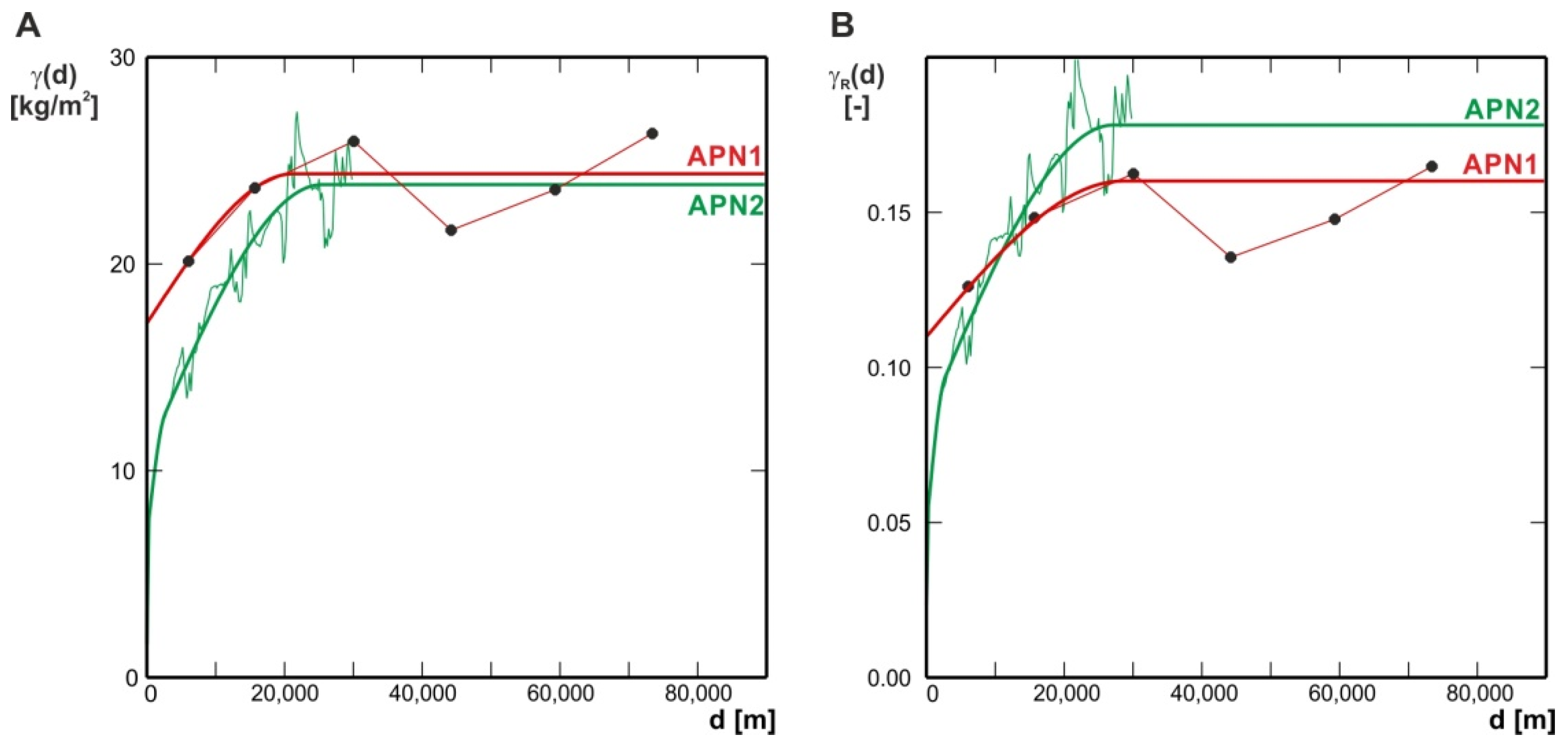
| Classical (γ) | Box corer dataset (APN1) N = 63 | Simple spherical | 17.13 | 70.3 | C1 = 7.23 | a1 = 21,302 |
| Classical (γ) | Seafloor photographs dataset (APN2) N = 26,290 | Nested spherical | 1.59 | 6.7 | C1 = 5.21 C2 = 13.11 C3 = 3.92 | a1 = 323 a2 = 25,465 a3 = 2678 |
| C = C1 + C2 + C3 = 22.24 | ||||||
| Relative (γR) | Box corer dataset (APN1) N = 63 | Simple spherical | 0.110 | 68.8 | C1 = 0.050 | a1 = 28,546 |
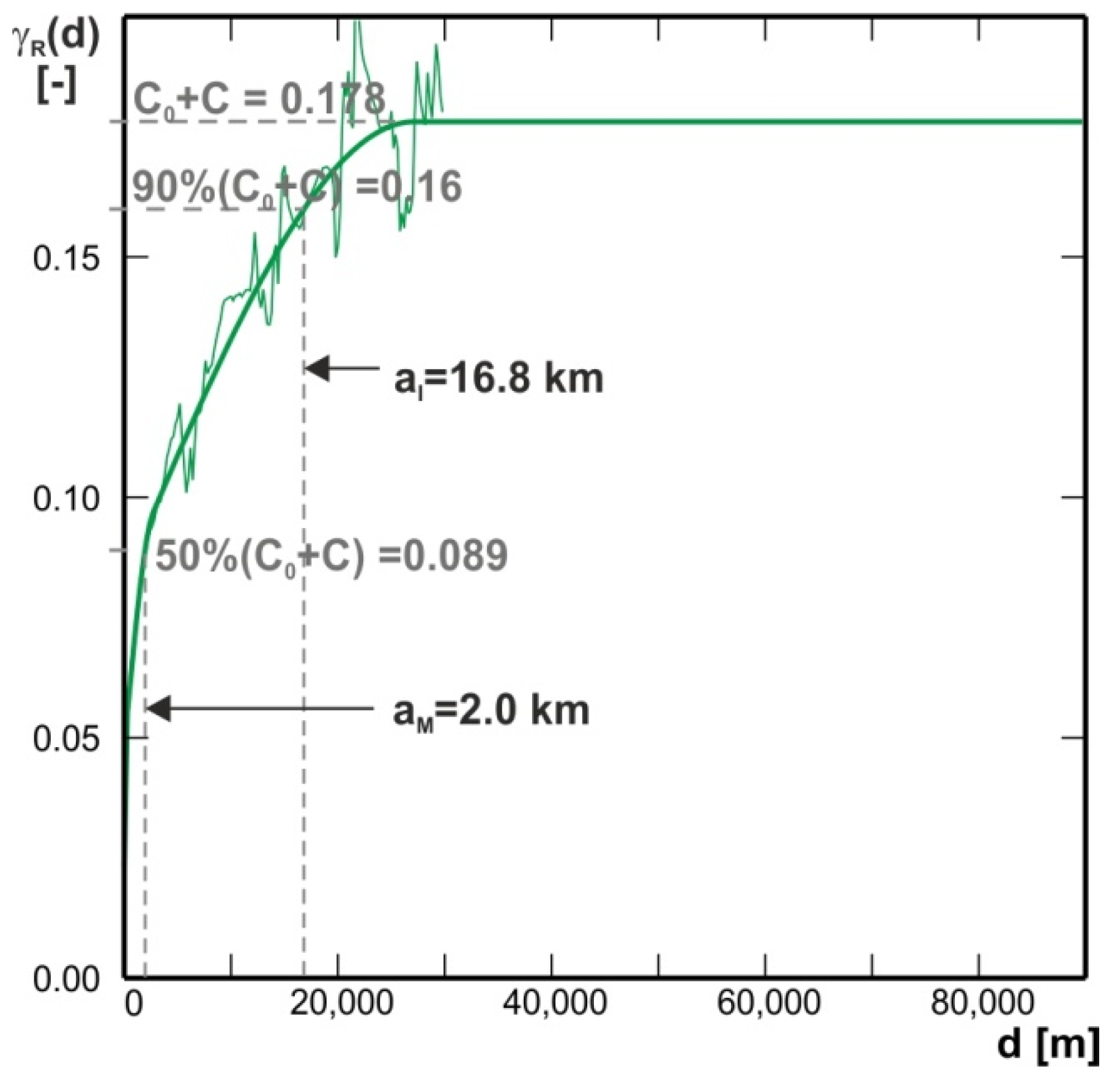
| Relative (γR) | Seafloor photographs dataset (APN2) N = 26,290 | Nested spherical | 0.023 | 12.9 | C1 = 0.025 C2 = 0.095 C3 = 0.035 | a1 = 206 a2 = 27,196 a3 = 2718 |
| C = C1 + C2 + C3 = 0.155 |
| Number of Data Used for Estimation | Relative Kriging Standard Errors σKR [%] | |||||
|---|---|---|---|---|---|---|
| APN1 | APN2 | Simulated Sampling Sites (S) | Total | Minimum | Maximum | Median |
| 63 | 63 | 10.6 | 26.9 | 13.0 | ||
| 63 | 62 | 125 | 7.4 | 11.6 | 10.1 | |
| 63 | 124 | 187 | 6.5 | 10.7 | 8.7 | |
| 63 | 185 | 248 | 6.0 | 10.1 | 8.2 | |
| 63 | 26,290 | 26,353 | 3.7 | 8.3 | 6.3 | |
| 63 | 26,290 | 56 | 26,409 | 3.5 | 7.9 | 5.5 |
| 63 | 26,290 | 161 | 26,514 | 3.4 | 7.1 | 5.0 |
| Number of Data | Number of Blocks | |||||
|---|---|---|---|---|---|---|
| Accuracy of PN Resources Estimation | Continuity of PN Abundance | |||||
| Measured | Indicated | Inferred | Measured | Indicated | Inferred | |
| 63 | 0 | 0 | 15 | 0 | 15 | - |
| 125 | 0 | 7 | 8 | - | - | - |
| 248 | 0 | 14 | 1 | - | - | - |
| 26,353 | 5 | 10 | 0 | 5 | 10 | - |
| 26,514 | 8 | 7 | 0 | - | - | - |
© 2020 by the authors. Licensee MDPI, Basel, Switzerland. This article is an open access article distributed under the terms and conditions of the Creative Commons Attribution (CC BY) license (http://creativecommons.org/licenses/by/4.0/).
Share and Cite
Mucha, J.; Wasilewska-Błaszczyk, M. Estimation Accuracy and Classification of Polymetallic Nodule Resources Based on Classical Sampling Supported by Seafloor Photography (Pacific Ocean, Clarion-Clipperton Fracture Zone, IOM Area). Minerals 2020, 10, 263. https://doi.org/10.3390/min10030263
Mucha J, Wasilewska-Błaszczyk M. Estimation Accuracy and Classification of Polymetallic Nodule Resources Based on Classical Sampling Supported by Seafloor Photography (Pacific Ocean, Clarion-Clipperton Fracture Zone, IOM Area). Minerals. 2020; 10(3):263. https://doi.org/10.3390/min10030263
Chicago/Turabian StyleMucha, Jacek, and Monika Wasilewska-Błaszczyk. 2020. "Estimation Accuracy and Classification of Polymetallic Nodule Resources Based on Classical Sampling Supported by Seafloor Photography (Pacific Ocean, Clarion-Clipperton Fracture Zone, IOM Area)" Minerals 10, no. 3: 263. https://doi.org/10.3390/min10030263
APA StyleMucha, J., & Wasilewska-Błaszczyk, M. (2020). Estimation Accuracy and Classification of Polymetallic Nodule Resources Based on Classical Sampling Supported by Seafloor Photography (Pacific Ocean, Clarion-Clipperton Fracture Zone, IOM Area). Minerals, 10(3), 263. https://doi.org/10.3390/min10030263