Abstract
The Fe(II) monosulfide mineral mackinawite (FeS) is an important phase in low-temperature iron and sulfur cycles, yet it is challenging to characterize since it often occurs in X-ray amorphous or nanoparticulate forms and is extremely sensitive to oxidation. Moreover, the electronic configuration of iron in mackinawite is still under debate. Mössbauer spectroscopy has the potential to distinguish mackinawite from other FeS phases and provide clarity on the electronic configuration, but conflicting results have been reported. We therefore conducted a Mössbauer study at 5 K of five samples of mackinawite synthesized through different pathways. Samples show two different Mössbauer patterns: a singlet that remains unsplit at all temperatures studied, and a sextet with a hyperfine magnetic field of 27(1) T at 5 K, or both. Our results suggest that the singlet corresponds to stoichiometric mackinawite (FeS), while the sextet corresponds to mackinawite with excess S (FeS1+x). Both phases show center shifts near 0.5 mm/s at 5 K. Coupled with observations from the literature, our data support non-zero magnetic moments on iron atoms in both phases, with strong itinerant spin fluctuations in stoichiometric FeS. Our results provide a clear approach for the identification of mackinawite in both laboratory and natural environments.
1. Introduction
Iron(II) monosulfide, FeS, also known as the mineral mackinawite, is widespread in low-temperature aqueous environments. As a metastable phase, it plays an important part in pyrite formation pathways in soils and sediments, and hence participates in many (bio)geochemical processes (e.g., [1] and references therein). Mackinawite has likely been present on Earth since the Hadean eon [2] and might have played a role in the origin of life [3,4]. Industrially, it has potential for microbial fuel cells [5] and exhibits the magnetic characteristics of isostructural high-temperature Fe-based superconductors [6].
Despite its significance and although it has been studied for several decades, identification and characterization of mackinawite using standard mineralogical tools remain challenging. Mackinawite crystallizes in a tetragonal structure with space group P4/nmm where iron atoms occupy edge-shared tetrahedra that are arranged in layers [7], but amorphous and nanoparticulate forms have also been identified, e.g., [8,9], that generally precede crystallization. Moreover, there are conflicting conclusions regarding the electronic configuration of iron in mackinawite—either high-spin Fe(II), e.g., [1,6], or low-spin Fe(II), e.g., [10,11,12]. 57Fe Mössbauer spectroscopy, e.g., [13,14], probes hyperfine interactions at the iron nucleus and does not require long-range ordering of the crystal structure. It should therefore be well suited to the identification of mackinawite, for example, in natural anoxic sediments, and the elucidation of its electronic configuration. However, Mössbauer spectra reported for mackinawite vary significantly, from a singlet [12,15,16] to a sextet [17] to a singlet–sextet mixture [10] to multiple sextets [18], and therefore this technique has not been used for identification.
Mössbauer data also conflict with calculated results on Fe spin states and the closely related magnetic properties of mackinawite. Rickard and Luther [1] assign Fe to be high spin (HS) in mackinawite, whereas Vaughan and Ridout [12] and Mullet and coauthors [10] designate it as low spin (LS) based on Mössbauer observations. Density functional theory (DFT) calculations have also led to opposing conclusions with regard to the magnetic moment of Fe in mackinawite. While Devey and coauthors [19] calculated a non-magnetic stable ground state, iron should have a substantial magnetic moment according to Subedi and coauthors [20]. Unpaired electrons are necessary for a magnetic moment to arise, and consideration of the accompanying spin is challenging with DFT [21]. Mössbauer spectroscopy should be able to provide clarity, yet reported Mössbauer results are similarly confusing. They show the absence of magnetic ordering even when samples are cooled down to below 4.2 K [12,15] but also magnetic ordering already at room temperature [18], while Mullet and coauthors [10] observed a mix of phases in spectra obtained at ~11 K with some showing magnetic ordering and others not.
In this study, we produced mackinawite through different formation pathways and characterized run products using Mössbauer spectroscopy. The results allow us to (i) identify the Mössbauer spectral pattern associated with mackinawite; (ii) explain differences in spectral patterns according to the formation pathways; and (iii) elucidate the electronic configuration of iron in mackinawite based on our results and those in the literature.
2. Materials and Methods
2.1. Sample Synthesis
All sample synthesis and preparation took place in an anoxic glove box system with a working atmosphere of N2 (99.99%) (Unilab Glovebox, M. Braun, and Jacomex Glovebox, Jacomex) because of the sensitivity of mackinawite to oxygen. All solutions were prepared inside the glove box with deionized water (18 MΩ) that had been purged with N2 for 1 h prior to transferring into the glove box. All chemicals were analytical grade.
- Sample S1: filtered FeS precipitate from Fe(II) and S(-II) solutions
Reagent solutions were prepared in crimp bottles sealed with septa and aluminum caps. The pre-weighed chemicals (FeCl2·4H2O and Na2S) were each dissolved in 100 mL deionized and degassed water to obtain a Fe or S concentration of 2 mol·L−1. The Fe(II) solution was then slowly injected into the S(-II) solution with a syringe until a small excess of sulfide of ca. 0.1 mol·L−1 was left. A black precipitate appeared immediately. The solution in the crimp bottle was stirred gently with a Teflon-coated magnetic stirring bar during the entire reaction. After all of the Fe(II) solution had been injected, the precipitate was left in the bottle for at least another 24 h up to a maximum of 1 week. A sample was directly filtered from the suspension (Ø 13 mm, 0.45 µm, cellulose filter paper) and measured immediately.
- Sample S2: freeze-dried FeS
A second sample was prepared following the procedure for sample S1. The black precipitate was collected via centrifuging, decanting the supernatant, washing with deionized water, and centrifuging again. The final product was freeze-dried, stored in the sealed crimp vial under N2 atmosphere, and measured after one month of storage.
- Sample S3a: FeS from interaction between Fe(III) and S(-II) with low Fe/S ratio
Preparation followed the experimental setup already described [17,22]. Briefly, 450 mL S(-II) solution (approximately 8 mmol·L−1 Na2S solution) was adjusted to pH 7.0 by adding HCl (c = 1 mol·L−1) in a closed reaction vessel. Subsequently, 50 mL of suspension containing a preselected amount of synthetic lepidocrocite was added. The pH was kept constant at pH = 7.00 ± 0.05 with HCl (c = 0.1 mol·L−1) using a pH-Stat device (Titrino, Metrohm). The suspension was gently stirred with a Teflon-coated magnetic stirring bar during the entire experiment. The initial molar ratio of Fe/S was adjusted to be “low” (Fe/S = 0.5) in order to obtain excess S(-II). The sample was taken by filtration (Ø 13 mm, 0.45 µm, cellulose filter paper) after 72 h and measured immediately.
- Sample S3b: FeS from interaction between Fe(III) and S(-II) with high Fe/S ratio
A second sample was prepared following the procedure for sample S3a, except with an initial “high” Fe/S molar ratio (Fe/S = 2.8) in order to obtain excess lepidocrocite after complete S(-II) consumption. The sample was taken by filtration (Ø 13 mm, 0.45 µm, cellulose filter paper) after 3 h and measured immediately.
- Sample 4: FeS from pure polysulfide solution
A polysulfide solution was prepared and equilibrated for 4 h after adding elemental sulfur to a sulfide (0.1 M) solution obtained by dissolving Na2S in deionized water. The solution turned from colorless to vivid yellow. Not all of the elemental sulfur was completely dissolved, but the concentration of polysulfide was not measured. FeCl2 solution (0.1 M) was then added dropwise into the filtered, vividly yellow polysulfide solution while the solution was slowly shaken. The polysulfide solution was slightly in excess to FeCl2. A black precipitate formed immediately. After 5 days, 20 mL of the suspension was collected and centrifuged. The supernatant was decanted, and the black residue was dried under N2 flow in an airtight container outside the glove box.
- Sample 5: lepidocrocite (γ-FeOOH)
Synthetic lepidocrocite was prepared after Schwertmann and Cornell [23] as previously described in detail [22].
2.2. Mössbauer Spectroscopy
Filters with the solid fraction on top or freeze-dried powders were sealed between two layers of Kapton tape inside the glove box after small amounts of excess liquid had been carefully removed. The samples were placed in a sealed bottle to avoid contact with air during transportation from the glove box to the Mössbauer spectrometer and were measured immediately. The sample chamber of the Mössbauer spectrometer was pre-cooled to ~5 K and flushed with helium gas upon opening. The sample was frozen immediately upon insertion into the cryostat, and the sample chamber was sealed to be airtight and pumped to remove any air that might have entered the chamber. Mössbauer spectra were collected with a WissEl or a SeeCo Mössbauer transmission spectrometer, using a 57Co in Rh matrix γ-ray source mounted on a constant acceleration drive system. Samples were cooled in either a Janis closed-cycle helium gas cryostat or a Janis continuous flow cryostat and measured at ~5 K. During measurement, the samples were kept in vacuum or in a low-pressure helium atmosphere to avoid oxidation. The velocity scales were calibrated using α-Fe foil at room temperature. Spectral fitting was carried out using Recoil software (University of Ottawa, Ottawa, ON, Canada).
2.3. X-Ray Diffraction (XRD)
A second synthesis of sample S1 was performed using the same procedure described above. The sample was directly filtered from the suspension (Ø 13 mm, 0.45 µm, cellulose filter paper) and allowed to dry within the glovebox overnight for 12 h. Powder X-ray diffraction (XRD) patterns were collected at the University of Edinburgh using a Bruker D8 Advance with a Sol-X Energy Dispersive detector (Bruker, Billerica, MA, USA) with the sample contained in an X-ray transparent controlled atmosphere holder. XRD patterns were collected using Cu Kα radiation without a monochromator using scans between 10° and 70° 2θ. Mineral phases were identified using the International Center for Diffraction Data (ICDD) Powder Diffraction File 2 (PDF-2) database and DIFFRACplus EVA v.2 software from Bruker.
3. Results
Mössbauer spectra of sample S1 collected at 293 and 5 K show a singlet (Figure 1) with hyperfine parameters given in Table 1. The XRD pattern (Figure 2) confirms mackinawite. A singlet also appears with a similar center shift in the spectrum from sample S2 (Figure 3), but it is broader and accompanied by a magnetic subspectrum that resembles the magnetic spectrum from samples 3a and 4. The magnetic spectrum is broad and asymmetric, but nevertheless has the appearance of a sextet. We fit the data using Voigt-based fitting (VBF) analysis which considers the broadening to arise from Gaussian distributions of hyperfine parameters [24]. Correlations between hyperfine parameters lead to asymmetric broadening, which is treated in the VBF model by a linear coupling parameter. We obtained good fits to the broadened sextets using a single Gaussian component in the VBF model, with fit parameters given in Table 1. The similarity between all average hyperfine parameter values (center shift <CS>, quadrupole shift <ε>, and magnetic hyperfine field <B>) for all three sextets in Figure 3 strongly suggests that they are associated with the same phase. Similar to the singlet, variations in sextet linewidth are likely due to slight variations in next-nearest neighbor environments. The average hyperfine magnetic field of this VBF sextet is 27(1) T at 5 K, so we will refer to it as the 27 T phase.
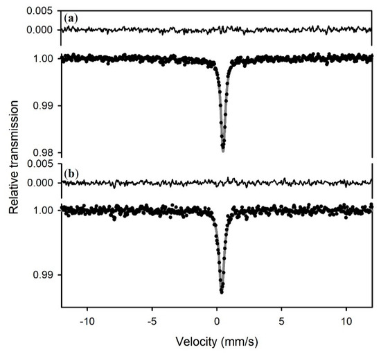
Figure 1.
Mössbauer spectra of sample S1 collected at (a) room temperature (293 K); and (b) 5 K. Spectra were fit to a singlet with parameters given in Table 1. The fitted curve is shown in gray and the residuals (difference between experimental data and calculated curve) are shown above the spectra.

Table 1.
Hyperfine parameters derived from fits to Mössbauer spectra.
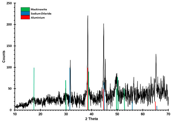
Figure 2.
XRD pattern of sample S1. Green vertical lines indicate those peaks resulting from mackinawite. Sodium chloride (blue vertical lines) is unwashed salt resulting from sample preparation and drying of the sample. Aluminum reflections (red vertical lines) stem from the sample holder. The spectrum is noisy because of Fe fluorescence and poor long-range ordering resulting from the small size of the crystals. Results demonstrate the need for other identification techniques such as Mössbauer spectroscopy.
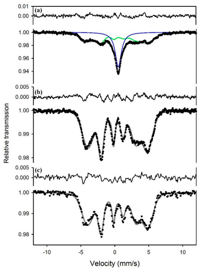
Figure 3.
Mössbauer spectra at 5 K of (a) sample S2, (b) sample S3a, and (c) sample S4. The upper spectrum was fit to a singlet (blue) and a Voigt-based fitting (VBF) sextet (green), while the middle and lower spectra were each fit to one VBF sextet. All three sextets have similar average hyperfine parameters that are given in Table 1.
The spectrum of pure lepidocrocite (sample S5) is a magnetic spectrum (Figure 4, bottom) that can be fit to one VBF sextet with a magnetic hyperfine field of 44 T at 5 K (Table 1). The same 44 T sextet appears in the spectrum of sample S3b, accompanied by a VBF sextet corresponding to the 27 T phase (Figure 4, top).
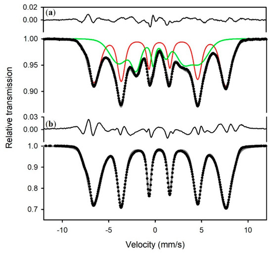
Figure 4.
Mössbauer spectra at 5 K of (a) sample S3b, and (b) sample S5. The upper spectrum was fit to a VBF sextet (green) assigned to the 27 T phase and a VBF sextet (red) assigned to lepidocrocite, while the lower spectrum was fit to one VBF sextet assigned to lepidocrocite. Hyperfine parameters are given in Table 1.
To investigate the 27 T phase further, we collected Mössbauer spectra of sample S3a at different temperatures (Figure 5). The spectrum at 77 K is magnetic and can be fit to one VBF sextet with two Gaussian hyperfine magnetic field distribution components (Figure 5, inset), while the spectrum at 140 K is paramagnetic. We fit the paramagnetic spectrum to one VBF quadrupole doublet, where the asymmetry is accounted for by a correlation between the center shift and quadrupole splitting (Table 1).
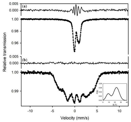
Figure 5.
Mössbauer spectra of sample 3a at (a) 140 K, and (b) 77 K. The lower spectrum was fit to one VBF sextet with two Gaussian distributions of hyperfine magnetic fields (inset), while the upper spectrum was fit to one VBF doublet with one Gaussian distribution of quadrupole splitting. The bimodal distribution of hyperfine magnetic fields at 140 K may indicate variations in magnetic exchange between sites. Hyperfine parameters are given in Table 1.
4. Discussion
4.1. Different Spectral Patterns and Implications for Structure and Transformation Processes
Our results suggest that both the singlet and the sextet (27 T phase) represent FeS identified as mackinawite by other methods. The wet-filtered material (sample S1) was synthesized following a protocol commonly used for FeS synthesis, e.g., [25], and Hellige and coauthors [26] and Peiffer and coauthors [27] identified mackinawite on the basis of 5 Å d-spacings observed with transmission electron microscopy (TEM) in experiments sulfidizing lepidocrocite that were identical to ours. Both spectral patterns have been reported in the literature in connection with mackinawite. The single line is most commonly observed, e.g., [10,12,15], while the six-line pattern with a 27 T magnetic field has also been observed [17]. The 27 T phase occurs in three of our samples that were derived from different starting conditions and is therefore a reproducible spectral pattern.
How can two different spectral patterns arise for a single mineral? It is important to note that the literature describing mackinawite refers to different forms of this mineral. Mackinawite is named after its type location, the Mackinaw Mine (Snohomish county, Washington, DC, USA). Most of the physical properties measured in mackinawite formed in magmatic environments. However, this type of mackinawite tends to contain a significant portion of Ni, e.g., [28,29], and the relatively large crystals are not necessarily representative of the nanoparticulate form found in anoxic sediments. In the laboratory, mackinawite is precipitated as pure stoichiometric FeS from solutions containing dissolved Fe(II) and sulfide. Fe(II) may be added as a salt or by oxidative dissolution of Fe metal. Similarly, sulfide is added either as a salt or by bubbling H2S through the solution. Mackinawite precipitates with particle sizes in the range of 2–10 nm, and grows by particle aggregation [30]. It is an often transient mineral sensitive to oxidation and transforms into more stable iron sulfides, in particular pyrite. The crystal structure of synthetic mackinawite has tetragonal symmetry (P4/nmm), where iron occupies almost perfectly regular FeS4 tetrahedrons [7].
The formation pathways suggest that the single-line subspectrum represents pure mackinawite with a 1:1 FeS stoichiometry, while the 27 T six-line subspectrum represents mackinawite with a different stoichiometry. The single-line subspectrum is remarkable for its lack of quadrupole splitting, which is consistent with a spherically symmetric electron shell such as for an undistorted tetrahedral coordination environment.
This symmetry appears to be broken in the case of the 27 T six-line pattern, which not only reveals a significant quadrupole shift but also magnetic ordering. We will discuss the significance of magnetic ordering further below. Candidates for breaking the symmetry/distorting the coordination environment are O(-II) or polysulfides substituting for S(-II), Fe(III) substituting for Fe(II), Fe deficiency, and/or a restructuring of the crystal lattice as an onset of mineral transformation. Oxygen may come from the air during the freeze-drying process or from the sulfidized iron oxide. Polysulfides may come from excess sulfide in solution reacting with elemental sulfur (generated via sulfide oxidation) or from the reaction of Fe(III) with aqueous sulfide, forming S(0). Small amounts of Fe(III) may have been introduced with Fe(II) salt during synthesis. Fe(III) may also result from oxidation or may be incorporated from the sulfidized iron oxide. Indeed, Fe(III)-S and Fe(II)-O bonds as well as polysulfides have been observed on the surface of freeze-dried mackinawite [10] and in connection with mackinawite formed during sulfidation of iron oxyhydroxides [22].
Incorporation of some Fe(III) would create a mixed-valent sulfide similar to greigite, a mineral characterized by its strong magnetic properties [31]. The Mössbauer parameters of greigite [32,33] are not consistent with those observed here, but White and co-workers [4] suggested an Fe(III)-mackinawite intermediate in the mackinawite–greigite transition. However, there is a line of evidence that indicates that the 27 T six-line subspectrum observed repeatedly by us and reported by Wan and co-workers [17] does not result from Fe(III) incorporation.
The 27 T six-line pattern occurs most prominently in the sulfidation of lepidocrocite at a low Fe/S ratio (0.5) (Figure 3). In this experiment, the excess of sulfide dictates that all Fe is reduced to Fe(II). Wan and co-workers [22] confirmed this in a similar experiment using goethite instead of lepidocrocite, where they observed the presence of polysulfides (S2(-II), Sn(-II)) and elemental sulfur (S8) on mineral surfaces. Since mackinawite crystals grow by particle aggregation [30], incorporation of polysulfides and elemental sulfur would lead to mackinawite with a slight excess in S. A deviation from stoichiometry with less Fe than S has been shown to result in magnetic ordering [34]. A slight excess of sulfide may also explain the occurrence of this six-line pattern upon freeze drying of precipitated mackinawite. We tested this hypothesis by synthesizing mackinawite from a pure polysulfide solution. The resulting Mössbauer spectrum (Figure 3, bottom) shows the same 27 T six-line pattern, and fitting reveals that the hyperfine parameters are essentially the same (Table 1). We therefore assign the 27 T sextet to FeS1+x.
The FeS1+x sextet is broad and asymmetric, indicating a variation in the Fe environment in the crystal lattice. Such a variation would not be expected for pure tetragonal FeS without vacancies or impurities, where all Fe positions would be equal, but is entirely consistent with mackinawite incorporating polysulfides and elemental sulfur. The distribution of quadrupole splitting values that causes asymmetric broadening in the 140 K spectrum is consistent with the distribution of hyperfine magnetic fields in the magnetically ordered phase. However, we cannot entirely rule out quadrupole asymmetry due to relaxation effects as in other magnetically ordered Fe(II) compounds such as siderite [35] or the possibility of multiple iron environments in the paramagnetic phase.
4.2. Electronic Configuration of Iron in Mackinawite
After decades of research, details of the electronic configuration of mackinawite still remain unclear (see Section 1). One of the most puzzling observations from previous Mössbauer measurements [10,12,15] and the present study is the absence of magnetic ordering even at liquid helium temperature. The single-line spectrum that we attributed to pure mackinawite with 1:1 FeS stoichiometry as detailed above is observed over the entire temperature range from room temperature to liquid helium conditions (Figure 1). A particle size effect, i.e., superparamagnetism resulting from particle sizes in the nanometer range, can be excluded. Superparamagnetism can be lifted by cooling mineral samples below their specific Curie or Neél temperatures (TC or TN, respectively) and/or by applying an external magnetic field. Bertaut and co-workers [15] cooled their samples down to 1.7 K and still did not observe magnetic ordering, and Vaughan and Ridout [12] applied an external magnetic field at liquid helium temperature but also failed to observe any magnetic ordering. In addition, the particles in which Mullet and co-workers [10] observed the single-line subspectrum were in the micrometer range.
Magnetic ordering in the mineral structure would lead to splitting of the single line due to the magnetic dipole interaction, for which (1) the nucleus must possess a magnetic dipole moment, and (2) there must be a magnetic field present at the nucleus. Unpaired valence electrons in the electron shell would produce a magnetic field below the magnetic ordering temperature (TC or TN). The Mössbauer parameters constrain the spin state and therefore the presence or absence of unpaired (paramagnetic) electrons.
The center shift (CS) is indicative of the Fe spin state (compare Figure 12.8 in [14], for example), and its value at room temperature (Table 1) suggests either an LS state (S = 0) or an intermediate spin (IS) state (S = 1). There are no unpaired electrons in the LS state of Fe2+, resulting in S = 0, whereas there are two unpaired electrons in the IS state, resulting in S = 1 (Figure 6). A compound in an LS state with S = 0 is diamagnetic, which is the case for pyrite, for example. The absence of magnetic ordering in pure, stoichiometric mackinawite must stem from the absence of a magnetic field at the nucleus. One possibility is that Fe is in the LS state; however, the tetrahedral coordination of iron in mackinawite would suggest an IS state (Figure 6). A Jahn–Teller distortion could stabilize an S = 0 configuration, while others have suggested that the lack of magnetic ordering arises from delocalization of d electrons in the Fe–Fe plane [12] or strong itinerant spin fluctuations [6].
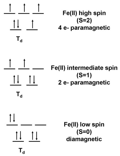
Figure 6.
Electron configurations and spin states for Fe(II) in tetrahedral coordination.
The CS varies with temperature mainly according to the second-order Doppler shift (SOD). Using the Debye model to describe the SOD, the temperature dependence of the center shift δ(T) can be expressed as
where δ0 is the isomer shift at 0 K and ΘM is the Mössbauer Debye temperature, which are the only two adjustable parameters [36], kB is the Boltzmann constant, m is the mass of the 57Fe nucleus, and c is the velocity of light. A series approximation to the Debye integral simplifies the calculation [37]. We fit the temperature dependence of the center shifts of various iron sulfides (Figure 7) and the parameters are given in Table 2. The presence of magnetic ordering in FeS1+x requires unpaired spins; hence, we rule out an LS configuration for this phase. Since the center shifts of FeS1+x and stoichiometric FeS are similar, there is unlikely to be a large change in electron density between the two phases; hence, we rule out an LS configuration for stoichiometric FeS as well. Kwon and coauthors [6] argued for strong itinerant spin fluctuations in stoichiometric mackinawite based on their observations of magnetic exchange energy splitting coupled with strongly delocalized 3d electrons. Our results support their conclusions and suggest that magnetic splitting in FeS1+x arises from a reduction in spin fluctuations due to excess sulfur either in the structure or on the surface. The low center shifts of stoichiometric FeS and FeS1+x compared to HS Fe2+ in FeS troilite (Figure 7) combined with the reduced magnetic moment of stoichiometric FeS observed using photoemission spectroscopy [6] suggest an IS electron configuration.
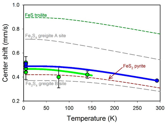
Figure 7.
Variation in iron sulfide center shifts with temperature. Data from this study are shown as filled circles in blue (singlet) and green (27 T sextet), with solid lines showing the fit to the Debye model. Literature values of center shifts were also fit to the Debye model and are shown as a green dashed line (FeS troilite [38]), brown dashed line (FeS2 pyrite [39,40]), and gray dashed line (Fe3S4 greigite [41]). Debye model parameters are given in Table 2.
Table 2.
Debye model parameters for iron sulfides.
4.3. Implications for Observing Mackinawite in the Environment
The Fe sulfide world is a world in flux. Many phases that form in low-temperature environments, including mackinawite and greigite, are thermodynamically unstable with respect to pyrite. These phases may participate in reactions that ultimately lead to pyrite formation, e.g., [9]. Temperature-dependent Mössbauer spectroscopy can help to identify the various mineral phases that are involved. Our results suggest that a single-line pattern represents pure mackinawite synthesized in the laboratory, but in natural environments, where impurities are more likely, the six-line pattern presented here assigned to FeS1+x may instead be more prevalent. A mineral transformation series may exist from pure mackinawite via FeS1+x to greigite. To shed more light on the structural stability and electronic properties of mackinawite, it would be valuable to collect temperature-dependent Mössbauer spectra of Ni-bearing mackinawite of magmatic origin, e.g., [28,29], and the cubic form of FeS, e.g., [42,43].
Author Contributions
Conceptualization, C.S., I.B.B. and S.P.; methodology, C.S., M.W. and I.B.B.; validation, C.S. and C.A.M.; formal analysis, C.S. and C.A.M.; investigation, C.S., M.W. and A.T.; resources, I.B.B., S.P. and C.A.M.; data curation, C.S.; writing—original draft preparation, C.S.; writing—review and editing, C.S., M.W., I.B.B., S.P., A.T. and C.A.M.; visualization, C.S. and C.A.M.; supervision, S.P. and C.A.M.; project administration, S.P.; funding acquisition, S.P. All authors have read and agreed to the published version of the manuscript.
Funding
This work was carried out in the framework of the research unit FOR 580, “Electron transfer processes in anoxic aquifers (e-TraP)”, funded by the Deutsche Forschungsgemeinschaft.
Acknowledgments
We thank Ayokunle Akindutire for help with mineral synthesis, George Luther III for fruitful discussions, and Anke Neumann for access to a Mössbauer spectrometer at the University of Newcastle.
Conflicts of Interest
The authors declare no conflict of interest. The funders had no role in the design of the study; in the collection, analyses, or interpretation of data; in the writing of the manuscript, and in the decision to publish the results.
References
- Rickard, D.; Luther, G.W. Chemistry of iron sulfides. Chem. Rev. 2007, 107, 514–562. [Google Scholar] [CrossRef] [PubMed]
- Hazen, R.M. Paleomineralogy of the Hadean Eon: A preliminary species list. Am. J. Sci. 2013, 313, 807–843. [Google Scholar] [CrossRef]
- Russell, M.J.; Hall, A.J. The emergence of life from iron monosulphide bubbles at a submarine hydrothermal redox and pH front. J. Geol. Soc. 1997, 154, 377–402. [Google Scholar] [CrossRef] [PubMed]
- White, L.M.; Bhartia, R.; Stucky, G.D.; Kanik, I.; Russell, M.J. Mackinawite and greigite in ancient alkaline hydrothermal chimneys: Identifying potential key catalysts for emergent life. Earth Planet. Sci. Lett. 2015, 430, 105–114. [Google Scholar] [CrossRef]
- Nakamura, R.; Okamoto, A.; Tajima, N.; Newton, G.J.; Kai, F.; Takashima, T.; Hashimoto, K. Biological iron-monosulfide production for efficient electricity harvesting from a deep-sea metal-reducing bacterium. ChemBioChem 2010, 11, 643–645. [Google Scholar] [CrossRef] [PubMed]
- Kwon, K.D.; Refson, K.; Bone, S.; Qiao, R.; Yang, W.-L.; Liu, Z.; Sposito, G. Magnetic ordering in tetragonal FeS: Evidence for strong itinerant spin fluctuations. Phys. Rev. B 2011, 83, 064402. [Google Scholar] [CrossRef]
- Lennie, A.R.; Redfern, S.A.T.; Schofield, P.F.; Vaughan, D.J. Synthesis and Rietveld crystal structure refinement of mackinawite, tetragonal FeS. Miner. Mag. 1995, 59, 677–683. [Google Scholar] [CrossRef]
- Csákberényi-Malasics, D.; Rodriguez-Blanco, J.D.; Kis, V.K.; Rečnik, A.; Benning, L.G.; Pósfai, M. Structural properties and transformations of precipitated FeS. Chem. Geol. 2012, 249–258. [Google Scholar] [CrossRef]
- Matamoros-Veloza, A.; Cespedes, O.; Johnson, B.R.G.; Stawski, T.M.; Terranova, U.; De Leeuw, N.H.; Benning, L.G. A highly reactive precursor in the iron sulfide system. Nat. Commun. 2018, 9, 1–7. [Google Scholar] [CrossRef]
- Mullet, M.; Boursiquot, S.; Abdelmoula, M.; Génin, J.-M.; Ehrhardt, J.-J. Surface chemistry and structural properties of mackinawite prepared by reaction of sulfide ions with metallic iron. Geochim. Cosmochim. Acta 2002, 66, 829–836. [Google Scholar] [CrossRef]
- Vaughan, D.J.; Craig, J.R. Mineral Chemistry of Metal Sulphides; Cambridge University Press: Cambridge, UK, 1978. [Google Scholar]
- Vaughan, D.; Ridout, M. Mössbauer studies of some sulphide minerals. J. Inorg. Nucl. Chem. 1971, 33, 741–746. [Google Scholar] [CrossRef]
- Gütlich, P.; Bill, E.; Trautwein, A. Mössbauer Spectroscopy and Transition Metal Chemistry; Springer: Berlin, Germany, 2011; p. 569. [Google Scholar]
- Gütlich, P.; Schröder, C. Mössbauer spectroscopy. In Methods in Physical Chemistry; Schäfer, R., Schmidt, P.C., Eds.; Wiley-VCH: Weinheim, Germany, 2012; Volume 2, pp. 351–389. [Google Scholar]
- Bertaut, E.; Burlet, P.; Chappert, J. Sur l’absence d’ordre magnetique dans la forme quadratique de FeS. Solid State Commun. 1965, 3, 335–338. [Google Scholar] [CrossRef]
- Bezdicka, P.; Grenier, J.-C.; Fournes, L.; Wattiaux, A.; Hagenmuller, P. Electrochemical formation of mackinawite FeS: An in situ Mössbauer resonance study. Eur. Solid State Inorg. Chem. 1989, 26, 353–365. [Google Scholar]
- Wan, M.; Schröder, C.; Peiffer, S. Fe(III):S(-II) concentration ratio controls the pathway and the kinetics of pyrite formation during sulfidation of ferric hydroxides. Geochim. Cosmochim. Acta 2017, 217, 334–348. [Google Scholar] [CrossRef]
- Morice, J.; Rees, L.; Rickard, D. Mössbauer studies of iron sulphides. J. Inorg. Nucl. Chem. 1969, 31, 3797–3802. [Google Scholar] [CrossRef]
- Devey, A.J.; Grau-Crespo, R.; De Leeuw, N.H. Combined density functional theory and interatomic potential study of the bulk and surface structures and properties of the iron sulfide mackinawite (FeS). J. Phys. Chem. C 2008, 112, 10960–10967. [Google Scholar] [CrossRef]
- Subedi, A.; Zhang, L.; Singh, D.J.; Du, M.-H. Density functional study of FeS, FeSe, and FeTe: Electronic structure, magnetism, phonons, and superconductivity. Phys. Rev. B 2008, 78, 134514. [Google Scholar] [CrossRef]
- Jacob, C.R.; Reiher, M. Spin in density-functional theory. Int. J. Quantum Chem. 2012, 112, 3661–3684. [Google Scholar] [CrossRef]
- Wan, M.; Shchukarev, A.; Lohmayer, R.; Planer-Friedrich, B.; Peiffer, S. Occurrence of surface polysulfides during the interaction between ferric (hydr)oxides and aqueous sulfide. Environ. Sci. Technol. 2014, 48, 5076–5084. [Google Scholar] [CrossRef]
- Schwertmann, U.; Cornell, R.M. Iron Oxides in the Laboratory, 2nd ed.; Wiley-VCH: Weinheim, Germany, 2000. [Google Scholar]
- Rancourt, D.; Ping, J. Voigt-based methods for arbitrary-shape static hyperfine parameter distributions in Mössbauer spectroscopy. Nucl. Instrum. Methods Phys. Res. Sect. B Beam Interact. Mater. At. 1991, 58, 85–97. [Google Scholar] [CrossRef]
- Patterson, R.R.; Fendorf, S.; Fendorf, M. Reduction of hexavalent chromium by amorphous iron sulfide. Environ. Sci. Technol. 1997, 31, 2039–2044. [Google Scholar] [CrossRef]
- Hellige, K.; Pollok, K.; Larese-Casanova, P.; Behrends, T.; Peiffer, S. Pathways of ferrous iron mineral formation upon sulfidation of lepidocrocite surfaces. Geochim. Cosmochim. Acta 2012, 81, 69–81. [Google Scholar] [CrossRef]
- Peiffer, S.; Behrends, T.; Hellige, K.; Larese-Casanova, P.; Wan, M.; Pollok, K. Pyrite formation and mineral transformation pathways upon sulfidation of ferric hydroxides depend on mineral type and sulfide concentration. Chem. Geol. 2015, 400, 44–55. [Google Scholar] [CrossRef]
- Evans, H.T.; Milton, C.; Chao, E.C.T.; Adler, I.; Mead, C.; Ingram, B.; Berner, R.A. Valleriite and the New Iron Sulfide, Mackinawite; U.S. Geological Survey Professional Paper 475-D; U.S. Geological Survey: Washington, DC, USA, 1964.
- Kouvo, O.; Vuorelainen, Y.; Long, J.V.P. A tetragonal iron sulfide. Am. Miner. 1963, 48, 511–524. [Google Scholar]
- Guilbaud, R.; Butler, I.B.; Ellam, R.M.; Rickard, D. Fe isotope exchange between Fe(II)aq and nanoparticulate mackinawite (FeSm) during nanoparticle growth. Earth Planet. Sci. Lett. 2010, 300, 174–183. [Google Scholar] [CrossRef]
- Roberts, A.P.; Chang, L.; Rowan, C.J.; Horng, C.-S.; Florindo, F. Magnetic properties of sedimentary greigite (Fe3S4): An update. Rev. Geophys. 2011, 49. [Google Scholar] [CrossRef]
- Stanjek, H. Comparison of pedogenic and sedimentary greigite by X-ray Diffraction and Mössbauer spectroscopy. Clays Clay Miner. 1994, 42, 451–454. [Google Scholar] [CrossRef]
- Vandenberghe, R.E.; De Grave, E.; De Bakker, P.M.A.; Krs, M.; Hus, J.J. Mössbauer effect study of natural greigite. Hyperfine Interact. 1992, 68, 319–322. [Google Scholar] [CrossRef]
- Kim, W.; Park, I.J.; Kim, C.S. Mössbauer study of magnetic structure of cation-deficient iron sulfide Fe0.92S. J. Appl. Phys. 2009, 105, 7. [Google Scholar] [CrossRef]
- Ok, H.N. Relaxation effects in antiferromagnetic ferrous carbonate. Phys. Rev. 1969, 185, 472–476. [Google Scholar] [CrossRef]
- Pound, R.V.; Rebka, J.A., Jr. Variation with temperature of the energy of recoil-free gamma rays from solids. Phys. Rev. Lett. 1960, 4, 274–277. [Google Scholar] [CrossRef]
- Heberle, J. The Debye integrals, the thermal shift and the Mössbauer fraction. In Mössbauer Effect Methodology; Gruverman, I.J., Ed.; Springer: Boston, MA, USA, 1971; Volume 7, pp. 299–308. [Google Scholar]
- Hafner, S.S.; Kalvius, G.M. The Mössbauer resonance of Fe57 in troilite (FeS) and pyrrhotite (Fe0.88S). Z. Krist. 1966, 123, 443–458. [Google Scholar] [CrossRef]
- Montano, P.; Seehra, M. Magnetism of iron pyrite (FeS2)—A Mössbauer study in an external magnetic field. Solid State Commun. 1976, 20, 897–898. [Google Scholar] [CrossRef]
- Temperley, A.; Lefevre, H. The Mössbauer effect in marcasite structure iron compounds. J. Phys. Chem. Solids 1966, 27, 85–92. [Google Scholar] [CrossRef]
- Spender, M.R.; Coey, J.M.D.; Morrish, A.H. The magnetic properties and Mössbauer spectra of synthetic samples of Fe3S4. Can. J. Phys. 1972, 50, 2313–2326. [Google Scholar] [CrossRef]
- De Médicis, R. Cubic FeS, a metastable iron sulfide. Science 1970, 170, 1191–1192. [Google Scholar] [CrossRef]
- Takeno, S.; Zôka, H.; Niihara, T. Metastable cubic iron sulfide—With special reference to mackinawite. Am. Miner. 1970, 55, 1639–1649. [Google Scholar]
Publisher’s Note: MDPI stays neutral with regard to jurisdictional claims in published maps and institutional affiliations. |
© 2020 by the authors. Licensee MDPI, Basel, Switzerland. This article is an open access article distributed under the terms and conditions of the Creative Commons Attribution (CC BY) license (http://creativecommons.org/licenses/by/4.0/).