Loop Representation of Wigner’s Little Groups

Abstract

Wigner’s little groups are the subgroups of the Lorentz group whose transformations leave the momentum of a given particle invariant. They thus define the internal space-time symmetries of relativistic particles. These symmetries take different mathematical forms for massive and for massless particles. However, it is shown possible to construct one unified representation using a graphical description. This graphical approach allows us to describe vividly parity, time reversal, and charge conjugation of the internal symmetry groups. As for the language of group theory, the two-by-two representation is used throughout the paper. While this two-by-two representation is for spin-1/2 particles, it is shown possible to construct the representations for spin-0 particles, spin-1 particles, as well as for higher-spin particles, for both massive and massless cases. It is shown also that the four-by-four Dirac matrices constitute a two-by-two representation of Wigner’s little group.

1. Introduction

In his 1939 paper [1], Wigner introduced subgroups of the Lorentz group whose transformations leave the momentum of a given particle invariant. These subgroups are called Wigner’s little groups in the literature and are known as the symmetry groups for internal space-time structure.

For instance, a massive particle at rest can have spin that can be rotated in three-dimensional space. The little group in this case is the three-dimensional rotation group. For a massless particle moving along the z direction, Wigner noted that rotations around the z axis do not change the momentum. In addition, he found two more degrees of freedom, which together with the rotation, constitute a subgroup locally isomorphic to the two-dimensional Euclidean group.

However, Wigner’s 1939 paper did not deal with the following critical issues.

• As for the massive particle, Wigner worked out his little group in the Lorentz frame where the particle is at rest with zero momentum, resulting in the three-dimensional rotation group. He could have Lorentz-boosted the $O\left(3\right)$-like little group to make the little group for a moving particle.
• While the little group for a massless particle is like $E\left(2\right)$, it is not difficult to associate the rotational degree of freedom to the helicity. However, Wigner did not give physical interpretations to the two translation-like degrees of freedom.
• While the Lorentz group does not allow mass variations, particles with infinite momentum should behave like massless particles. The question is whether the Lorentz-boosted $O\left(3\right)$-like little group becomes the $E\left(2\right)$-like little group for particles with infinite momentum.

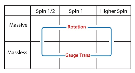
These issues have been properly addressed since then [2,3,4,5]. The translation-like degrees of freedom for massless particles collapse into one gauge degree of freedom, and the $E\left(2\right)$-like little group can be obtained as the infinite-momentum limit of the $O\left(3\right)$-like little group. This history is summarized in Figure 1.

In this paper, we shall present these developments using a mathematical language more transparent than those used in earlier papers.

• In his original paper [1], Wigner worked out his little group for the massive particle when its momentum is zero. How about moving massive particles? In this paper, we start with a moving particle with non-zero momentum. We then perform rotations and boosts whose net effect does not change the momentum [6,7,8]. This procedure can be applied to the massive, massless, and imaginary-mass cases.
• By now, we have a clear understanding of the group $SL(2,c)$ as the universal covering group of the Lorentz group. The logic with two-by-two matrices is far more transparent than the mathematics based on four-by-four matrices. We shall thus use the two-by-two representation of the Lorentz group throughout the paper [5,9,10,11].

The purpose of this paper is to make the physics contained in Wigner’s original paper more transparent. In Section 2, we give the six generators of the Lorentz group. It is possible to write them in terms of coordinate transformations, four-by-four matrices, and two-by-two matrices. In Section 3, we introduce Wigner’s little groups in terms of two-by-two matrices. In Section 4, it is shown possible to construct transformation matrices of the little group by performing rotations and a boost resulting in a non-trivial matrix, which leaves the given momentum invariant.

Since we are more familiar with Dirac matrices than the Lorentz group, it is shown in Section 5 that Dirac matrices are a representation of the Lorentz group, and his four-by-four matrices are two-by-two representations of the two-by-two representation of Wigner’s little groups. In Section 6, we construct spin-0 and spin-1 particles for the SL(2,c) spinors. We also discuss massless higher spin particles.

2. Lorentz Group and Its Representations

The group of four-by-four matrices, which performs Lorentz transformations on the four-dimensional Minkowski space leaving invariant the quantity $\left(t^2-z^2-x^2-y^2\right)$, forms the starting point for the Lorentz group. As there are three rotation and three boost generators, the Lorentz group is a six-parameter group.

Einstein, by observing that this Lorentz group also leaves invariant $\left(E,p_z,p_x,p_y\right)$, was able to derive his Lorentz-covariant energy-momentum relation commonly known as $E=m{c}^2$. Thus, the particle mass is a Lorentz-invariant quantity.

The Lorentz group is generated by the three rotation operators:

$$J_i=-i\left(x_j\frac{\partial }{\partial x_k}-x_k\frac{\partial }{\partial x_j}\right),$$

(1)

where $i,j,k=1,2,3$, and three boost operators:

$$K_i=-i\left(t\frac{\partial }{\partial x_i}+x_i\frac{\partial }{\partial t}\right).$$

(2)

These generators satisfy the closed set of commutation relations:

$$\left[J_i,J_j\right]=i{ϵ}_{ijk}{J}_k,\left[J_i,K_j\right]=i{ϵ}_{ijk}{K}_k,\left[K_i,K_j\right]=-i{ϵ}_{ijk}{J}_k,$$

(3)

which are known as the Lie algebra for the Lorentz group.

Under the space inversion, $x_i\to -x_i$, or the time reflection, $t\to -t$, the boost generators $K_i$ change sign. However, the Lie algebra remains invariant, which means that the commutation relations remain invariant under Hermitian conjugation.

In terms of four-by-four matrices applicable to the Minkowskian coordinate of $(t,z,x,y)$, the generators can be written as:

$$J_3=\left(\begin{array}{cccc}0& 0& 0& 0\\ 0& 0& 0& 0\\ 0& 0& 0& -i\\ 0& 0& i& 0\end{array}\right),K_3=\left(\begin{array}{cccc}0& i& 0& 0\\ i& 0& 0& 0\\ 0& 0& 0& 0\\ 0& 0& 0& 0\end{array}\right),$$

(4)

for rotations around and boosts along the z direction, respectively. Similar expressions can be written for the x and y directions. We see here that the rotation generators $J_i$ are Hermitian, but the boost generators $K_i$ are anti-Hermitian.

We can also consider the two-by-two matrices:

$$J_i=\frac{1}{2}{\sigma }_i,\mathrm{and}{K}_i=\frac{i}{2}{\sigma }_i,$$

(5)

where ${\sigma }_i$ are the Pauli spin matrices. These matrices also satisfy the commutation relations given in Equation (3).

There are interesting three-parameter subgroups of the Lorentz group. In 1939 [1], Wigner considered the subgroups whose transformations leave the four-momentum of a given particle invariant. First of all, consider a massive particle at rest. The momentum of this particle is invariant under rotations in three-dimensional space. What happens for the massless particle that cannot be brought to a rest frame? In this paper we shall consider this and other problems using the two-by-two representation of the Lorentz group.

3. Two-by-Two Representation of Wigner’s Little Groups

The six generators of Equation (5) lead to the group of two-by-two unimodular matrices of the form:

$$G=\left(\begin{array}{cc}\alpha & \beta \\ \gamma & \delta \end{array}\right),$$

(6)

with $det\left(G\right)=1$, where the matrix elements are complex numbers. There are thus six independent real numbers to accommodate the six generators given in Equation (5). The groups of matrices of this form are called $SL(2,c)$ in the literature. Since the generators $K_i$ are not Hermitian, the matrix G is not always unitary. Its Hermitian conjugate is not necessarily the inverse.

The space-time four-vector can be written as [5,9,11]:

$$\left(\begin{array}{cc}t+z& x-iy\\ x+iy& t-z\end{array}\right),$$

(7)

whose determinant is $t^2-z^2-x^2-z^2$, and remains invariant under the Hermitian transformation:

$$X^{\prime }=GX{G}^{†}.$$

(8)

This is thus a Lorentz transformation. This transformation can be explicitly written as:

$$\left(\begin{array}{cc}{t}^{\prime }+z^{\prime }& x^{\prime }-i{y}^{\prime }\\ x^{\prime }+i{y}^{\prime }& t^{\prime }-z^{\prime }\end{array}\right)=\left(\begin{array}{cc}\alpha & \beta \\ \gamma & \delta \end{array}\right)\left(\begin{array}{cc}t+z& x-iy\\ x+iy& t-z\end{array}\right)\left(\begin{array}{cc}{\alpha }^{*}& {\gamma }^{*}\\ {\beta }^{*}& {\delta }^{*}\end{array}\right).$$

(9)

With these six independent real parameters, it is possible to construct four-by-four matrices for Lorentz transformations applicable to the four-dimensional Minkowskian space [5,12]. For the purpose of the present paper, we need some special cases, and they are given in

Table 1. Two-by-two and four-by-four representations of the Lorentz group.

Generators	Two-by-Two	Four-by-Four
$J_3=\frac{1}{2}\left(\begin{array}{cc}1& 0\\ 0& -1\end{array}\right)$	$\left(\begin{array}{cc}exp(i\varphi /2)& 0\\ 0& exp(-i\varphi /2)\end{array}\right)$	$\left(\begin{array}{cccc}1& 0& 0& 0\\ 0& 1& 0& 0\\ 0& 0& cos\varphi & -sin\varphi \\ 0& 0& sin\varphi & cos\varphi \end{array}\right)$
$K_3=\frac{1}{2}\left(\begin{array}{cc}i& 0\\ 0& -i\end{array}\right)$	$\left(\begin{array}{cc}exp(\eta /2)& 0\\ 0& exp(-\eta /2)\end{array}\right)$	$\left(\begin{array}{cccc}cosh\eta & sinh\eta & 0& 0\\ sinh\eta & cosh\eta & 0& 0\\ 0& 0& 1& 0\\ 0& 0& 0& 1\end{array}\right)$
$J_1=\frac{1}{2}\left(\begin{array}{cc}0& 1\\ 1& 0\end{array}\right)$	$\left(\begin{array}{cc}cos(\theta /2)& isin(\theta /2)\\ isin(\theta /2)& cos(\theta /2)\end{array}\right)$	$\left(\begin{array}{cccc}1& 0& 0& 0\\ 0& cos\theta & 0& sin\theta \\ 0& 0& 1& 0\\ 0& -sin\theta & 0& cos\theta \end{array}\right)$
$K_1=\frac{1}{2}\left(\begin{array}{cc}0& i\\ i& 0\end{array}\right)$	$\left(\begin{array}{cc}cosh(\lambda /2)& sinh(\lambda /2)\\ sinh(\lambda /2)& cosh(\lambda /2)\end{array}\right)$	$\left(\begin{array}{cccc}cosh\lambda & 0& sinh\lambda & 0\\ 0& 1& 0\\ sinh\lambda & 0& cosh\lambda & 0\\ 0& 0& 0& 1\end{array}\right)$
$J_2=\frac{1}{2}\left(\begin{array}{cc}0& -i\\ i& 0\end{array}\right)$	$\left(\begin{array}{cc}cos(\theta /2)& -sin(\theta /2)\\ sin(\theta /2)& cos(\theta /2)\end{array}\right)$	$\left(\begin{array}{cccc}1& 0& 0& 0\\ 0& cos\theta & -sin\theta & 0\\ 0& sin\theta & cos\theta & 0\\ 0& 0& 0& 1\end{array}\right)$
$K_2=\frac{1}{2}\left(\begin{array}{cc}0& 1\\ -1& 0\end{array}\right)$	$\left(\begin{array}{cc}cosh(\lambda /2)& -isinh(\lambda /2)\\ isinh(\lambda /2)& cosh(\lambda /2)\end{array}\right)$	$\left(\begin{array}{cccc}cosh\lambda & 0& 0& sinh\lambda \\ 0& 1& 0& 0\\ 0& 0& 1& 0\\ sinh\lambda & 0& 0& cosh\lambda \end{array}\right)$

.

Likewise, the two-by-two matrix for the four-momentum takes the form:

$$P=\left(\begin{array}{cc}{p}_0+p_z& p_x-i{p}_y\\ p_x+i{p}_y& p_0-p_z\end{array}\right),$$

(10)

with $p_0=\sqrt{m^2+p_z^2+p_x^2+p_2^2}.$ The transformation property of Equation (9) is applicable also to this energy-momentum four-vector.

In 1939 [1], Wigner considered the following three four-vectors.

$$P_{+}=\left(\begin{array}{cc}1& 0\\ 0& 1\end{array}\right),P_0=\left(\begin{array}{cc}1& 0\\ 0& 0\end{array}\right),P_{-}=\left(\begin{array}{cc}1& 0\\ 0& -1\end{array}\right).$$

(11)

whose determinants are 1, 0, and −1, respectively, corresponding to the four-momenta of massive, massless, and imaginary-mass particles, as shown in

Table 2. The Wigner momentum vectors in the two-by-two matrix representation together with the corresponding transformation matrix. These four-momentum matrices have determinants that are positive, zero, and negative for massive, massless, and imaginary-mass particles, respectively.

Particle Mass	Four-Momentum	Transform Matrix
Massive	$\left(\begin{array}{cc}1& 0\\ 0& 1\end{array}\right)$	$\left(\begin{array}{cc}cos(\theta /2)& -sin(\theta /2)\\ sin(\theta /2)& cos(\theta /2)\end{array}\right)$
Massless	$\left(\begin{array}{cc}1& 0\\ 0& 0\end{array}\right)$	$\left(\begin{array}{cc}1& -\gamma \\ 0& 1\end{array}\right)$
Imaginary mass	$\left(\begin{array}{cc}1& 0\\ 0& -1\end{array}\right)$	$\left(\begin{array}{cc}cosh(\lambda /2)& sinh(\lambda /2)\\ sinh(\lambda /2)& cosh(\lambda /2)\end{array}\right)$

.

He then constructed the subgroups of the Lorentz group whose transformations leave these four-momenta invariant. These subgroups are called Wigner’s little groups in the literature. Thus, the matrices of these little groups should satisfy:

$$W{P}_i{W}^{†}=P_i,$$

(12)

where $i=+,0,-$. Since the momentum of the particle is fixed, these little groups define the internal space-time symmetries of the particle. For all three cases, the momentum is invariant under rotations around the z axis, as can be seen from the expression given for the rotation matrix generated by $J_3$ given in Table 1.

For the first case corresponding to a massive particle at rest, the requirement of the subgroup is:

$$W{P}_{+}{W}^{†}=P_{+}.$$

(13)

This requirement tells that the subgroup is the rotation subgroup with the rotation matrix around the y direction:

$$R\left(\theta \right)=\left(\begin{array}{cc}cos(\theta /2)& -sin(\theta /2)\\ sin(\theta /2)& cos(\theta /2)\end{array}\right).$$

(14)

For the second case of $P_0$, the triangular matrix of the form:

$$\mathsf{\Gamma }\left(\xi \right)=\left(\begin{array}{cc}1& -\xi \\ 0& 1\end{array}\right),$$

(15)

satisfies the Wigner condition of Equation (12). If we allow rotations around the z axis, the expression becomes:

$$\mathsf{\Gamma }(\xi ,\varphi )=\left(\begin{array}{cc}1& -\xi exp(-i\varphi )\\ 0& 1\end{array}\right).$$

(16)

This matrix is generated by:

$$N_1=J_2-K_1=\left(\begin{array}{cc}0& -i\\ 0& 0\end{array}\right),\mathrm{and}{N}_2=J_1+K_2=\left(\begin{array}{cc}0& 1\\ 0& 0\end{array}\right).$$

(17)

Thus, the little group is generated by $J_3$, $N_1$, and $N_2$. They satisfy the commutation relations:

$$\left[N_1,N_2\right]=0,\left[J_3,N_1\right]=i{N}_2,\left[J_3,K_2\right]=-i{N}_1.$$

(18)

Wigner in 1939 [1] observed that this set is the same as that of the two-dimensional Euclidean group with one rotation and two translations. The physical interpretation of the rotation is easy to understand. It is the helicity of the massless particle. On the other hand, the physics of the $N_1$ and $N_2$ matrices has a stormy history, and the issue was not completely settled until 1990 [4]. They generate gauge transformations.

For the third case of $P_{-}$, the matrix of the form:

$$S\left(\lambda \right)=\left(\begin{array}{cc}cosh(\lambda /2)& sinh(\lambda /2)\\ sinh(\lambda /2)& cosh(\lambda /2)\end{array}\right),$$

(19)

satisfies the Wigner condition of Equation (12). This corresponds to the Lorentz boost along the x direction generated by $K_1$ as shown in Table 1. Because of the rotation symmetry around the z axis, the Wigner condition is satisfied also by the boost along the y axis. The little group is thus generated by $J_3,K_1$, and $K_2$. These three generators:

$$\left[J_3,K_1\right]=i{K}_2,\left[J_3,K_2\right]=-i{K}_1,\left[K_1,K_2\right]=-i{J}_3$$

(20)

form the little group $O(2,1)$, which is the Lorentz group applicable to two space-like and one time-like dimensions.

Of course, we can add rotations around the z axis. Let us Lorentz-boost these matrices along the z direction with the diagonal matrix:

$$B\left(\eta \right)=\left(\begin{array}{cc}exp(\eta /2)& 0\\ 0& exp(-\eta /2)\end{array}\right).$$

(21)

Then, the matrices of Equations (14), (15), and (19) become:

$$B\left(\eta \right)R\left(\theta \right)B(-\eta )=\left(\begin{array}{cc}cos(\theta /2)& -e^{\eta }sin(\theta /2)\\ e^{-\eta }sin(\theta /2)& cos(\theta /2)\end{array}\right),$$

(22)

$$B\left(\eta \right)\mathsf{\Gamma }\left(\xi \right)B(-\eta )=\left(\begin{array}{cc}1& -e^{\eta }\xi \\ 0& 1\end{array}\right),$$

(23)

$$B\left(\eta \right)S(-\lambda )B(-\eta )=\left(\begin{array}{cc}cosh(\lambda /2)& -e^{\eta }sinh(\lambda /2)\\ -e^{-\eta }sinh(\lambda /2)& cosh(\lambda /2)\end{array}\right),$$

(24)

respectively. We have changed the sign of $\lambda$ for future convenience.

When $\eta$ becomes large, $\theta ,\xi$, and $\lambda$ should become small if the upper-right elements of the these three matrices are to remain finite. In that case, the diagonal elements become one, and all three matrices become like the triangular matrix:

$$\left(\begin{array}{cc}1& -\gamma \\ 0& 1\end{array}\right).$$

(25)

Here comes the question of whether the matrix of Equation (24) can be continued from Equation (22), via Equation (23). For this purpose, let us write Equation (22) as:

$$\left(\begin{array}{cc}1-{\left(\gamma ϵ\right)}^2/2& -\gamma \\ \gamma {ϵ}^2& 1-{\left(\gamma ϵ\right)}^2/2\end{array}\right),$$

(26)

for small $\theta =2\gamma ϵ$, with $ϵ=e^{-\eta }$. For Equation (24), we can write:

$$\left(\begin{array}{cc}1+{\left(\gamma ϵ\right)}^2/2& -\gamma \\ -\gamma {ϵ}^2& 1+{\left(\gamma ϵ\right)}^2/2\end{array}\right),$$

(27)

with $\lambda =-2\gamma ϵ.$ Both of these expressions become the triangular matrix of Equation (25) when $ϵ=0$.

For small values of $ϵ$, the diagonal elements change from $cos(\theta /2)$ to $cosh(\lambda /2)$ while $sin(\theta /2)$ becomes $-sinh(\lambda /2)$. Thus, it is possible to continue from Equation (22) to Equation (24). The mathematical details of this process have been discussed in our earlier paper on this subject [13].

We are then led to the question of whether there is one expression that will take care of all three cases. We shall discuss this issue in Section 4.

4. Loop Representation of Wigner’s Little Groups

It was noted in Section 3 that matrices of Wigner’s little group take different forms for massive, massless, and imaginary-mass particles. In this section, we construct one two-by-two matrix that works for all three different cases.

In his original paper [1], Wigner constructs those matrices in specific Lorentz frames. For instance, for a moving massive particle with a non-zero momentum, Wigner brings it to the rest frame and works out the $O\left(3\right)$ subgroup of the Lorentz group as the little group for this massive particle. In order to complete the little group, we should boost this $O\left(3\right)$ to the frame with the original non-zero momentum [4].

In this section, we construct transformation matrices without changing the momentum. Let us assume that the momentum is along the z direction; the rotation around the z axis leaves the momentum invariant. According to the Euler decomposition, the rotation around the y axis, in addition, will accommodate rotations along all three directions. For this reason, it is enough to study what happens in transformations within the $xz$ plane [14].

It was Kupersztych [6] who showed in 1976 that it is possible to construct a momentum-preserving transformation by a rotation followed by a boost as shown in Figure 2. In 1981 [7], Han and Kim showed that the boost can be decomposed into two components as illustrated in Figure 2. In 1988 [8], Han and Kim showed that the same purpose can be achieved by one boost preceded and followed by the same rotation matrix, as shown also in Figure 2. We choose to call this loop the “D loop” and write the transformation matrix as:

$$D(\alpha ,\chi )=R\left(\alpha \right)S(-2\chi )R\left(\alpha \right).$$

(28)

The D matrix can now be written as three matrices. This form is known in the literature as the Bargmann decomposition [10]. This form gives additional convenience. When we take the inverse or the Hermitian conjugate, we have to reverse the order of matrices. However, this particular form does not require re-ordering.

The D matrix of Equation (28) becomes:

$$D(\alpha ,\chi )=\left(\begin{array}{cc}(cos\alpha )cosh\chi & -sinh\chi -(sin\alpha )cosh\chi \\ -sinh\chi +(sin\alpha )cosh\chi & (cos\alpha )cosh\chi \end{array}\right).$$

(29)

If the diagonal element is smaller than one with $\left(\right(cos\alpha )cosh\chi )<1$, the off-diagonal elements have opposite signs. Thus, this D matrix can serve as the Wigner matrix of Equation (22) for massive particles. If the diagonal elements are one, one of the off-diagonal elements vanishes, and this matrix becomes triangular like Equation (23). If the diagonal elements are greater than one with $\left(\right(cos\alpha )cosh\chi )>1$, this matrix can become Equation (24). In this way, the matrix of Equation (28) can accommodate the three different expressions given in Equations (22)–(24).

4.1. Continuity Problems

Let us go back to the three separate formulas given in Equations (22)–(24). If $\eta$ becomes infinity, all three of them become triangular. For the massive particle, $tanh\eta$ is the particle speed, and:

$$tanh\eta =\frac{p}{p_0},$$

(30)

where p and $p_0$ are the momentum and energy of the particle, respectively.

When the particle is massive with $m^2>0$, the ratio:

$$\frac{\mathrm{lower}-\mathrm{left}\mathrm{element}}{\mathrm{upper}-\mathrm{right}\mathrm{element}},$$

(31)

is negative and is:

$$-e^{-2\eta }=\frac{1-\sqrt{1+m^2/p^2}}{1+\sqrt{1+m^2/p^2}}.$$

(32)

If the mass is imaginary with $m^2<0$, the ratio is positive and:

$$e^{-2\eta }=\frac{1-\sqrt{1+m^2/p^2}}{1+\sqrt{1+m^2/p^2}}.$$

(33)

This ratio is zero for massless particles. This means that when $m^2$ changes from positive to negative, the ratio changes from $-e^{-2\eta }$ to $e^{-2\eta }$. This transition is continuous, but not analytic. This aspect of non-analytic continuity has been discussed in one of our earlier papers [13].

The D matrix of Equation (29) combines all three matrices given in Equations (22)–(24) into one matrix. For this matrix, the ratio of Equation (31) becomes:

$$\frac{tanh\chi -sin\alpha }{tanh\chi +sin\alpha }=\frac{1-\sqrt{1+{(m/p)}^2}}{1+\sqrt{1+(m/p^2)}}.$$

(34)

Thus,

$$\frac{m^2}{p^2}={\left(\frac{sin\alpha }{tanh\chi }\right)}^2-1.$$

(35)

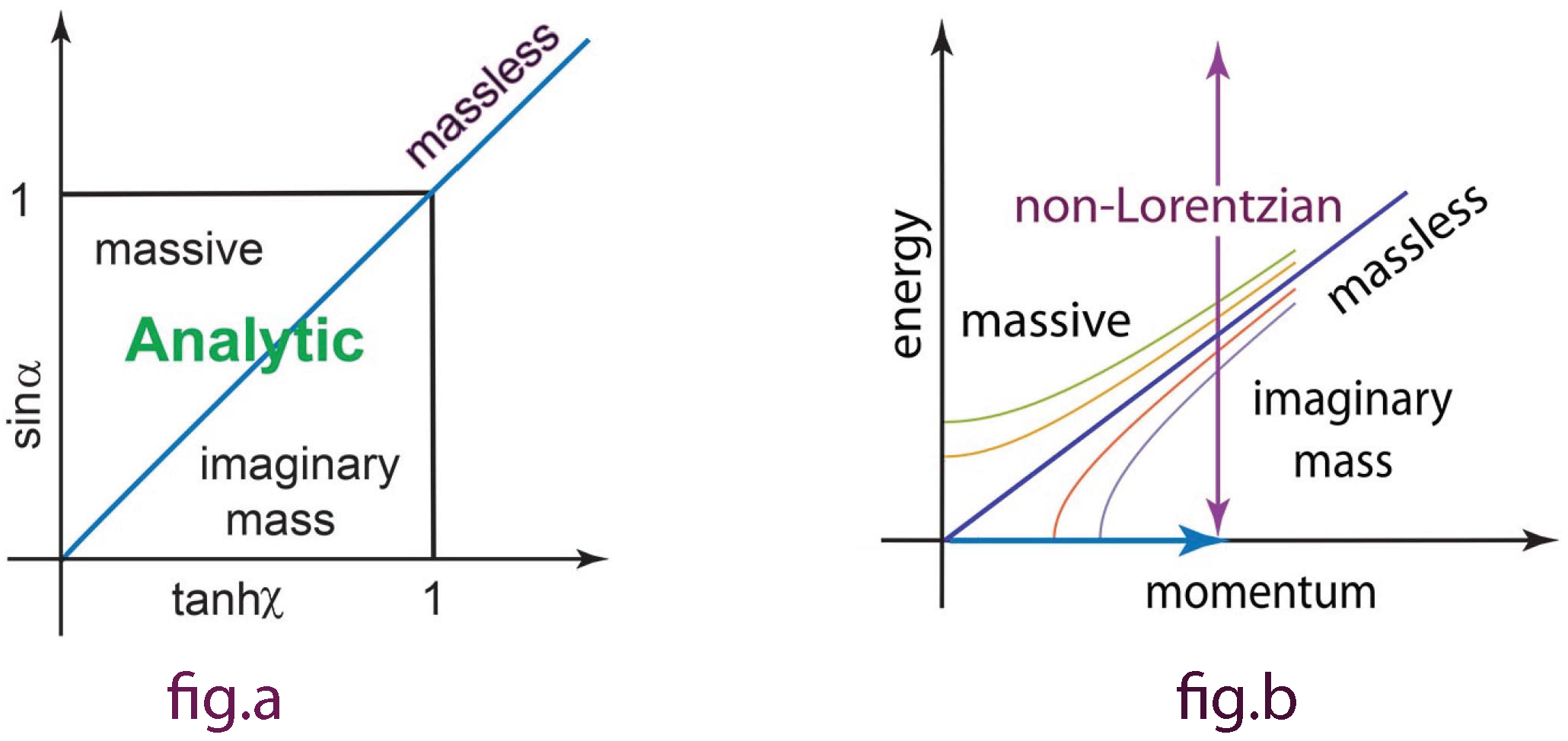
For the D loop of Figure 2, both $tanh\chi$ and $sin\alpha$ range from 0–1, as illustrated in Figure 3.

For small values of the mass for a fixed value of the momentum, this expression becomes:

$$-\frac{m^2}{4p^2}.$$

(36)

Thus, the change from positive values of $m^2$ to negative values is continuous and analytic. For massless particles, $m^2$ is zero, while it is negative for imaginary-mass particles.

We realize that the mass cannot be changed within the frame of the Lorentz group and that both $\alpha$ and $\eta$ are parameters of the Lorentz group. On the other hand, their combinations according to the D loop of Figure 2 can change the value of $m^2$ according to Equation (35) and Figure 3.

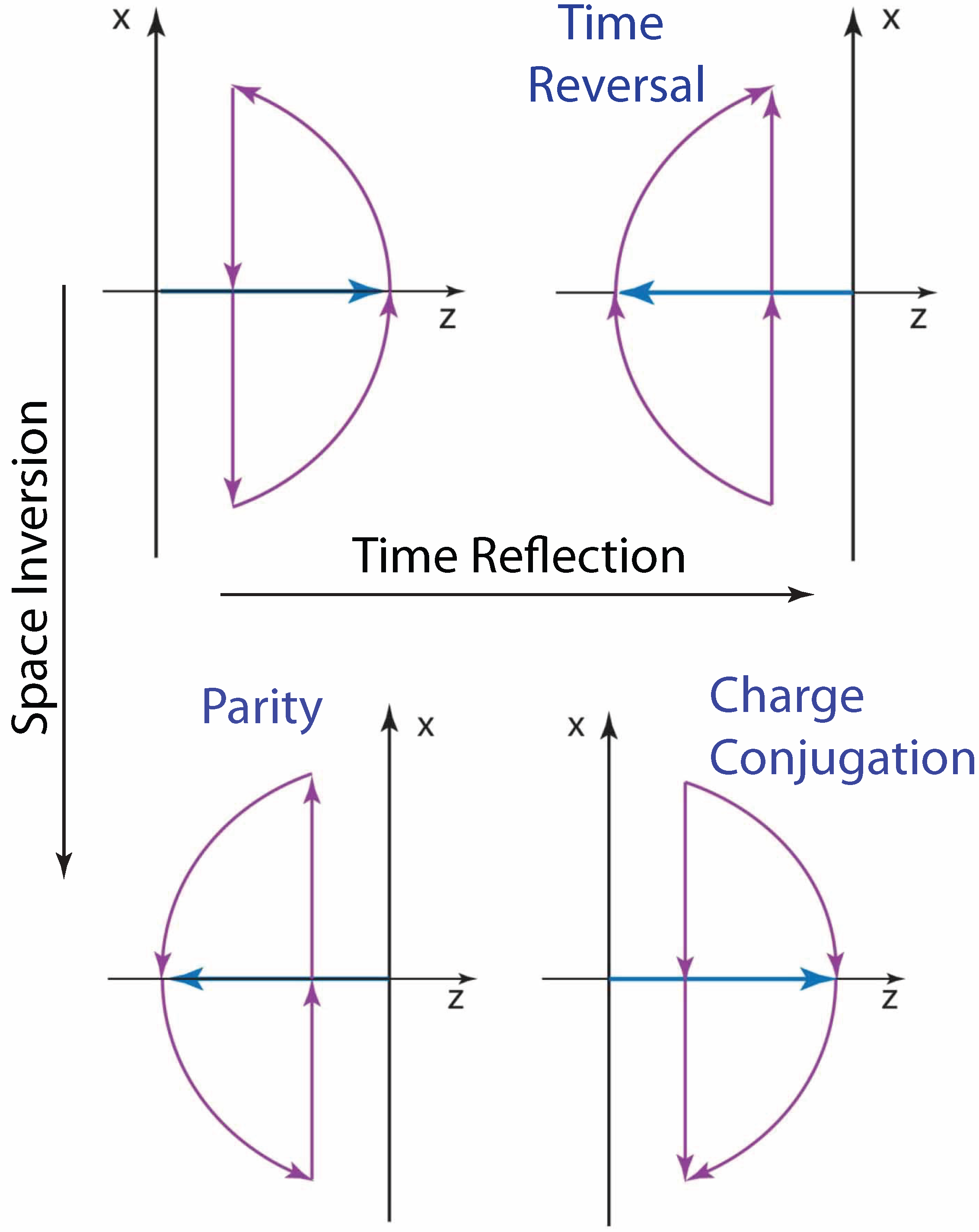
4.2. Parity, Time Reversal, and Charge Conjugation

Space inversion leads to the sign change in $\chi$:

$$D(\alpha ,-\chi )=\left(\begin{array}{cc}(cos\alpha )cosh\chi & sinh\chi -(sin\alpha )cosh\chi \\ sinh\chi +(sin\alpha )cosh\chi & (cos\alpha )cosh\chi \end{array}\right),$$

(37)

and time reversal leads to the sign change in both $\alpha$ and $\chi$:

$$D(-\alpha ,-\chi )=\left(\begin{array}{cc}(cos\alpha )cosh\chi & sinh\chi +(sin\alpha )cosh\chi \\ sinh\chi -(sin\alpha )cosh\chi & (cos\alpha )cosh\chi \end{array}\right).$$

(38)

If we space-invert this expression, the result is a change only in the direction of rotation,

$$D(-\alpha ,\chi )=\left(\begin{array}{cc}(cos\alpha )cosh\chi & -sinh\chi +(sin\alpha )cosh\chi \\ -sinh\chi -(sin\alpha )cosh\chi & (cos\alpha )cosh\chi \end{array}\right).$$

(39)

The combined transformation of space inversion and time reversal is known as the “charge conjugation”. All of these transformations are illustrated in Figure 4.

Let us go back to the Lie algebra of Equation (3). This algebra is invariant under Hermitian conjugation. This means that there is another set of commutation relations,

$$\left[J_i,J_j\right]=i{ϵ}_{ijk}{J}_k,\left[J_i,{\dot{K}}_j\right]=i{ϵ}_{ijk}{\dot{K}}_k,\left[{\dot{K}}_i,{\dot{K}}_j\right]=-i{ϵ}_{ijk}{J}_k,$$

(40)

where $K_i$ is replaced with ${\dot{K}}_i=-K_i.$ Let us go back to the expression of Equation (2). This transition to the dotted representation is achieved by the space inversion or by the parity operation.

On the other hand, the complex conjugation of the Lie algebra of Equation (3) leads to:

$$\left[J_i^{*},J_j^{*}\right]=-i{ϵ}_{ijk}{J}_k^{*},\left[J_i^{*},K_j^{*}\right]=-i{ϵ}_{ijk}{K}_k^{*},\left[K_i^{*},K_j^{*}\right]=i{ϵ}_{ijk}{J}_k^{*}.$$

(41)

It is possible to restore this algebra to that of the original form of Equation (3) if we replace $J_i^{*}$ by $-J_i$ and $K_i^{*}$ by $-K_i$. This corresponds to the time-reversal process. This operation is known as the anti-unitary transformation in the literature [15,16].

Since the algebras of Equations (3) and (41) are invariant under the sign change of $K_i$ and $K_i^{*}$, respectively, there is another Lie algebra with $J_i^{*}$ replaced by $-Ji$ and $K_i^{*}$ by $-{\dot{K}}_i$. This is the parity operation followed by time reversal, resulting in charge conjugation. With the four-by-four matrices for spin-1 particles, this complex conjugation is trivial, and $J_i^{*}=-J_i$, as well as $K_i^{*}=-K_i.$

On the other hand, for spin $1/2$ particles, we note that:

$$\begin{array}{c}{J}_1^{*}=J_1,J_2^{*}=-J_2,J_3^{*}=J_3,\hfill \\ K_1^{*}=-K_1,K_2^{*}=K_2,K_3^{*}=-K_3.\hfill \end{array}$$

(42)

Thus, $J_i^{*}$ should be replaced by ${\sigma }_2{J}_i{\sigma }_2$, and $K_i^{*}$ by -${\sigma }_2{K}_i{\sigma }_2$.

5. Dirac Matrices as a Representation of the Little Group

The Dirac equation, Dirac matrices, and Dirac spinors constitute the basic language for spin-1/2 particles in physics. Yet, they are not widely recognized as the package for Wigner’s little group. Yes, the little group is for spins, so are the Dirac matrices.

Let us write the Dirac equation as:

$$(p·\gamma -m)\psi (\overrightarrow{x},t)=\lambda \psi (\overrightarrow{x},t).$$

(43)

This equation can be explicitly written as:

$$\left(-i{\gamma }_0\frac{\partial }{\partial t}-i{\gamma }_1\frac{\partial }{\partial x}-i{\gamma }_2\frac{\partial }{\partial y}-i{\gamma }_3\frac{\partial }{\partial z}-m\right)\psi (\overrightarrow{x},t)=\lambda \psi (\overrightarrow{x},t),$$

(44)

where:

$${\gamma }_0=\left(\begin{array}{cc}0& I\\ I& 0\end{array}\right),{\gamma }_1=\left(\begin{array}{cc}0& {\sigma }_1\\ -{\sigma }_1& 0\end{array}\right),{\gamma }_2=\left(\begin{array}{cc}0& {\sigma }_2\\ -{\sigma }_2& 0\end{array}\right),{\gamma }_3=\left(\begin{array}{cc}0& {\sigma }_3\\ -{\sigma }_3& 0\end{array}\right),$$

(45)

where I is the two-by-two unit matrix. We use here the Weyl representation of the Dirac matrices.

The Dirac spinor has four components. Thus, we write the wave function for a free particle as:

$$\psi (\overrightarrow{x},t)=U_{\pm }exp\left[i\left(\overrightarrow{p}·\overrightarrow{x}-p_{0}t\right)\right],$$

(46)

with the Dirac spinor:

$$U_{+}=\left(\begin{array}{c}u\\ \dot{u}\end{array}\right),U_{-}=\left(\begin{array}{c}v\\ \dot{v}\end{array}\right),$$

(47)

where:

$$u=\dot{u}=\left(\begin{array}{c}1\\ 0\end{array}\right),\mathrm{and}v=\dot{v}=\left(\begin{array}{c}0\\ 1\end{array}\right).$$

(48)

In Equation (46), the exponential form $exp\left[i\left(\overrightarrow{p}·\overrightarrow{x}-p_{0}t\right)\right]$ defines the particle momentum, and the column vector $U_{\pm }$ is for the representation space for Wigner’s little group dictating the internal space-time symmetries of spin-1/2 particles.

In this four-by-four representation, the generators for rotations and boosts take the form:

$$J_i=\frac{1}{2}\left(\begin{array}{cc}{\sigma }_i& 0\\ 0& {\sigma }_i\end{array}\right),\mathrm{and}{K}_i=\frac{i}{2}\left(\begin{array}{cc}{\sigma }_i& 0\\ 0& -{\sigma }_i\end{array}\right).$$

(49)

This means that both dotted and undotted spinor are transformed in the same way under rotation, while they are boosted in the opposite directions.

When this ${\gamma }_0$ matrix is applied to $U_{\pm }$:

$${\gamma }_0{U}_{+}=\left(\begin{array}{cc}0& I\\ I& 0\end{array}\right)\left(\begin{array}{c}u\\ \dot{u}\end{array}\right)=\left(\begin{array}{c}\dot{u}\\ u\end{array}\right),\mathrm{and}{\gamma }_0{U}_{-}=\left(\begin{array}{cc}0& I\\ I& 0\end{array}\right)\left(\begin{array}{c}v\\ \dot{v}\end{array}\right)=\left(\begin{array}{c}\dot{v}\\ v\end{array}\right).$$

(50)

Thus, the ${\gamma }_0$ matrix interchanges the dotted and undotted spinors.

The four-by-four matrix for the rotation around the y axis is:

$$R_{44}\left(\theta \right)=\left(\begin{array}{cc}R\left(\theta \right)& 0\\ 0& R\left(\theta \right)\end{array}\right),$$

(51)

while the matrix for the boost along the z direction is:

$$B_{44}\left(\eta \right)=\left(\begin{array}{cc}B\left(\eta \right)& 0\\ 0& B(-\eta )\end{array}\right),$$

(52)

with:

$$B(\pm \eta )=\left(\begin{array}{cc}{e}^{\pm \eta /2}& 0\\ 0& e^{\mp \eta /2}\end{array}\right).$$

(53)

These $\gamma$ matrices satisfy the anticommutation relations:

$$\left\{{\gamma }_{\mu },{\gamma }_{\nu }\right\}=2g_{\mu \nu },$$

(54)

where:

$$\begin{array}{c}{g}_{00}=1,g_{11}=g_{22}=g_{22}=-1,\hfill \\ g_{\mu \nu }=0\mathrm{if}\mu \ne \nu .\hfill \end{array}$$

(55)

Let us consider space inversion with the exponential form changing to $exp\left[i\left(-\overrightarrow{p}·\overrightarrow{x}-p_{0}t\right)\right]$. For this purpose, we can change the sign of x in the Dirac equation of Equation (44). It then becomes:

$$\left(-i{\gamma }_0\frac{\partial }{\partial t}+i{\gamma }_1\frac{\partial }{\partial x}+i{\gamma }_2\frac{\partial }{\partial y}+i{\gamma }_3\frac{\partial }{\partial z}-m\right)\psi (-\overrightarrow{x},t)=\lambda \psi (-\overrightarrow{x},t).$$

(56)

Since ${\gamma }_0{\gamma }_i=-{\gamma }_i{\gamma }_0$ for $i=1,2,3$,

$$\left(-i{\gamma }_0\frac{\partial }{\partial t}-i{\gamma }_1\frac{\partial }{\partial x}-i{\gamma }_2\frac{\partial }{\partial y}-i{\gamma }_3\frac{\partial }{\partial z}-m\right)\left[{\gamma }_0\psi (-\overrightarrow{x}·\overrightarrow{p},p_{0}t)\right]=\lambda \left[{\gamma }_0\psi (-\overrightarrow{x}·\overrightarrow{p},p_{0}t)\right].$$

(57)

This is the Dirac equation for the wave function under the space inversion or the parity operation. The Dirac spinor $U_{\pm }$ becomes ${\gamma }_0{U}_{\pm }$, according to Equation (50). This operation is illustrated in

Table 3. Parity, charge conjugation, and time reversal in the loop representation.

	Start	Time Reflection
Start	$\begin{array}{c}\mathrm{Start}\mathrm{with}\\ R\left(\alpha \right)S(-2\chi )R\left(\alpha \right)\end{array}$	$\begin{array}{c}\mathrm{Time}\mathrm{Reversal}\\ R(-\alpha )S\left(2\chi \right)R(-\alpha )\end{array}$
$\begin{array}{c}\mathrm{Space}\\ \mathrm{Inversion}\end{array}$	$\begin{array}{c}\mathrm{Parity}\\ R\left(\alpha \right)S\left(2\chi \right)R\left(\alpha \right)\end{array}$	$\begin{array}{c}\mathrm{Charge}\mathrm{Conjugation}\\ R(-\alpha )S(-2\chi )R(-\alpha )\end{array}$

and Figure 4.

We are interested in changing the sign of t. First, we can change both space and time variables, and then, we can change the space variable. We can take the complex conjugate of the equation first. Since ${\gamma }_2$ is imaginary, while all others are real, the Dirac equation becomes:

$$\left(i{\gamma }_0\frac{\partial }{\partial t}+i{\gamma }_1\frac{\partial }{\partial x}-i{\gamma }_2\frac{\partial }{\partial y}+i{\gamma }_3\frac{\partial }{\partial z}-m\right){\psi }^{*}(\overrightarrow{x},t)=\lambda {\psi }^{*}(\overrightarrow{x},t).$$

(58)

We are now interested in restoring this equation to the original form of Equation (44). In order to achieve this goal, let us consider $\left({\gamma }_1{\gamma }_3\right).$ This form commutes with ${\gamma }_0$ and ${\gamma }_2$ and anti-commutes with ${\gamma }_1$ and ${\gamma }_3$. Thus,

$$\left(-i{\gamma }_0\frac{\partial }{\partial t}-i{\gamma }_1\frac{\partial }{\partial x}-i{\gamma }_2\frac{\partial }{\partial y}-i{\gamma }_3\frac{\partial }{\partial z}-m\right)\left({\gamma }_1{\gamma }_3\right){\psi }^{*}(\overrightarrow{x},-t)=\lambda \left({\gamma }_1{\gamma }_3\right){\psi }^{*}(\overrightarrow{x},-t).$$

(59)

Furthermore, since:

$${\gamma }_1{\gamma }_3=\left(\begin{array}{cc}i{\sigma }_2& 0\\ 0& i{\sigma }_2\end{array}\right),$$

(60)

this four-by-four matrix changes the direction of the spin. Indeed, this form of time reversal is consistent with Table 3 and Figure 4.

Finally, let us change the signs of both $\overrightarrow{x}$ and t. For this purpose, we go back to the complex-conjugated Dirac equation of Equation (43). Here, ${\gamma }_2$ anti-commutes with all others. Thus, the wave function:

$${\gamma }_2\psi (-\overrightarrow{x}·\overrightarrow{p},-p_{0}t),$$

(61)

should satisfy the Dirac equation. This form is known as the charge-conjugated wave function, and it is also illustrated in Table 3 and Figure 4.

5.1. Polarization of Massless Neutrinos

For massless neutrinos, the little group consists of rotations around the z axis, in addition to $N_i$ and $\dot{N_i}$ applicable to the upper and lower components of the Dirac spinors. Thus, the four-by-four matrix for these generators is:

$$N_{44\left(i\right)}=\left(\begin{array}{cc}{N}_i& 0\\ 0& {\dot{N}}_i\end{array}\right).$$

(62)

The transformation matrix is thus:

$$D_{44}(\alpha ,\beta )=exp\left(-i\alpha N_{44\left(1\right)}-i\beta N_{44\left(2\right)}\right)=\left(\begin{array}{cc}D(\alpha ,\beta )& 0\\ 0& \dot{D}(\alpha ,\beta )\end{array}\right),$$

(63)

with:

$$\begin{array}{c}\hfill D(\alpha ,\beta )=\left(\begin{array}{cc}1& \alpha -i\beta \\ 0& 1\end{array}\right),\dot{D}(\alpha ,\beta )\left(\begin{array}{cc}1& 0\\ -\alpha -i\beta & 1\end{array}\right).\end{array}$$

(64)

As is illustrated in Figure 1, the D transformation performs the gauge transformation on massless photons. Thus, this transformation allows us to extend the concept of gauge transformations to massless spin-1/2 particles. With this point in mind, let us see what happens when this D transformation is applied to the Dirac spinors.

$$D(\alpha ,\beta )u=u,\dot{D}(\alpha ,\beta )\dot{v}=\dot{v}.$$

(65)

Thus, u and $\dot{v}$ are invariant gauge transformations.

What happens to v and $\dot{u}$?

$$D(\alpha ,\beta )v=v+(\alpha -i\beta )u,\dot{D}(\alpha ,\beta )\dot{u}=\dot{u}-(\alpha +i\beta )\dot{v}.$$

(66)

These spinors are not invariant under gauge transformations [17,18].

Thus, the Dirac spinor:

$$U_{inv}=\left(\begin{array}{c}u\\ \dot{v}\end{array}\right),$$

(67)

is gauge-invariant while the spinor

$$U_{non}=\left(\begin{array}{c}v\\ \dot{u}\end{array}\right),$$

(68)

is not. Thus, gauge invariance leads to the polarization of massless spin-1/2 particles. Indeed, this is what we observe in the real world.

5.2. Small-Mass Neutrinos

Neutrino oscillation experiments presently suggest that neutrinos have a small, but finite mass [19]. If neutrinos have mass, there should be a Lorentz frame in which they can be brought to rest with an $O\left(3\right)$-like $SU\left(2\right)$ little group for their internal space-time symmetry. However, it is not likely that at-rest neutrinos will be found anytime soon. In the meantime, we have to work with the neutrino with a fixed momentum and a small mass [20]. Indeed, the present loop representation is suitable for this problem.

Since the mass is so small, it is appropriate to approach this small-mass problem as a departure from the massless case. In Section 5.1, it was noted that the polarization of massless neutrinos is a consequence of gauge invariance. Let us start with a left-handed massless neutrino with the spinor:

$$\dot{v}=\left(\begin{array}{c}0\\ 1\end{array}\right),$$

(69)

and the gauge transformation applicable to this spinor:

$$\dot{\mathsf{\Gamma }}\left(\gamma \right)=\left(\begin{array}{cc}1& 0\\ \gamma & 1\end{array}\right).$$

(70)

Since:

$$\left(\begin{array}{cc}1& 0\\ \gamma & 1\end{array}\right)\left(\begin{array}{c}0\\ 1\end{array}\right)=\left(\begin{array}{c}0\\ 1\end{array}\right),$$

(71)

the spinor of Equation (69) is invariant under the gauge transformation of Equation (70).

If the neutrino has a small mass, the transformation matrix is for a rotation. However, for a small non-zero mass, the deviation from the triangular form is small. The procedure for deriving the Wigner matrix for this case is given toward the end of Section 3. The matrix in this case is:

$$\dot{D}\left(\gamma \right)=\left(\begin{array}{cc}1-{\left(\gamma ϵ\right)}^2/2& -\gamma {ϵ}^2\\ \gamma & 1-{\left(\gamma ϵ\right)}^2/2\end{array}\right),$$

(72)

with ${ϵ}^2=m/p$, where m and p are the mass and momentum of the neutrino, respectively. This matrix becomes the gauge transformation of Equation (70) for $ϵ=0$. If this matrix is applied to the spinor of Equation (69), it becomes:

$$\dot{D\left(\gamma \right)}\dot{v}=\left(\begin{array}{c}-\gamma {ϵ}^2\\ 1\end{array}\right).$$

(73)

In this way, the left-handed neutrino gains a right-handed component. We took into account that ${\left(\gamma ϵ\right)}^2$ is much smaller than one.

Since massless neutrinos are gauge independent, we cannot measure the value of $\gamma$. For the small-mass case, we can determine this value from the measured values of $m/p$ and the density of right-handed neutrinos.

6. Scalars, Vectors, and Tensors

We are quite familiar with the process of constructing three spin-1 states and one spin-0 state from two spinors. Since each spinor has two states, there are four states if combined.

In the Lorentz-covariant world, for each spin-1/2 particle, there are two additional two-component spinors coming from the dotted representation [12,21,22,23]. There are thus four states. If two spinors are combined, there are 16 states. In this section, we show that they can be partitioned into

• scalar with one state,
• pseudo-scalar with one state,
• four-vector with four states,
• axial vector with four states,
• second-rank tensor with six states.

These quantities contain sixteen states. We made an attempt to construct these quantities in our earlier publication [5], but this earlier version is not complete. There, we did not take into account the parity operation properly. We thus propose to complete the job in this section.

For particles at rest, it is known that the addition of two one-half spins result in spin-zero and spin-one states. Hence, we have two different spinors behaving differently under the Lorentz boost. Around the z direction, both spinors are transformed by:

$$\mathrm{Z}\left(\varphi \right)=exp\left(-i\varphi J_3\right)=\left(\begin{array}{cc}{e}^{-i\varphi /2}& 0\\ 0& e^{i\varphi /2}\end{array}\right).$$

(74)

However, they are boosted by:

$$B\left(\eta \right)=exp\left(-i\eta K_3\right)=\left(\begin{array}{cc}{e}^{\eta /2}& 0\\ 0& e^{-\eta /2}\end{array}\right),$$

$$\dot{B}\left(\eta \right)=exp\left(i\eta K_3\right),=\left(\begin{array}{cc}{e}^{-\eta /2}& 0\\ 0& e^{\eta /2}\end{array}\right),$$

(75)

which are applicable to the undotted and dotted spinors, respectively. These two matrices commute with each other and also with the rotation matrix $\mathrm{Z}\left(\varphi \right)$ of Equation (74). Since $K_3$ and $J_3$ commute with each other, we can work with the matrix $Q(\eta ,\varphi )$ defined as:

$$Q(\eta ,\varphi )=B\left(\eta \right)\mathrm{Z}\left(\varphi \right)=\left(\begin{array}{cc}{e}^{(\eta -i\varphi )/2}& 0\\ 0& e^{-(\eta -i\varphi )/2}\end{array}\right),$$

$$\dot{Q}(\eta ,\varphi )=\dot{B}\left(\eta \right)\dot{\mathrm{Z}}\left(\varphi \right)=\left(\begin{array}{cc}{e}^{-(\eta +i\varphi )/2}& 0\\ 0& e^{(\eta +i\varphi )/2}\end{array}\right).$$

(76)

When this combined matrix is applied to the spinors,

$$Q(\eta ,\varphi )u=e^{(\eta -i\varphi )/2}u,Q(\eta ,\varphi )v=e^{-(\eta -i\varphi )/2}v,$$

$$\dot{Q}(\eta ,\varphi )\dot{u}=e^{-(\eta +i\varphi )/2}\dot{u},\dot{Q}(\eta ,\varphi )\dot{v}=e^{(\eta +i\varphi )/2}\dot{v}.$$

(77)

If the particle is at rest, we can explicitly construct the combinations:

$$uu,\frac{1}{\sqrt{2}}(uv+vu),vv,$$

(78)

to obtain the spin-1 state and:

$$\frac{1}{\sqrt{2}}(uv-vu),$$

(79)

for the spin-zero state. This results in four bilinear states. In the $SL(2,c)$ regime, there are two dotted spinors, which result in four more bilinear states. If we include both dotted and undotted spinors, there are sixteen independent bilinear combinations. They are given in

Table 4. Sixteen combinations of the $SL(2,c)$ spinors. In the $SU\left(2\right)$ regime, there are two spinors leading to four bilinear forms. In the $SL(2,c)$ world, there are two undotted and two dotted spinors. These four-spinors lead to sixteen independent bilinear combinations.

Spin 1	Spin 0
$uu,\frac{1}{\sqrt{2}}(uv+vu),vv,$	$\frac{1}{\sqrt{2}}(uv-vu)$
$\dot{u}\dot{u},\frac{1}{\sqrt{2}}(\dot{u}\dot{v}+\dot{v}\dot{u}),\dot{v}\dot{v},$	$\frac{1}{\sqrt{2}}(\dot{u}\dot{v}-\dot{v}\dot{u})$
$u\dot{u},\frac{1}{\sqrt{2}}(u\dot{v}+v\dot{u}),v\dot{v},$	$\frac{1}{\sqrt{2}}(u\dot{v}-v\dot{u})$
$\dot{u}u,\frac{1}{\sqrt{2}}(\dot{u}v+\dot{v}u),\dot{v}v,$	$\frac{1}{\sqrt{2}}(\dot{u}v-\dot{v}u)$
After the operation of $Q(\eta ,\varphi )$ and $\dot{Q}(\eta ,\varphi )$
$e^{-i\varphi }{e}^{\eta }uu,\frac{1}{\sqrt{2}}(uv+vu),e^{i\varphi }{e}^{-\eta }vv,$	$\frac{1}{\sqrt{2}}(uv-vu)$
$e^{-i\varphi }{e}^{-\eta }\dot{u}\dot{u},\frac{1}{\sqrt{2}}(\dot{u}\dot{v}+\dot{v}\dot{u}),e^{i\varphi }{e}^{\eta }\dot{v}\dot{v},$	$\frac{1}{\sqrt{2}}(\dot{u}\dot{v}-\dot{v}\dot{u})$
$e^{-i\varphi }u\dot{u},\frac{1}{\sqrt{2}}(e^{\eta }u\dot{v}+e^{-\eta }v\dot{u}),e^{i\varphi }v\dot{v},$	$\frac{1}{\sqrt{2}}(e^{\eta }u\dot{v}-e^{-\eta }v\dot{u})$
$e^{-i\varphi }\dot{u}u,\frac{1}{\sqrt{2}}(\dot{u}v+\dot{v}u),e^{i\varphi }\dot{v}v,$	$\frac{1}{\sqrt{2}}(e^{-\eta }\dot{u}v-e^{\eta }\dot{v}u)$

. This table also gives the effect of the operation of $Q(\eta ,\varphi )$.

Among the bilinear combinations given in Table 4, the following two equations are invariant under rotations and also under boosts:

$$S=\frac{1}{\sqrt{2}}(uv-vu),\mathrm{and}\dot{S}=-\frac{1}{\sqrt{2}}(\dot{u}\dot{v}-\dot{v}\dot{u}).$$

(80)

They are thus scalars in the Lorentz-covariant world. Are they the same or different? Let us consider the following combinations

$$S_{+}=\frac{1}{\sqrt{2}}\left(S+\dot{S}\right),\mathrm{and}{S}_{-}=\frac{1}{\sqrt{2}}\left(S-\dot{S}\right).$$

(81)

Under the dot conjugation, $S_{+}$ remains invariant, but $S_{-}$ changes sign. The boost is performed in the opposite direction and therefore is the operation of space inversion. Thus, $S_{+}$ is a scalar, while $S_{-}$ is called a pseudo-scalar.

6.1. Four-Vectors

Let us go back to Equation (78) and make a dot-conjugation on one of the spinors.

$$\begin{array}{c}u\dot{u},\frac{1}{\sqrt{2}}(u\dot{v}+v\dot{u}),v\dot{v},\frac{1}{\sqrt{2}}(u\dot{v}-v\dot{u}),\hfill \\ \dot{u}u,\frac{1}{\sqrt{2}}(\dot{u}v+\dot{v}u),\dot{v}v,\frac{1}{\sqrt{2}}(\dot{u}v-\dot{v}u).\hfill \end{array}$$

(82)

We can make symmetric combinations under dot conjugation, which lead to:

$$\begin{array}{c}\frac{1}{\sqrt{2}}\left(u\dot{u}+\dot{u}u\right),\frac{1}{2}[(u\dot{v}+v\dot{u})+(\dot{u}v+\dot{v}u)],\frac{1}{\sqrt{2}}(v\dot{v}+\dot{v}v),\mathrm{for}\mathrm{spin}1,\hfill \\ \frac{1}{2}[(u\dot{v}-v\dot{u})+(\dot{u}v-\dot{v}u)],\mathrm{for}\mathrm{spin}0,\hfill \end{array}$$

(83)

and anti-symmetric combinations, which lead to:

$$\begin{array}{c}\frac{1}{\sqrt{2}}\left(u\dot{u}-\dot{u}u\right),\frac{1}{2}[(u\dot{v}+v\dot{u})-(\dot{u}v+\dot{v}u)],\frac{1}{\sqrt{2}}(v\dot{v}-\dot{v}v),\mathrm{for}\mathrm{spin}1,\hfill \\ \frac{1}{2}[(u\dot{v}-v\dot{u})-(\dot{u}v-\dot{v}u)],\mathrm{for}\mathrm{spin}0.\hfill \end{array}$$

(84)

Let us rewrite the expression for the space-time four-vector given in Equation (7) as:

$$\left(\begin{array}{cc}t+z& x-iy\\ x+iy& t-z\end{array}\right),$$

(85)

which, under the parity operation, becomes

$$\left(\begin{array}{cc}t-z& -x+iy\\ -x-iy& t+z\end{array}\right).$$

(86)

If the expression of Equation (85) is for an axial vector, the parity operation leads to:

$$\left(\begin{array}{cc}-t+z& x-iy\\ x+iy& -t-z\end{array}\right),$$

(87)

where only the sign of t is changed. The off-diagonal elements remain invariant, while the diagonal elements are interchanged with sign changes.

We note here that the parity operation corresponds to dot conjugation. Then, from the expressions given in Equations (83) and (84), it is possible to construct the four-vector as:

$$V=\left(\begin{array}{cc}u\dot{v}-\dot{v}u& v\dot{v}-\dot{v}v\\ u\dot{u}-\dot{u}u& \dot{u}v-v\dot{u}\end{array}\right),$$

(88)

where the off-diagonal elements change their signs under the dot conjugation, while the diagonal elements are interchanged.

The axial vector can be written as:

$$A=\left(\begin{array}{cc}u\dot{v}+\dot{v}u& v\dot{v}+\dot{v}v\\ u\dot{u}+\dot{u}u& -\dot{u}v-v\dot{u}\end{array}\right).$$

(89)

Here, the off-diagonal elements do not change their signs under dot conjugation, and the diagonal elements become interchanged with a sign change. This matrix thus represents an axial vector.

6.2. Second-Rank Tensor

There are also bilinear spinors, which are both dotted or both undotted. We are interested in two sets of three quantities satisfying the $O\left(3\right)$ symmetry. They should therefore transform like:

$$(x+iy)/\sqrt{2},(x-iy)/\sqrt{2},z,$$

(90)

which are like:

$$uu,vv,(uv+vu)/\sqrt{2},$$

(91)

respectively, in the $O\left(3\right)$ regime. Since the dot conjugation is the parity operation, they are like:

$$-\dot{u}\dot{u},-\dot{v}\dot{v},-(\dot{u}\dot{v}+\dot{v}\dot{u})/\sqrt{2}.$$

(92)

In other words,

$$(uu\dot{)}=-\dot{u}\dot{u},\mathrm{and}(vv\dot{)}=-\dot{v}\dot{v}.$$

(93)

We noticed a similar sign change in Equation (86).

In order to construct the z component in this $O\left(3\right)$ space, let us first consider:

$$f_z=\frac{1}{2}\left[(uv+vu)-\left(\dot{u}\dot{v}+\dot{v}\dot{u}\right)\right],g_z=\frac{1}{2i}\left[(uv+vu)+\left(\dot{u}\dot{v}+\dot{v}\dot{u}\right)\right].$$

(94)

Here, $f_z$ and $g_z$ are respectively symmetric and anti-symmetric under the dot conjugation or the parity operation. These quantities are invariant under the boost along the z direction. They are also invariant under rotations around this axis, but they are not invariant under boosts along or rotations around the x or y axis. They are different from the scalars given in Equation (80).

Next, in order to construct the x and y components, we start with $f_{\pm }$ and $g_{\pm }$ as:

$$\begin{array}{c}{f}_{+}=\frac{1}{\sqrt{2}}\left(uu-\dot{u}\dot{u}\right),f_{-}=\frac{1}{\sqrt{2}}\left(vv-\dot{v}\dot{v}\right),\hfill \\ g_{+}=\frac{1}{\sqrt{2}i}\left(uu+\dot{u}\dot{u}\right),g_{-}=\frac{1}{\sqrt{2}i}\left(vv+\dot{v}\dot{v}\right).\hfill \end{array}$$

(95)

Then:

$$\begin{array}{c}{f}_x=\frac{1}{\sqrt{2}}\left(f_{+}+f_{-}\right)=\frac{1}{2}\left[\left(uu+vv\right)-\left(\dot{u}\dot{u}+\dot{v}\dot{v}\right)\right],\hfill \\ f_y=\frac{1}{\sqrt{2}i}\left(f_{+}-f_{-}\right)=\frac{1}{2i}\left[\left(uu-vv\right)-\left(\dot{u}\dot{u}-\dot{v}\dot{v}\right)\right],\hfill \end{array}$$

(96)

and:

$$\begin{array}{c}{g}_x=\frac{1}{\sqrt{2}}\left(g_{+}+g_{-}\right)=\frac{1}{2}\left[\left(uu+vv\right)+\left(\dot{u}\dot{u}+\dot{v}\dot{v}\right)\right],\hfill \\ g_y=\frac{1}{\sqrt{2}i}\left(g_{+}-g_{-}\right)=\frac{1}{2i}\left[\left(uu-vv\right)+\left(\dot{u}\dot{u}-\dot{v}\dot{v}\right)\right].\hfill \end{array}$$

(97)

Here, $f_x$ and $f_y$ are symmetric under dot conjugation, while $g_x$ and $g_y$ are anti-symmetric.

Furthermore, $f_z,f_x$ and $f_y$ of Equations (94) and (96) transform like a three-dimensional vector. The same can be said for $g_i$ of Equations (94) and (97). Thus, they can be grouped into the second-rank tensor:

$$\left(\begin{array}{cccc}0& -f_z& -f_x& -f_y\\ f_z& 0& -g_y& g_x\\ f_x& g_y& 0& -g_z\\ f_y& -g_x& g_z& 0\end{array}\right),$$

(98)

whose Lorentz-transformation properties are well known. The $g_i$ components change their signs under space inversion, while the $f_i$ components remain invariant. They are like the electric and magnetic fields, respectively.

If the system is Lorentz-boosted, $f_i$ and $g_i$ can be computed from Table 4. We are now interested in the symmetry of photons by taking the massless limit. Thus, we keep only the terms that become larger for larger values of $\eta$. Thus,

$$\begin{array}{c}{f}_x\to \frac{1}{2}\left(uu-\dot{v}\dot{v}\right),f_y\to \frac{1}{2i}\left(uu+\dot{v}\dot{v}\right),\hfill \\ g_x\to \frac{1}{2i}\left(uu+\dot{v}\dot{v}\right),g_y\to -\frac{1}{2}\left(uu-\dot{v}\dot{v}\right),\hfill \end{array}$$

(99)

in the massless limit.

Then, the tensor of Equation (98) becomes:

$$\left(\begin{array}{cccc}0& 0& -E_x& -E_y\\ 0& 0& -B_y& B_x\\ E_x& B_y& 0& 0\\ E_y& -B_x& 0& 0\end{array}\right),$$

(100)

with:

$$\begin{array}{c}{E}_x\simeq \frac{1}{2}\left(uu-\dot{v}\dot{v}\right),E_y\simeq \frac{1}{2i}\left(uu+\dot{v}\dot{v}\right),\hfill \\ B_x=\frac{1}{2i}\left(uu+\dot{v}\dot{v}\right),B_y=-\frac{1}{2}\left(uu-\dot{v}\dot{v}\right).\hfill \end{array}$$

(101)

The electric and magnetic field components are perpendicular to each other. Furthermore,

$$B_x=E_y,B_y=-E_x.$$

(102)

In order to address symmetry of photons, let us go back to Equation (95). In the massless limit,

$$B_{+}\simeq E_{+}\simeq uu,B_{-}\simeq E_{-}\simeq \dot{v}\dot{v}.$$

(103)

The gauge transformations applicable to u and $\dot{v}$ are the two-by-two matrices:

$$\left(\begin{array}{cc}1& -\gamma \\ 0& 1\end{array}\right),\mathrm{and}\left(\begin{array}{cc}1& 0\\ \gamma & 1\end{array}\right),$$

(104)

respectively. Both u and $\dot{v}$ are invariant under gauge transformations, while $\dot{u}$ and v are not.

The $B_{+}$ and $E_{+}$ are for the photon spin along the z direction, while $B_{-}$ and $E_{-}$ are for the opposite direction.

6.3. Higher Spins

Since Wigner’s original book of 1931 [24,25], the rotation group, without Lorentz transformations, has been extensively discussed in the literature [22,26,27]. One of the main issues was how to construct the most general spin state from the two-component spinors for the spin-1/2 particle.

Since there are two states for the spin-1/2 particle, four states can be constructed from two spinors, leading to one state for the spin-0 state and three spin-1 states. With three spinors, it is possible to construct four spin-3/2 states and two spin-1/2 states, resulting in six states. This partition process is much more complicated [28,29] for the case of three spinors. Yet, this partition process is possible for all higher spin states.

In the Lorentz-covariant world, there are four states for each spin-1/2 particle. With two spinors, we end up with sixteen (4 × 4) states, and they are tabulated in Table 4. There should be 64 states for three spinors and 256 states for four spinors. We now know how to Lorentz-boost those spinors. We also know that the transverse rotations become gauge transformations in the limit of zero-mass or infinite-$\eta$. It is thus possible to bundle all of them into the table given in Figure 5.

In the relativistic regime, we are interested in photons and gravitons. As was noted in Section 6.1 and Section 6.2, the observable components are invariant under gauge transformations. They are also the terms that become largest for large values of $\eta$.

We have seen in Section 6.2 that the photon state consists of $uu$ and $\dot{v}\dot{v}$ for those whose spins are parallel and anti-parallel to the momentum, respectively. Thus, for spin-2 gravitons, the states must be $uuuu$ and $\dot{v}\dot{v}\dot{v}\dot{v}$, respectively.

In his effort to understand photons and gravitons, Weinberg constructed his states for massless particles [30], especially photons and gravitons [31]. He started with the conditions:

$$N_1|\mathrm{state}>=0,\mathrm{and}{N}_2|\mathrm{state}>=0,$$

(105)

where $N_1$ and $N_2$ are defined in Equation (17). Since they are now known as the generators of gauge transformations, Weinberg’s states are gauge-invariant states. Thus, $uu$ and $\dot{v}\dot{v}$ are Weinberg’s states for photons, and $uuuu$ are $\dot{v}\dot{v}\dot{v}\dot{v}$ are Weinberg’s states for gravitons.

7. Concluding Remarks

Since the publication of Wigner’s original paper [1], there have been many papers written on the subject. The issue is how to construct subgroups of the Lorentz group whose transformations do not change the momentum of a given particle. The traditional approach to this problem has been to work with a fixed mass, which remains invariant under Lorentz transformation.

In this paper, we have presented a different approach. Since, we are interested in transformations that leave the momentum invariant, we do not change the momentum throughout mathematical processes. Figure 3 tells the difference. In our approach, we fix the momentum, and we allow transitions from one hyperbola to another analytically with one transformation matrix. It is an interesting future problem to see what larger group can accommodate this process.

Since the purpose of this paper is to provide a simpler mathematics for understanding the physics of Wigner’s little groups, we used the two-by-two $SL(2,c)$ representation, instead of four-by-four matrices, for the Lorentz group throughout the paper. During this process, it was noted in Section 5 that the Dirac equation is a representation of Wigner’s little group.

We also discussed how to construct higher-spin states starting from four-component spinors for the spin-1/2 particle. We studied how the spins can be added in the Lorentz-covariant world, as illustrated in Figure 5.