A Model for Shovel Capital Cost Estimation, Using a Hybrid Model of Multivariate Regression and Neural Networks

 ,
,  ,
,  and
and 
Abstract
:1. Introduction
- small shovels (0.5–2 m3 bucket size);
- medium shovels (2–5 m3 bucket size);
- large-size shovels (5–25 m3 bucket size);
- very large-size shovels (with a bucket larger than 25 m3).
2. A Multivariate Regression Model
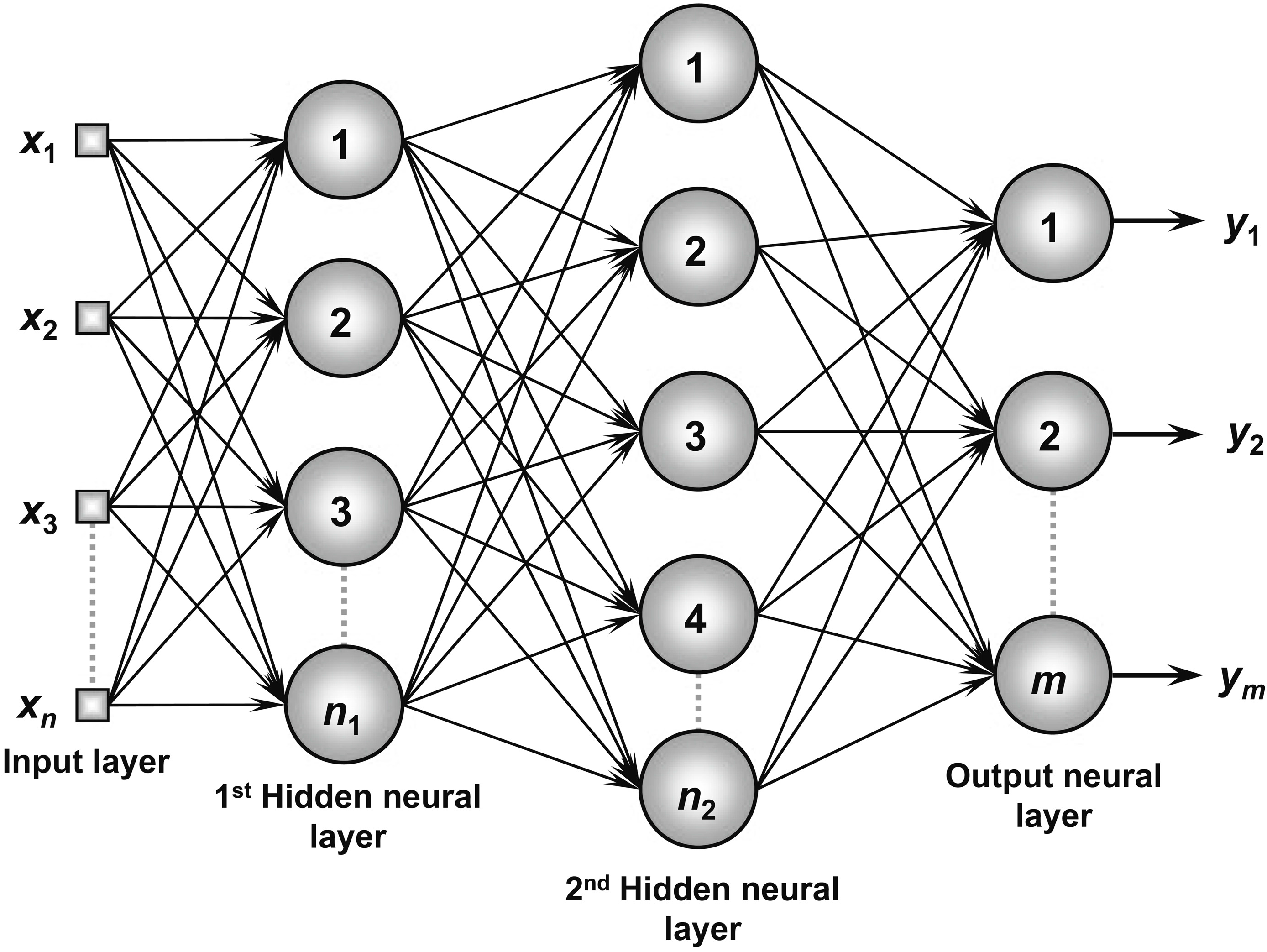
3. An Artificial Neural Network
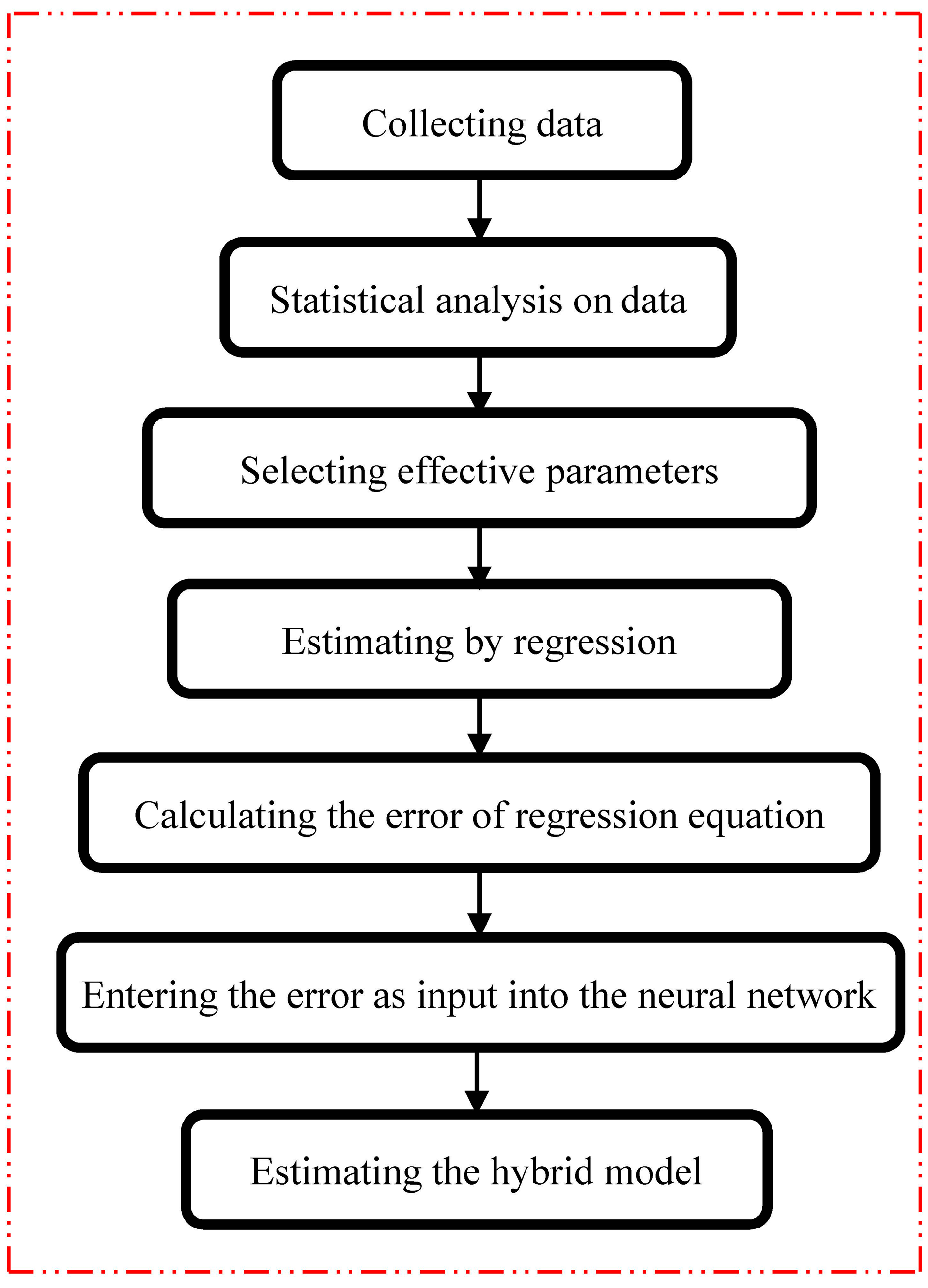
4. The Hybrid Methodology
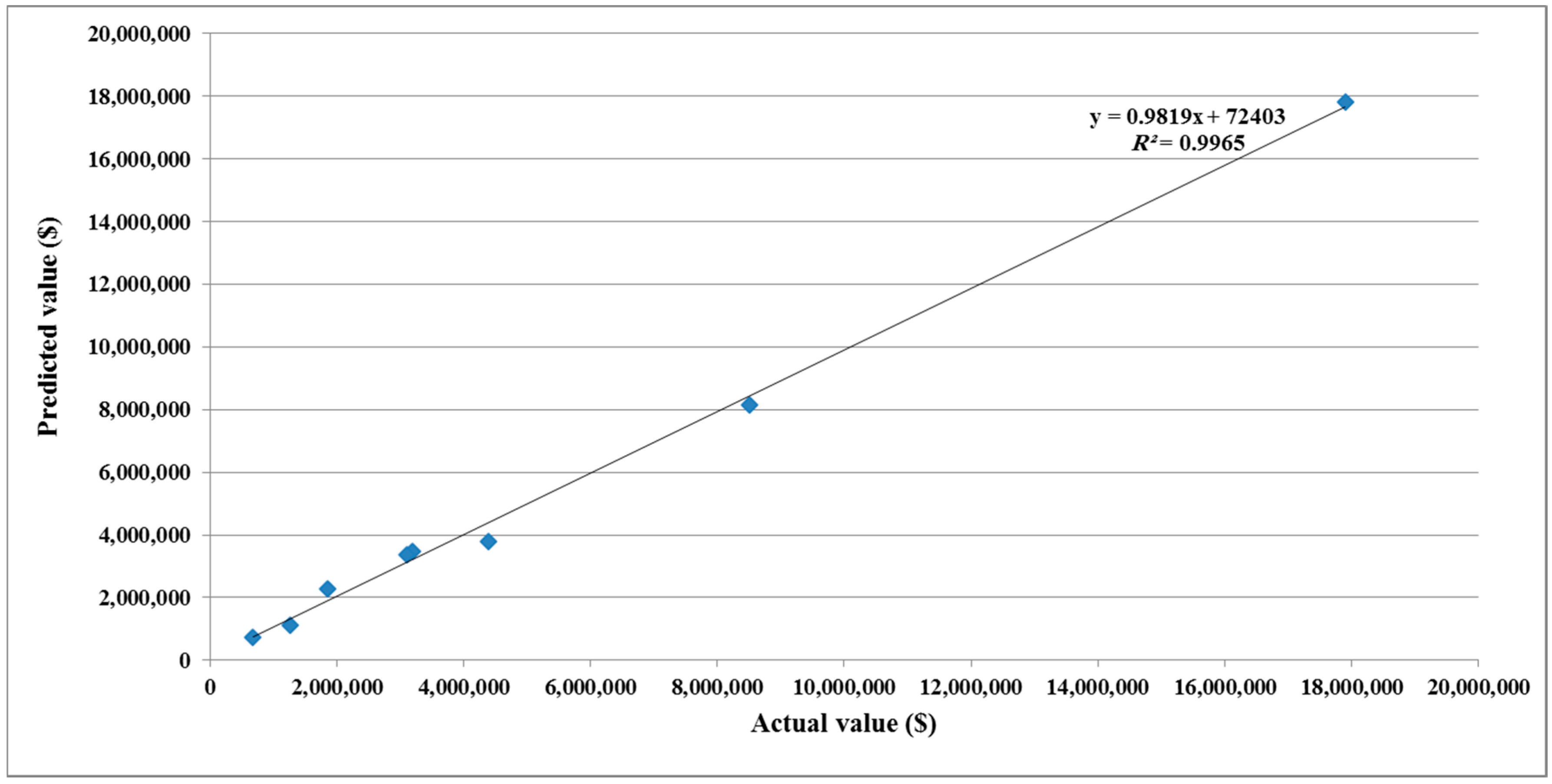
5. Model Performance
6. The Data
7. The Implementation of the Proposed Model
8. The Comparison of the Developed Model with Other Models
9. Sensitivity Analysis
10. Conclusions
Author Contributions
Conflicts of Interest
References
- Devi, L.P.; Palaniappan, S. A study on energy use for excavation and transport of soil during building construction. J. Clean. Prod. 2017, 164, 543–556. [Google Scholar] [CrossRef]
- Atkinson, T. Selection and sizing of excavating equipment. In SME Mining Engineering Handbook; Society for Mining, Metallurgy, and Exploration: Littleton, CO, USA, 1992; pp. 1311–1333. [Google Scholar]
- Tatiya, R.R. Surface and Underground Excavations—Methods, Techniques and Equipment; Taylor & Francis Group plc: London, UK, 2005. [Google Scholar]
- Huang, J.; Dong, Z.; Quan, L.; Jin, Z.; Lan, Y.; Wang, Y. Development of a dual displacement controlled circuit for hydraulic shovel swing motion. Autom. Constr. 2015, 57, 166–174. [Google Scholar] [CrossRef]
- Elevli, S.; Elevli, B. Performance measurement of mining equipments by utilizing OEE. Acta Montan. Slovaca 2010, 15, 95–101. [Google Scholar]
- Lashgari, A.; Yazdani-Chamzini, A.; Fouladgar, M.M.; Zavadskas, E.K.; Shafiee, S.; Abbate, N. Equipment selection using fuzzy multi criteria decision making model: Key study of Gole Gohar iron mine. Inz. Econ. 2012, 23, 125–136. [Google Scholar] [CrossRef]
- Sayadi, A.R.; Lashgari, A.; Fouladgar, M.M.; Skibniewski, M. Estimating capital and operational costs of backhoe shovels. J. Civ. Eng. Manag. 2012, 18, 378–385. [Google Scholar] [CrossRef]
- Mutmansky, J.M.; Suboleski, S.C.; O’Hara, T.A.; Prasad, K.V.K. Cost comparisons. In SME Mining Engineering Handbook, 2nd ed.; Hartman, H.L., Ed.; Society for Mining, Metallurgy, and Exploration: Littleton, CO, USA, 1992; pp. 2070–2089. [Google Scholar]
- Anon. Estimating Preproduction and Operating Costs of Small Underground Deposits (CANMET); Canadian Government Publishing Centre: Ottawa, ON, Canada, 1986.
- Mular, A.L.; Poulin, R. CAPCOSTS: A Handbook for Estimating Mining and Mineral Processing Equipment Costs and Capital Expenditures and Aiding Mineral Project Evaluations; CIM Bulletin Special, 47; Canadian Institute of Mining and Metallurgy: Montréal, QC, Canada, 1998. [Google Scholar]
- Mular, A.L. Mining and Mineral Processing Equipment Costs and Preliminary Capital Cost Estimation; CIM Bulletin Special, 25; Canadian Institute of Mining and Metallurgy: Montreal, QC, Canada, 1982. [Google Scholar]
- Lanz, T.; Noakes, M. Cost Estimation Handbook for the Australian Mining Industry; Australasian Institute of Mining and Metallurgy (Aus IMM): Carlton South, Australia, 1993. [Google Scholar]
- USBM. US Bureau of Mines Cost Estimating System Handbook, Mining and Beneficiation of Metallic and Nonmetallic Minerals Expected Fossil Fuels in the United States and Canada; United States Bureau of Mines: Denver, CO, USA, 1987; pp. 10–87.
- Mohutsiwa, M.; Musingwini, C. Parametric estimation of capital costs for establishing a coal mine: South Africa case study. J. South. Afr. Inst. Min. Metall. 2015, 115, 789–797. [Google Scholar] [CrossRef]
- Sayadi, A.R.; Lashgari, A.; Paraszczak, J. Hard-rock LHD cost estimation using single and multiple regressions based on principal component analysis. Tunn. Undergr. Space Technol. 2012, 27, 133–141. [Google Scholar] [CrossRef]
- O’Hara, T.A. Quick guide to the evaluation of ore bodies. CIM Bull. 1998, 88, 34–43. [Google Scholar]
- O’Hara, T.A. Mine Evaluation, Mineral Industry Costs; Hoskins, J.R., Ed.; Northwest Mining Association: Spokane, WA, USA, 1982; pp. 89–99. [Google Scholar]
- O’Hara, T.A. Quick Guide to Mine Operating Costs and Revenue; Paper No. 186; CIM Annual General Meeting: Toronto, ON, Canada, 1987. [Google Scholar]
- O’Hara, T.A.; Suboleski, C.S. Costs and Cost Estimation. In SME Mining Engineering Handbook; Society for Mining, Metallurgy, and Exploration: Littleton, CO, USA, 1992; Volume 1, pp. 405–424. [Google Scholar]
- Camm, T.W. Simplified cost models for pre-feasibility mineral evaluations. Min. Eng. 1994, 46, 559–562. [Google Scholar]
- Rudenno, V. The Mining Valuation Handbook: Australian Mining and Energy Valuation for Investors and Management; Australian Print Group: Victoria, Australia, 1998. [Google Scholar]
- Sayadi, A.R.; Khademi, J.; Rahimi, M.A. Estimating the energy costs of mine equipment using an information system. In Proceedings of the 24th International Mining Congress and Exhibition of Turkey, Antalya, Turkey, 14–17 April 2015; pp. 9–18. [Google Scholar]
- Wei, Y.; Qiu, J.; Shi, P.; Chadli, M. Fixed-order piecewise-affine output feedback controller for fuzzy-affine-model-based nonlinear systems with time-varying delay. IEEE Trans. Circuits Syst. I Regul. Pap. 2017, 64, 945–958. [Google Scholar] [CrossRef]
- Wei, Y.; Qiu, J.; Karimi, H.R. Fuzzy-affine-model-based memory filter design of nonlinear systems with time-varying delay. IEEE Trans. Fuzzy Syst. 2017, PP, 1. [Google Scholar] [CrossRef]
- Singh, V.; Gupta, I.; Gupta, H.O. ANN-based estimator for distillation using Levenberg-Marquardt approach. Eng. Appl. Artif. Intell. 2007, 20, 249–259. [Google Scholar] [CrossRef]
- Yamamura, S. Clinical application of artificial neural network (ANN) modeling to predict pharmacokinetic parameters of severely ill patients. Adv. Drug Deliv. Rev. 2003, 55, 1233–1251. [Google Scholar] [CrossRef]
- Lian-Guo, W.; Zhi-Kang, Z.; Yin-Long, L.; Hong-Bo, Y.; Sheng-Qiang, Y.; Jian, S.; Jin-Yao, Z. Combined ANN prediction model for failure depth of coal seam floors. Min. Sci. Technol. 2009, 19, 684–688. [Google Scholar]
- Fast, M.; Assadi, M.; De, S. Development and multi-utility of an ANN model for an industrial gas turbine. Appl. Energy 2009, 86, 9–17. [Google Scholar] [CrossRef]
- Lee, J.; Sanmugarasa, K.; Blumenstein, M.; Loo, Y.C. Improving the reliability of a Bridge Management System (BMS) using an ANN-based Backward Prediction Model (BPM). Autom. Constr. 2008, 17, 758–772. [Google Scholar] [CrossRef]
- Jalali-Heravi, M.; Asadollahi-Baboli, M.; Mani-Varnosfaderani, A. Shuffling multivariate adaptive regression splines and adaptive neuro-fuzzy inference system as tools for QSAR study of SARS inhibitors. J. Pharm. Biomed. Anal. 2009, 50, 853–860. [Google Scholar] [CrossRef] [PubMed]
- Verlinden, B.; Duflou, J.R.; Collin, P.; Cattrysse, D. Cost estimation for sheet metal parts using multiple regression and artificial neural networks: A case study. Int. J. Prod. Econ. 2008, 111, 484–492. [Google Scholar] [CrossRef]
- Mesroghli, S.; Jorjani, E.; Chelgani, S.C. Estimation of gross calorific value based on coal analysis using regression and artificial neural networks. Int. J. Coal Geol. 2009, 79, 49–54. [Google Scholar] [CrossRef]
- Sahoo, G.B.; Schladow, S.G.; Reuter, J.E. Forecasting stream water temperature using regression analysis, artificial neural network, and chaotic non-linear dynamic models. J. Hydrol. 2009, 378, 325–342. [Google Scholar] [CrossRef]
- Gu, Y.; Wu, L.; Tang, S. A fuzzy neutral-network-driven weighting system for electric shovel. In Advances in Neural Networks—ISNN 2008; Sun, F., Zhang, J., Tan, Y., Cao, J., Yu, W., Eds.; Lecture Notes in Computer Science; Springer: Berlin/Heidelberg, Germany, 2008; Volume 5264, pp. 526–532. [Google Scholar]
- Guo, J.; Zhao, X.; Guo, J.; Yuan, X.; Dong, S.; Xiong, Z. Model updating of suspended-dome using artificial neural networks. Adv. Struct. Eng. 2017, 20, 1727–1743. [Google Scholar] [CrossRef]
- Du, Y.; Chen, Z.; Zhang, C.; Cao, X. Research on axial bearing capacity of rectangular concrete-filled steel tubular columns based on artificial neural networks. Front. Comput. Sci. 2017, 11, 863–873. [Google Scholar] [CrossRef]
- Gardner, B.J.; Gransberg, D.D.; Rueda, J.A. Stochastic conceptual cost estimating of highway projects to communicate uncertainty using bootstrap sampling. ASCE-ASME J. Risk Uncertain. Eng. Part A Civ. Eng. 2017, 3. [Google Scholar] [CrossRef]
- El-Gohary, K.M.; Aziz, R.F.; Abdel-Khalek, H.A. Engineering approach using ANN to improve and predict construction labor productivity under different influences. J. Constr. Eng. Manag. 2017, 143. [Google Scholar] [CrossRef]
- Cao, M.S.; Pan, L.X.; Gao, Y.F.; Novak, D.; Ding, Z.C.; Lehky, D.; Li, X.L. Neural network ensemble-based parameter sensitivity analysis in civil engineering systems. Neural Comput. Appl. 2017, 28, 1583–1590. [Google Scholar] [CrossRef]
- Abdeljaber, O.; Avci, O.; Kiranyaz, S.; Gabbouj, M.; Inman, D.J. Real-time vibration-based structural damage detection using one-dimensional convolutional neural networks. J. Sound Vib. 2017, 388, 154–170. [Google Scholar] [CrossRef]
- Benali, A.; Boukhatem, B.; Hussien, M.N.; Nechnech, A.; Karray, M. Prediction of axial capacity of piles driven in non-cohesive soils based on neural networks approach. J. Civ. Eng. Manag. 2017, 23, 393–408. [Google Scholar] [CrossRef]
- Yousefi, V.; Yakhchali, S.H.; Khanzadi, M.; Mehrabanfar, E.; Šaparauskas, J. Proposing a neural network model to predict time and cost claims in construction projects. J. Civ. Eng. Manag. 2016, 22, 967–978. [Google Scholar] [CrossRef]
- Ustinovichius, L.; Peckienė, A.; Popov, V. A model for spatial planning of site and building using BIM methodology. J. Civ. Eng. Manag. 2017, 23, 173–182. [Google Scholar] [CrossRef]
- Wang, W.C.; Bilozerov, T.; Dzeng, R.J.; Hsiao, F.Y.; Wang, K.C. Conceptual cost estimations using neuro-fuzzy and multi-factor evaluation methods for building projects. J. Civ. Eng. Manag. 2017, 23, 1–14. [Google Scholar] [CrossRef]
- Monjezi, M.; Rezaei, M.; Varjani, A.Y. Prediction of rock fragmentation due to blasting in Gol-E-Gohar iron mine using fuzzy logic. Int. J. Rock Mech. Min. Sci. 2009, 46, 1273–1280. [Google Scholar] [CrossRef]
- Bourquin, J.; Schmidli, H.; Hoogevest, P.; Leuenberger, H. Advantages of Artificial Neural Networks (ANNs) as alternative modelling technique for data sets showing non-linear relationships using data from a galenical study on a solid dosage form. Eur. J. Pharm. Sci. 1998, 7, 5–16. [Google Scholar] [CrossRef]
- Malinowski, P.; Ziembicki, P. Analysis of district heating network monitoring by neural networks classification. J. Civ. Eng. Manag. 2006, 12, 21–28. [Google Scholar]
- He, X.; Xu, S. Process Neural Networks Theory and Applications; Springer: Berlin/Heidelberg, Germany, 2007. [Google Scholar]
- Engelbrecht, A.P. Computational Intelligence: An Introduction; John Wiley & Sons, Ltd.: Hoboken, NJ, USA, 2002. [Google Scholar]
- Sumathi, S.; Paneerselvam, S. Computational Intelligence Paradigms: Theory & Applications Using MATLAB; Taylor and Francis Group, LLC: Oxford, UK, 2010. [Google Scholar]
- Khashei, M.; Bijari, M. A novel hybridization of artificial neural networks and ARIMA models for time series forecasting. Appl. Soft Comput. 2011, 11, 2664–2675. [Google Scholar] [CrossRef]
- Zhang, G.P. Time series forecasting using a hybrid ARIMA and neural network model. Neurocomputing 2003, 50, 159–175. [Google Scholar] [CrossRef]
- Farid, M.; Hossein Abadi, M.M.; Yazdani-Chamzini, A.; Yakhchali, S.H.; Basiri, M.H. Developing a new model based on neuro-fuzzy system for predicting roof fall in coal mines. Neural Comput. Appl. 2013, 23, 129–137. [Google Scholar] [CrossRef]
- Nash, J.E.; Sutcliffe, J.V. River flow forecasting through conceptual models, I. A discussion of principles. J. Hydrol. 1970, 10, 282–290. [Google Scholar] [CrossRef]
- Razani, M.; Yazdani-Chamzini, A.; Yakhchali, S.H. A novel fuzzy inference system for predicting roof fall rate in underground coal mines. Saf. Sci. 2013, 55, 26–33. [Google Scholar] [CrossRef]
- Yazdani-Chamzini, A.; Yakhchali, S.H.; Volungevičienė, D.; Zavadskas, E.K. Forecasting gold price changes by using adaptive network fuzzy inference system. J. Bus. Econ. Manag. 2012, 13, 994–1010. [Google Scholar] [CrossRef]
- Info Mine: Mining Cost Service Indexes. Available online: http://www.infomine.com (accessed on 26 June 2015).
- Wang, W.; Van Gelder, P.H.A.J.M.; Vrijling, J.K.; Ma, J. Forecasting daily streamflow using hybrid ANN models. J. Hydrol. 2006, 324, 383–399. [Google Scholar] [CrossRef]
- Srinivas, Y.; Raj, A.S.; Oliver, D.H.; Muthuraj, D.; Chandrasekar, N. A robust behavior of Feed forward back propagation algorithm of Artificial Neural Networks in the application of vertical electrical sounding data inversion. Geosci. Front. 2012, 3, 729–736. [Google Scholar] [CrossRef]
- Basheer, I.A.; Hajmeer, M. Artificial neural networks: Fundamentals, computing, design, and application. J. Microbiol. Methods 2000, 43, 3–31. [Google Scholar] [CrossRef]
- Wei, Y.; Qiu, J.; Karimi, H.R.; Ji, W. A novel memory filtering design for semi-Markovian jump time-delay systems. IEEE Trans. Syst. Man Cybern. 2017, PP, 1–13. [Google Scholar] [CrossRef]
- Qiu, J.; Wei, Y.; Karimi, H.R.; Gao, H. Reliable Control of Discrete-Time Piecewise-Affine Time-Delay Systems via Output Feedback. IEEE Trans. Reliab. 2017, 57, 1491–1550. [Google Scholar] [CrossRef]
- Ross, T.J. Fuzzy Logic with Engineering Applications, 3rd ed.; John Wiley & Sons Ltd.: Hoboken, NJ, USA, 2010. [Google Scholar]
- Yazdani-Chamzini, A.; Razani, M.; Yakhchali, S.H.; Zavadskas, E.K.; Turskis, Z. Developing a fuzzy model based on subtractive clustering for road header performance prediction. Autom. Constr. 2013, 35, 111–120. [Google Scholar] [CrossRef]


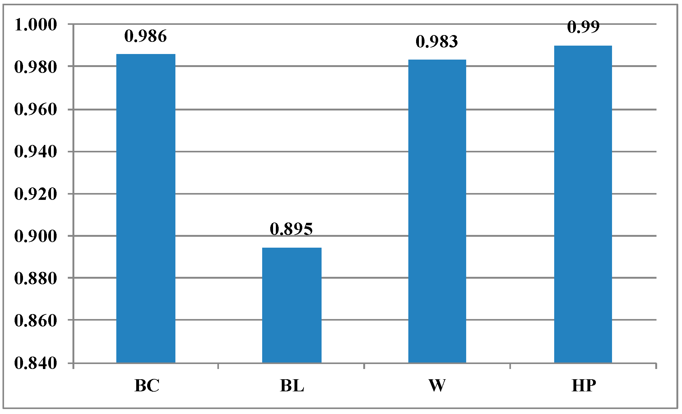
| Machine Type | Operator | Bucket Capacity (BC) | Boom Length (BL) | Weight (W) | Horsepower (HP) | Capital Cost (CC) |
|---|---|---|---|---|---|---|
| Cable | Min | 7 | 35 | 556,000 | 685 | 2,800,000 |
| Max | 80 | 64 | 4,500,000 | 7000 | 17,900,000 | |
| Mean | 31.29 | 50.57 | 1,517,071 | 2923.85 | 7,871,429 | |
| Standard deviation | 21.27 | 9.04 | 1,084,127.97 | 1989.71 | 4,443,392.42 | |
| Hydraulic | Min | 3 | 15.4 | 95,900 | 250 | 605,000 |
| Max | 44 | 39.3 | 1,399,000 | 3000 | 6,900,000 | |
| Mean | 12.74 | 28.74 | 385,318.8 | 873.56 | 2,068,313 | |
| Standard deviation | 9.97 | 6.96 | 334,189.25 | 700.14 | 1,781,125.17 |
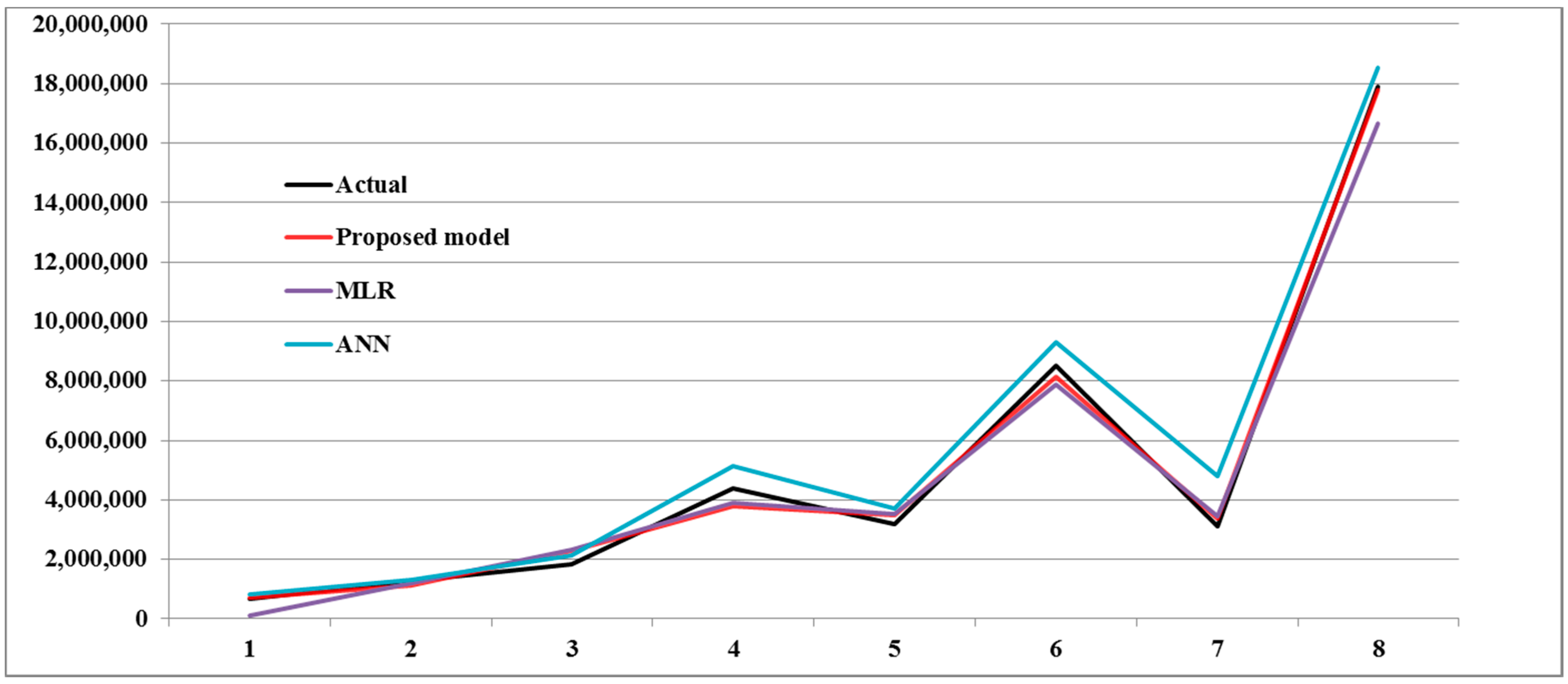
| Case | Actual | MVR | ANN | Proposed Model |
|---|---|---|---|---|
| 1 | 680,000 | 120,755.6 | 815,732.3 | 716,660.3 |
| 2 | 1,263,000 | 120,2621 | 1,299,821 | 1,115,828 |
| 3 | 1,850,000 | 2,338,051 | 2,145,405 | 2,293,947 |
| 4 | 4,400,000 | 3,903,419 | 5,124,051 | 3,802,985 |
| 5 | 3,200,000 | 3,528,523 | 3,719,688 | 3,470,780 |
| 6 | 8,500,000 | 7,865,014 | 9,298,305 | 8,150,003 |
| 7 | 3,100,000 | 3,431,278 | 4,803,671 | 3,378,503 |
| 8 | 17,900,000 | 16,661,424 | 18,551,802 | 17,801,455 |
| Model | R2 | NMSE | MAPE |
|---|---|---|---|
| Proposed model | 0.9965 | 0.0035 | 9.59% |
| ANN | 0.9924 | 0.0076 | 17.44% |
| MVR | 0.9941 | 0.0059 | 20% |
© 2017 by the authors. Licensee MDPI, Basel, Switzerland. This article is an open access article distributed under the terms and conditions of the Creative Commons Attribution (CC BY) license (http://creativecommons.org/licenses/by/4.0/).
Share and Cite
Yazdani-Chamzini, A.; Zavadskas, E.K.; Antucheviciene, J.; Bausys, R. A Model for Shovel Capital Cost Estimation, Using a Hybrid Model of Multivariate Regression and Neural Networks. Symmetry 2017, 9, 298. https://doi.org/10.3390/sym9120298
Yazdani-Chamzini A, Zavadskas EK, Antucheviciene J, Bausys R. A Model for Shovel Capital Cost Estimation, Using a Hybrid Model of Multivariate Regression and Neural Networks. Symmetry. 2017; 9(12):298. https://doi.org/10.3390/sym9120298
Chicago/Turabian StyleYazdani-Chamzini, Abdolreza, Edmundas Kazimieras Zavadskas, Jurgita Antucheviciene, and Romualdas Bausys. 2017. "A Model for Shovel Capital Cost Estimation, Using a Hybrid Model of Multivariate Regression and Neural Networks" Symmetry 9, no. 12: 298. https://doi.org/10.3390/sym9120298
APA StyleYazdani-Chamzini, A., Zavadskas, E. K., Antucheviciene, J., & Bausys, R. (2017). A Model for Shovel Capital Cost Estimation, Using a Hybrid Model of Multivariate Regression and Neural Networks. Symmetry, 9(12), 298. https://doi.org/10.3390/sym9120298