
Multiple Signal Classification Algorithm Based Electric Dipole Source Localization Method in an Underwater Environment


Abstract
:1. Introduction
2. Localization of Electric Dipole Source in Finite Region
2.1. Localization Model of Electric Dipole Source
2.2. Localization Based on the Multiple Signal Classification Algorithm
- Step 1: Discretize the boundary of the locating area and calculate the boundary matrix according to the prior information about the boundary. By inverting the boundary matrix, we have .
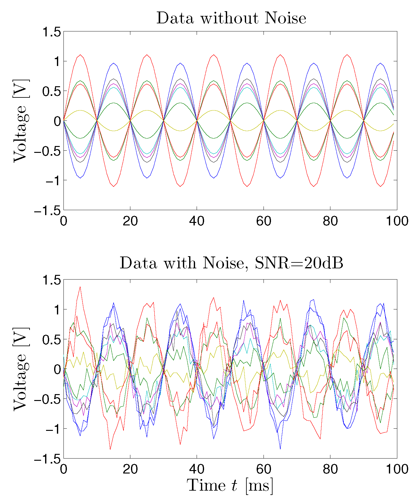
- Step 2: By measuring the voltage of each channel of the receiving antenna array, the matrix is formed with the size of .
- Step 3: According to (23), the covariance matrix can be constructed.
- Step 4: Obtain the required signal subspace and noise subspace via the eigendecomposition of the constructed matrix .
- Step 5: Mesh the locating area with a set of spatial points .
- Step 6: Calculate the matrix according to (17) with the estimated dipole source position , .
- Step 7: Obtain the eigenvalues , and via the generalized eigendecomposition , where .
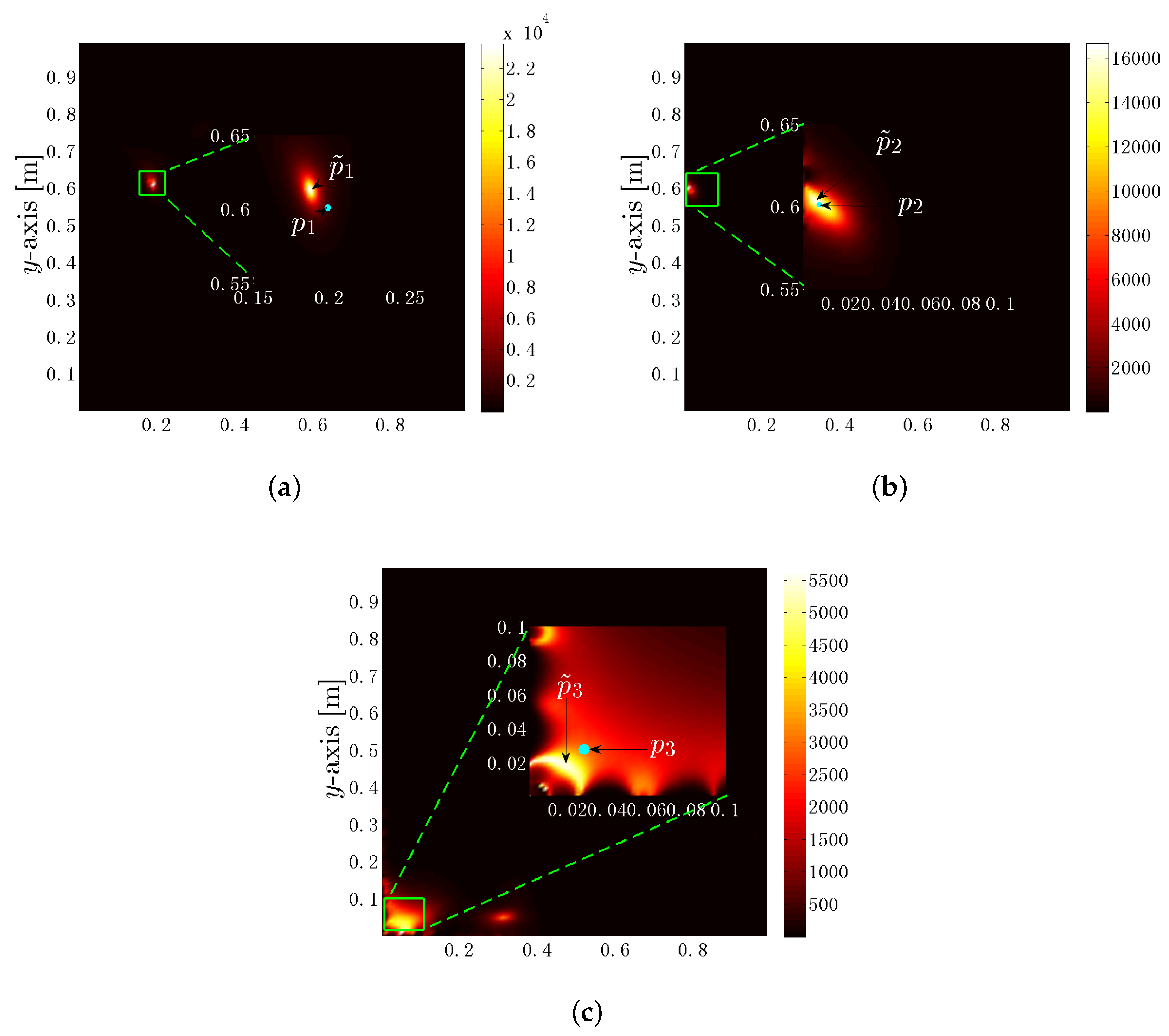
- Step 8: Find the global minima of . The dipole source position is estimated by .
- Step 1: Scan the entire locating region with the interval of by the use of point-by-point scan method, and output the estimation position .
- Step 2: Scan the local region near the estimation position with the interval of , where .
- Step 3: If m equals to M, go to Step 4. Otherwise, update the estimation position , update the interval by , reduce the searching range and go to Step 2.
- Step 4: Estimate the position by using the CG method and output the final estimation position.
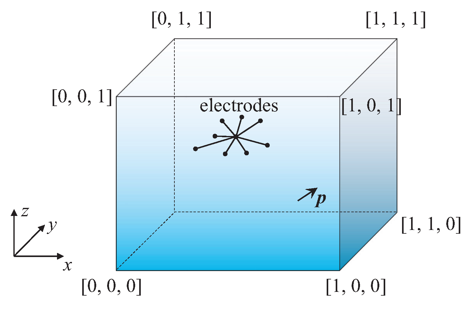
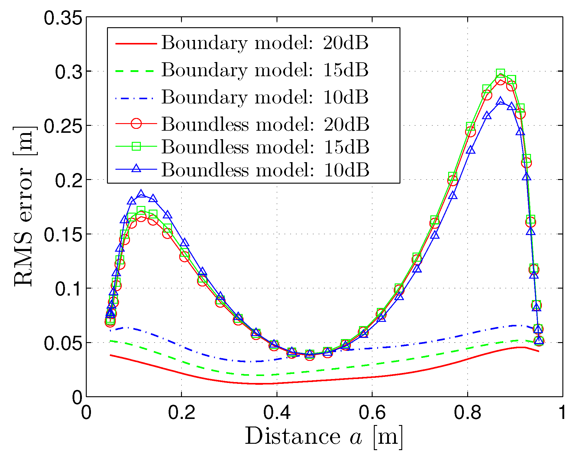
3. Numerical Examples
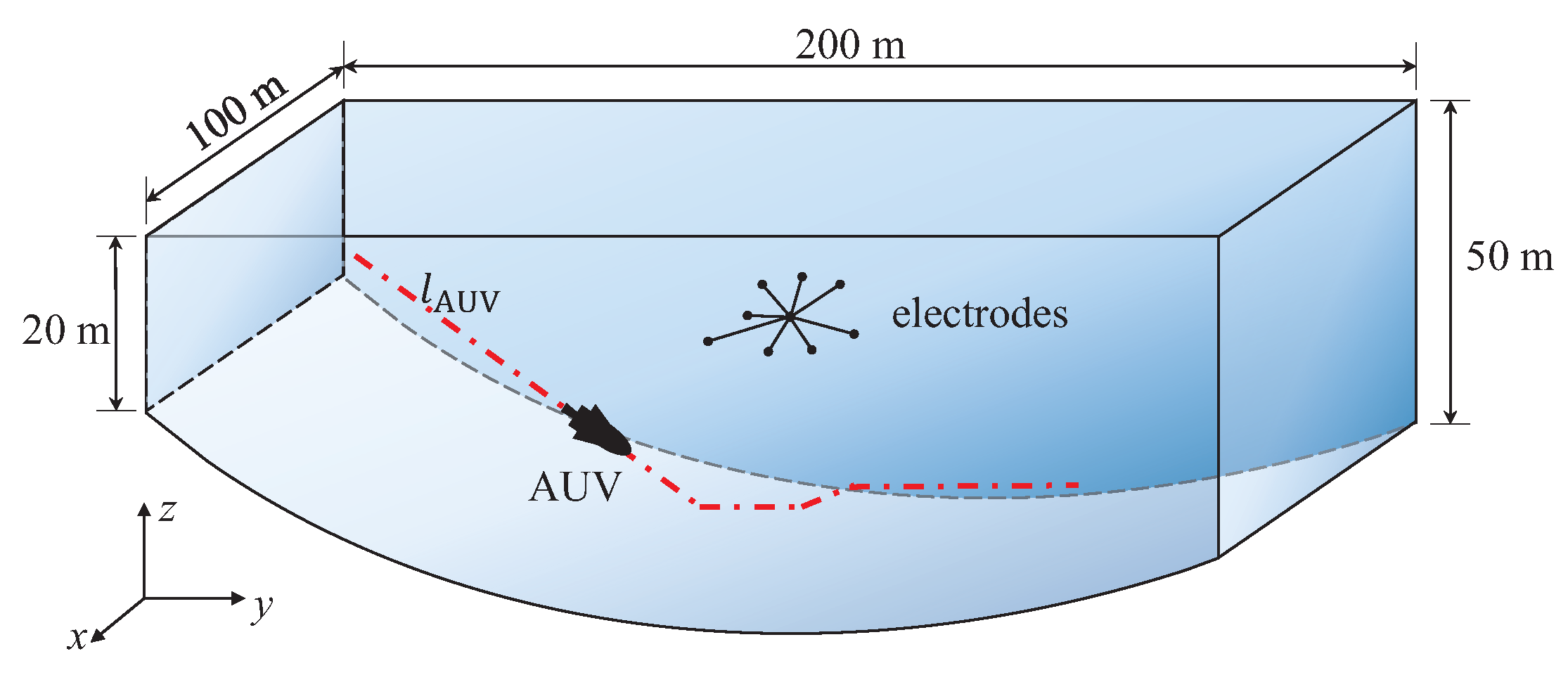
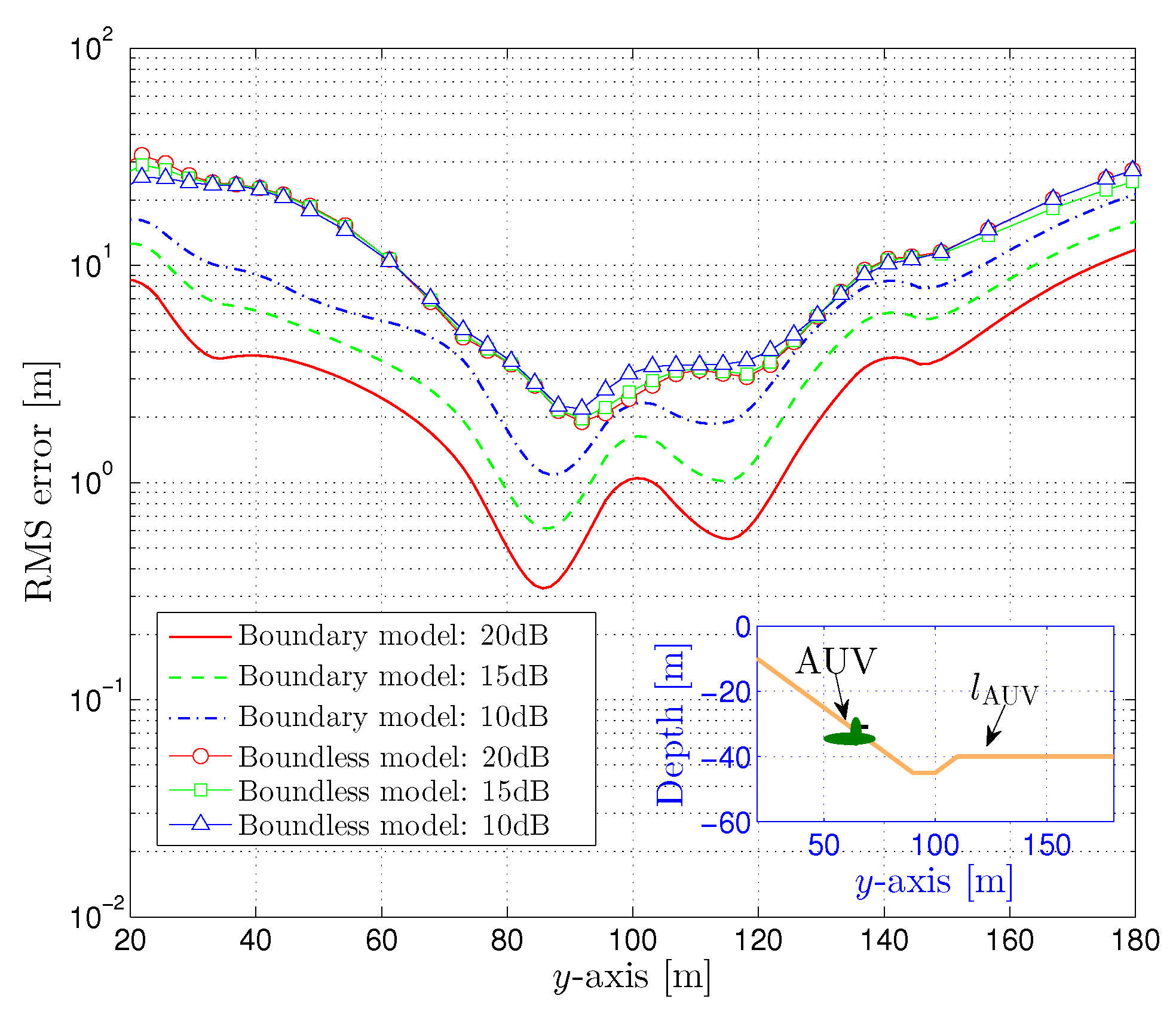
4. Experiment
5. Conclusions
Acknowledgments
Author Contributions
Conflicts of Interest
References
- Carroll, P.; Zhou, S.; Zhou, H.; Xu, X.; Cui, J.H.; Willett, P. Underwater Localization and Tracking of Physical Systems. J. Electr. Comput. Eng. 2012, 2012, 2. [Google Scholar] [CrossRef]
- Lefort, R.; Real, G.; Drémeau, A. Direct regressions for underwater acoustic source localization in fluctuating oceans. Appl. Acoust. 2017, 116, 303–310. [Google Scholar] [CrossRef]
- Li, B.; Zhou, S.; Stojanovic, M.; Freitag, L.; Willett, P. Multicarrier Communication over Underwater Acoustic Channels with Nonuniform Doppler Shifts. IEEE J. Ocean. Eng. 2008, 33, 198–209. [Google Scholar]
- Esmaiel, H.; Jiang, D. Review Article: Multicarrier Communication for Underwater Acoustic Channel. Int. J. Commun. Netw. Syst. Sci. 2013, 6, 361–376. [Google Scholar] [CrossRef]
- Rango, F.D.; Veltri, F.; Fazio, P. A multipath fading channel model for underwater shallow acoustic communications. In Proceedings of the IEEE International Conference on Communications (ICC), Ottawa, ON, Canada, 10–15 June 2012; pp. 3811–3815. [Google Scholar]
- Park, D.; Kwak, K.; Kim, J.; Wan, K.C. Underwater sensor network using received signal strength of electromagnetic waves. In Proceedings of the IEEE/RSJ International Conference on Intelligent Robots and Systems (IROS), Hamburg, Germany, 28 September–2 October 2015; pp. 1052–1057. [Google Scholar]
- Quintanadíaz, G.; Menarodríguez, P.; Pérezálvarez, I.; Jiménez, E.; Dortanaranjo, B.P.; Zazo, S.; Pérez, M.; Quevedo, E.; Cardona, L.; Hernández, J. Underwater Electromagnetic Sensor Networks—Part I: Link Characterization. Sensors 2017, 17, 189. [Google Scholar] [CrossRef] [PubMed]
- Soderberg, E.F. ELF noise in the sea at depths from 30 to 300 meters. J. Geophys. Res. 1969, 74, 2376–2387. [Google Scholar] [CrossRef]
- Zazo, J.; Macua, S.V.; Zazo, S.; Pérez, M.; Pérez-Álvarez, I.; Jiménez, E.; Cardona, L.; Brito, J.H.; Quevedo, E. Underwater Electromagnetic Sensor Networks, Part II: Localization and Network Simulations. Sensors 2016, 16, 2176. [Google Scholar] [CrossRef] [PubMed]
- Duecker, D.A.; Geist, A.R.; Hengeler, M.; Kreuzer, E.; Pick, M.A.; Rausch, V.; Solowjow, E. Embedded Spherical Localization for Micro Underwater Vehicles Based on Attenuation of Electro-Magnetic Carrier Signals. Sensors 2017, 17, 959. [Google Scholar] [CrossRef] [PubMed]
- Lebastard, V.; Chevallereau, C.; Amrouche, A.; Jawad, B.; Girin, A.; Boyer, F.; Gossiaux, P.B. Underwater robot navigation around a sphere using electrolocation sense and Kalman filter. In Proceedings of the IEEE/RSJ International Conference on Intelligent Robots and Systems, Taipei, Taiwan, 18–22 October 2010; pp. 4225–4230. [Google Scholar]
- Boyer, F.; Lebastard, V.; Chevallereau, C.; Servagent, N. Underwater Reflex Navigation in Confined Environment Based on Electric Sense. IEEE Trans. Robot. 2013, 29, 945–956. [Google Scholar] [CrossRef]
- Mosher, J.C.; Leahy, R.M. EEG and MEG source localization using recursively applied (RAP) MUSIC. In Proceedings of the Conference Record of The Thirtieth Asilomar Conference on Signals, Systems and Computers, Pacific Grove, CA, USA, 3–6 November 1996; pp. 1201–1207. [Google Scholar]
- Mosher, J.C.; Leahy, R.M.; Lewis, P.S. EEG and MEG: Forward solutions for inverse methods. IEEE Trans. Bio-Med. Eng. 1999, 46, 245–259. [Google Scholar] [CrossRef]
- Hong, J.H.; Ahn, M.; Kim, K.; Jun, S.C. Localization of coherent sources by simultaneous MEG and EEG beamformer. Med. Biol. Eng. Comput. 2013, 51, 1121–1135. [Google Scholar] [CrossRef] [PubMed]
- Shahbazi, F.; Ewald, A.; Nolte, G. Self-Consistent MUSIC: An approach to the localization of true brain interactions from EEG/MEG data. Neuroimage 2015, 112, 299. [Google Scholar] [CrossRef] [PubMed]
- Shahbazi, F.; Ziehe, A.; Nolte, G. Self-Consistent MUSIC algorithm to localize multiple sources in acoustic imaging. In Proceedings of the 4th Berlin Beamforming Conference, Berlin, Germany, 22–23 February 2012. [Google Scholar]
- Heller, L.; Hulsteyn, D.B.V. Brain stimulation using electromagnetic sources: Theoretical aspects. Biophys. J. 1992, 63, 129–138. [Google Scholar] [CrossRef]
- Katsikadelis, J. Boundary Elements. Theory and Applications; Elsevier Science: Oxford, UK, 2002. [Google Scholar]
- Mosher, J.C.; Leahy, R.M. Recursive MUSIC: A framework for EEG and MEG source localization. IEEE Trans. Biomed. Eng. 1998, 45, 1342–1354. [Google Scholar] [CrossRef] [PubMed]
- Sekihara, K.; Poeppel, D.; Marantz, A.; Koizumi, H.; Miyashita, Y. Noise covariance incorporated MEG-MUSIC algorithm: A method for multiple-dipole estimation tolerant of the influence of background brain activity. IEEE Trans. Biomed. Eng. 1997, 44, 839–847. [Google Scholar] [CrossRef] [PubMed]
- Mosher, J.C.; Leahy, R.M. Source localization using recursively applied and projected (RAP) MUSIC. IEEE Trans. Signal Process. 1999, 47, 332–340. [Google Scholar] [CrossRef]


| Electrode Index | 1 | 2 | 3 | 4 | 5 | 6 | 7 | 8 | 9 |
|---|---|---|---|---|---|---|---|---|---|
| x (m) | 0.4 | 0.5 | 0.6 | 0.4 | 0.5 | 0.7 | 0.6 | 0.34 | 0.5 |
| y (m) | 0.6 | 0.4 | 0.6 | 0.4 | 0.5 | 0.3 | 0.5 | 0.55 | 0.5 |
| z (m) | 0.5 | 0.6 | 0.6 | 0.4 | 0.7 | 0.6 | 0.4 | 0.55 | 0.5 |
| Electrode Index | 1 | 2 | 3 | 4 | 5 | 6 | 7 | 8 | 9 |
|---|---|---|---|---|---|---|---|---|---|
| x (m) | 40 | 50 | 50 | 50 | 40 | 60 | 50 | 50 | 50 |
| y (m) | 80 | 140 | 100 | 100 | 100 | 100 | 80 | 120 | 100 |
| z (m) | −30 | −30 | −40 | −20 | −30 | −30 | −30 | −30 | −30 |
| Electrode Index | 1 | 2 | 3 | 4 | 5 | 6 | 7 | 8 | 9 |
|---|---|---|---|---|---|---|---|---|---|
| x (m) | −0.099 | 0 | 0.099 | 0.14 | 0.099 | 0 | 0 | ||
| y (m) | 0.099 | 0.14 | 0.099 | 0 | 0 | 0 | |||
| z (m) | −0.3 | −0.3 | −0.3 | −0.3 |
| Dipole Source | Actual Position | Estimated Position | Maximum Error (m) | Minimum Error (m) | RMS Error (m) |
|---|---|---|---|---|---|
| 0.035 | 0.024 | 0.026 | |||
| 0.009 | 0.009 | 0.009 | |||
| 0.076 | 0.023 | 0.046 | |||
| 0.026 | 0.017 | 0.020 | |||
| 0.033 | 0.028 | 0.030 |
© 2017 by the authors. Licensee MDPI, Basel, Switzerland. This article is an open access article distributed under the terms and conditions of the Creative Commons Attribution (CC BY) license (http://creativecommons.org/licenses/by/4.0/).
Share and Cite
Xu, Y.; Xue, W.; Li, Y.; Guo, L.; Shang, W. Multiple Signal Classification Algorithm Based Electric Dipole Source Localization Method in an Underwater Environment. Symmetry 2017, 9, 231. https://doi.org/10.3390/sym9100231
Xu Y, Xue W, Li Y, Guo L, Shang W. Multiple Signal Classification Algorithm Based Electric Dipole Source Localization Method in an Underwater Environment. Symmetry. 2017; 9(10):231. https://doi.org/10.3390/sym9100231
Chicago/Turabian StyleXu, Yidong, Wei Xue, Yingsong Li, Lili Guo, and Wenjing Shang. 2017. "Multiple Signal Classification Algorithm Based Electric Dipole Source Localization Method in an Underwater Environment" Symmetry 9, no. 10: 231. https://doi.org/10.3390/sym9100231
APA StyleXu, Y., Xue, W., Li, Y., Guo, L., & Shang, W. (2017). Multiple Signal Classification Algorithm Based Electric Dipole Source Localization Method in an Underwater Environment. Symmetry, 9(10), 231. https://doi.org/10.3390/sym9100231