Skein Invariants of Links and Their State Sum Models

Abstract

We present the new skein invariants of classical links, $H\left[H\right]$, $K\left[K\right]$ and $D\left[D\right]$, based on the invariants of links, H, K and D, denoting the regular isotopy version of the Homflypt polynomial, the Kauffman polynomial and the Dubrovnik polynomial. The invariants are obtained by abstracting the skein relation of the corresponding invariant and making a new skein algorithm comprising two computational levels: first producing unlinked knotted components, then evaluating the resulting knots. The invariants in this paper, were revealed through the skein theoretic definition of the invariants ${\mathrm{\Theta }}_d$ related to the Yokonuma–Hecke algebras and their 3-variable generalization $\mathrm{\Theta }$, which generalizes the Homflypt polynomial. $H\left[H\right]$ is the regular isotopy counterpart of $\mathrm{\Theta }$. The invariants $K\left[K\right]$ and $D\left[D\right]$ are new generalizations of the Kauffman and the Dubrovnik polynomials. We sketch skein theoretic proofs of the well-definedness and topological properties of these invariants. The invariants of this paper are reformulated into summations of the generating invariants (H, K, D) on sublinks of the given link L, obtained by partitioning L into collections of sublinks. The first such reformulation was achieved by W.B.R. Lickorish for the invariant $\mathrm{\Theta }$ and we generalize it to the Kauffman and Dubrovnik polynomial cases. State sum models are formulated for all the invariants. These state summation models are based on our skein template algorithm which formalizes the skein theoretic process as an analogue of a statistical mechanics partition function. Relationships with statistical mechanics models are articulated. Finally, we discuss physical situations where a multi-leveled course of action is taken naturally.

1. Introduction

In this paper, we present the new generalized skein invariants of links, $H\left[H\right]$, $D\left[D\right]$ and $K\left[K\right]$, based on the regular isotopy version of the Homflypt polynomial, the Dubrovnik polynomial and the Kauffman polynomial, respectively (Theorems 1–3). A link invariant is skein invariant if it can be computed on each link solely by the use of skein relations and a set of initial conditions. The generalized invariants are evaluated via a two-level procedure: for a given link we first untangle its compound knots using the skein relation of the corresponding basic invariant H, D or K and only then we evaluate on unions of unlinked knots by applying a new rule, which is based on the evaluation of H, D and K respectively. In particular, on knots (that is, one-component links) each one of the generalized invariants has the same evaluation as its underlying basic invariant.

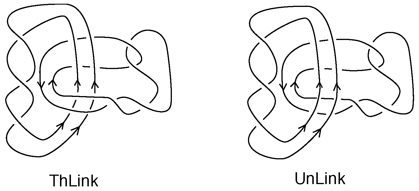
We then show that each generalized invariant can be reformulated in terms of a closed formula, involving summation over evaluations of sublinks of the given link (Theorems 5–7). It is remarkable that the generalized invariants have two such distinct faces, as skein invariants and as closed combinatorial formuli. In this paper, we present both of these points of view and how they are related to state summations and possible relationships with statistical mechanics and applications. These constructions alter the philosophy of classical skein-theoretic techniques, whereby mixed as well as self-crossings in a link diagram would get indiscriminately switched. Using a known skein invariant, one first unlinks all components using the skein relation and then one evaluates on unions of unlinked knots using that skein invariant and at the same time introducing a new variable. This approach could find applications in physical systems where different constituents need to be separated first.

This paper is based on [1] where the reader can find more detailed treatment of much of the theory.

There are not many known skein link invariants in the literature. Skein invariants include: the Alexander–Conway polynomial [2,3], the Jones polynomial [4], and the Homflypt polynomial [5,6,7,8], which specializes to both the Alexander–Conway and the Jones polynomial; there is also the bracket polynomial [9], the Brandt–Lickorish–Millett–Ho polynomial [10], the Dubrovnik polynomial and the Kauffman polynomial [11], which specializes to both the bracket and the Brandt–Lickorish–Millett–Ho polynomial. Finally, we have the Juyumaya–Lambropoulou family of invariants ${\Delta }_{d,D}$, $d\in \mathbb{N}$, for any non-empty subset D of $\mathbb{Z}/d\mathbb{Z}$ [12], and the analogous Chlouveraki–Juyumaya–Karvounis–Lambropoulou invariants ${\mathrm{\Theta }}_d$ and their 3-variable generalization $\mathrm{\Theta }$ [13]. In fact, this last invariant $\mathrm{\Theta }$ was our motivation for constructing the generalized invariants. The invariant $H\left[H\right]$ is in fact the regular isotopy version of the invariant $\mathrm{\Theta }$ and Theorem 1 can be used to provide a self-contained skein theoretic proof of its existence.

The invariant $\mathrm{\Theta }$ was discovered via the following path: In [12] a family of framed link invariants was constructed via a Markov trace on the Yokonuma–Hecke algebras [14], which restrict to the family of classical link invariants $\left\{{\Delta }_{d,D}\right\}$ [15]. These were studied in [15,16], especially their relation to the Homflypt polynomial, P, but topological comparison had not been possible due to algebraic and diagrammatic difficulties. In [13,17,18] another presentation [19] was used for the Yokonuma–Hecke algebra and the related classical link invariants were now denoted ${\mathrm{\Theta }}_d$. The invariants ${\mathrm{\Theta }}_d$ were then recovered via the skein relation of P that can only apply to mixed crossings of a link [13] and they were shown to be distinct from P on links, for $d\ne 1$, but topologically equivalent to P on knots [13,17] (hence also distinct from the Kauffman polynomial). Finally, the family of invariants $\left\{{\mathrm{\Theta }}_d\right\}$, which includes P for $d=1$, was generalized to the new 3-variable skein link invariant $\mathrm{\Theta }$ [13], which is also related to the theory of tied links [20]. A succinct exposition of the above results can be found in [21]. These constructions opened the way to new research directions. Cf. [12,13,15,16,17,19,20,22,23,24,25,26,27,28,29,30,31,32,33,34,35,36,37,38].

Further, in [13] Appendix B, W.B.R. Lickorish provides a closed combinatorial formula for the definition of the invariant $\mathrm{\Theta }$, showing that it is a mixture of Homflypt polynomials and linking numbers of sublinks of a given link. The combinatorial formuli (7), (15) and (16) for the generalized invariants are inspired by the Lickorish formula. These closed formuli are remarkable summations of evaluations on sublinks with certain coefficients, that surprisingly satisfy the analogous mixed skein relations, so they can be regarded by themselves as definitions of the invariants $H\left[H\right]$, $D\left[D\right]$ and $K\left[K\right]$ respectively. Formula (7) shows that the strength of $H\left[H\right]$ against H comes from its ability to distinguish certain sublinks of Homflypt-equivalent links. In [13] a list of six 3-component links are given, which are Homflypt equivalent but are distinguished by the invariant $\mathrm{\Theta }$ and thus also by $H\left[H\right]$.

We proceed with constructing state sum models associated to the generalized skein invariants. A state sum model is a sum over evaluations of combinatorial configurations (the states) related to the given link diagram, such that this sum is equal to the invariant that we wish to compute. The state sums are based on the skein template algorithm, as explained in [39,40], which formalizes the skein theoretic process as an analogue of a statistical mechanics partition function and produces the states to be evaluated. Our state sums use the skein calculation process for the invariants, but have a new property in the present context. They have a double level due to the combination in our invariants of a skein calculation combined with the evaluation of a specific invariant on the knots that are at the bottom of the skein process. If we choose a state sum evaluation of a different kind for this specific invariant, then we obtain a double-level state sum of our new invariant.

The paper concludes with a discussion about possible relationships with reconnection in vortices in fluids, strand switching and replication of DNA, particularly the possible relations with the replication of Kinetoplast DNA, and we discuss the possibility of multiple levels in the quantum Hall effect where one considers the braiding of quasi-particles that are themselves physical subsystems composed of multiple electron vortices centered about magnetic field lines.

The paper is organized as follows: In Section 2 we present the skein theoretic setting of the new skein 3-variable invariants that generalize the regular isotopy version of the Homflypt, the Dubrovnik and the Kauffman polynomials. In Section 3 we give the ambient isotopy reformulations of the generalized link invariants. In Section 4 we adapt the combinatorial formula of Lickorish to our regular isotopy setting for the generalized skein invariants. In Section 5 we define associated state sum models for the new invariants, while in Section 6 the idea about double state summations is articulated. Finally, in Section 7 we discuss the context of statistical mechanics models and partition functions in relation to multiple level state summations and in Section 8 we speculate about possible applications for these ideas.

2. The Skein-Theoretic Setting for the Generalized Invariants

In this section, we define the general regular isotopy invariant for links, $H\left[H\right]$, $D\left[D\right]$ and $K\left[K\right]$, which generalize the regular isotopy version of the Homflypt polynomial, H, the Dubrovnik polynomial, D, and the Kauffman polynomial, K, respectively.

As usual, an oriented link is a link with an orientation specified for each component. In addition, a link diagram is a projection of a link on the plane with only finitely many double points, the crossings, which are endowed with information ‘under/over’. Two link diagrams are regularly isotopic if they differ by planar isotopy and by Reidemeister moves II and III (with all variations of orientations in the case of oriented diagrams). A mixed crossing is a crossing between different components.

2.1. Defining $H\left[H\right]$

Let $\mathcal{L}$ denote the set of classical oriented link diagrams. Let $L_{+}\in \mathcal{L}$ be an oriented diagram with a positive crossing specified and let $L_{-}$ be the same diagram but with that crossing switched. Let also $L_0$ indicate the same diagram but with the smoothing which is compatible with the orientations of the emanating arcs in place of the crossing. See (1). The diagrams $L_{+},L_{-},L_0$ comprise a so-called oriented Conway triple.

(1)

we then have the following:

Theorem 1

(cf. [1]). Let $H(z,a)$ denote the regular isotopy version of the Homflypt polynomial. Then there exists a unique regular isotopy invariant of classical oriented links $H\left[H\right]:\mathcal{L}\to \mathbb{Z}[z,a^{\pm 1},E^{\pm 1}]$, where $z,a$ and E are indeterminates, defined by the following rules:

• On crossings involving different components the following mixed skein relation holds:

  $$H\left[H\right]\left(L_{+}\right)-H\left[H\right]\left(L_{-}\right)=zH\left[H\right]\left(L_0\right),$$

  where $L_{+}$, $L_{-}$, $L_0$ is an oriented Conway triple,
• For a union of r unlinked knots, ${\mathcal{K}}^r:={\bigsqcup }_{i=1}^r{K}_i$, with $r\ge 1$, it holds that:

  $$H\left[H\right]\left({\mathcal{K}}^r\right)=E^{1-r}H\left({\mathcal{K}}^r\right).$$

We recall that the invariant $H(z,a)$ is determined by the following rules:

(H1)

For $L_{+}$, $L_{-}$, $L_0$ an oriented Conway triple, the following skein relation holds:

$$H\left(L_{+}\right)-H\left(L_{-}\right)=zH\left(L_0\right),$$

(H2)

The indeterminate a is the positive curl value for H:

(H3)

On the standard unknot:

$$R(◯)=1.$$

We also recall that the above defining rules imply the following:

(H4)

For a diagram of the unknot, U, H is evaluated by taking:

$$H\left(U\right)=a^{wr\left(U\right)},$$

where $wr\left(U\right)$ denotes the writhe of U—instead of 1 that is the case in the ambient isotopy category.

(H5)

H being the Homflypt polynomial, it is multiplicative on a union of unlinked knots, ${\mathcal{K}}^r:={\bigsqcup }_{i=1}^r{K}_i$. Namely, for $\eta :=\frac{a-a^{-1}}{z}$ we have:

$$H\left({\mathcal{K}}^r\right)={\eta }^{r-1}{\Pi }_{i=1}^{r}H\left(K_i\right).$$

Consequently, the evaluation of $H\left[H\right]$ on the standard unknot is $H\left[H\right](◯)=H(◯)=1$.

Assuming Theorem 1 one can compute $H\left[H\right]$ on any given oriented link diagram $L\in \mathcal{L}$ by applying the following procedure: the skein rule (1) of Theorem 1 can be used to give an evaluation of $H\left[H\right]\left(L_{+}\right)$ in terms of $H\left[H\right]\left(L_{-}\right)$ and $H\left[H\right]\left(L_0\right)$ or of $H\left[H\right]\left(L_{-}\right)$ in terms of $H\left[H\right]\left(L_{+}\right)$ and $H\left[H\right]\left(L_0\right)$. We switch mixed crossings so that the switched diagram is more unlinked than before. Applying this principle recursively we obtain a sum with polynomial coefficients and evaluations of $H\left[H\right]$ on unions of unlinked knots. These are formed by the mergings of components caused by the smoothings in the skein relation (1). To evaluate $H\left[H\right]$ on a given union of unlinked knots we then use the invariant H according to rule (2) of Theorem 1. Note that the appearance of the indeterminate E in rule (2) is the critical difference between $H\left[H\right]$ and H. Finally, evaluations on individual knotted components are done with the use of H via formula (H5) above.

One could specialize the z, the a and the E in Theorem 1 in any way one wishes. For example, if $a=1$ then H specializes to the Alexander–Conway polynomial [2,3]. If $z=\sqrt{a}-1/\sqrt{a}$ then H becomes the unnormalized Jones polynomial [4]. In each case $H\left[H\right]$ can be regarded as a generalization of that polynomial.

The invariant $H\left[H\right]$ generalizes H to a new 3-variable invariant for links. Indeed, $H\left[H\right]$ coincides with the regular isotopy version of the new 3-variable link invariant $\mathrm{\Theta }$ of [13]. On the other hand, by normalizing $H\left[H\right]$ to obtain its ambient isotopy counterpart, we have by Theorem 1 an independent, skein-theoretic proof of the well-definedness of $\mathrm{\Theta }$.

2.2. Defining $D\left[D\right]$ and $K\left[K\right]$

We now consider the class ${\mathcal{L}}^u$ of unoriented link diagrams. For any crossing of a diagram of a link in ${\mathcal{L}}^u$, if we rotate the overcrossing arc counterclockwise it sweeps two regions out of the four. If we join these two regions, this is the A-smoothing of the crossing, while joining the other two regions gives rise to the B-smoothing. Using these conventions, the A-smoothing of $L_{+}$ in (2) below is $L_0$ and the B-smoothing of $L_{+}$ is $L_{\infty }$. Similarly, the A-smoothing of $L_{-}$ is $L_{\infty }$ and the B-smoothing of $L_{-}$ is $L_0$. We shall say that a crossing is of positive type if it produces a horizontal A-smoothing and that it is of negative type if it produces a vertical A-smoothing. Let now $L_{+}$ be an unoriented diagram with a positive type crossing specified and let $L_{-}$ be the same diagram but with that crossing switched. Let also $L_0$ and $L_{\infty }$ indicate the same diagram but with the A-smoothing and the B-smoothing in place of the crossing. See (2). The diagrams $L_{+},L_{-},L_0,L_{\infty }$ comprise a so-called unoriented Conway quadruple.

(2)

In analogy to Theorem 1 we also have the 3-variable generalizations of the regular isotopy versions of the Dubrovnik and the Kauffman polynomials [11]:

Theorem 2

(cf. [1]). Let $D(z,a)$ denote the regular isotopy version of the Dubrovnik polynomial. Then there exists a unique regular isotopy invariant of classical unoriented links $D\left[D\right]:{\mathcal{L}}^u\to \mathbb{Z}[z,a^{\pm 1},E^{\pm 1}]$, where $z,a$ and E are indeterminates, defined by the following rules:

• On crossings involving different components the following skein relation holds:

  $$D\left[D\right]\left(L_{+}\right)-D\left[D\right]\left(L_{-}\right)=z\left(D\left[D\right]\left(L_0\right)-D\left[D\right]\left(L_{\infty }\right)\right),$$

  where $L_{+}$, $L_{-}$, $L_0$, $L_{\infty }$ is an unoriented Conway quadruple,
• For a union of r unlinked knots in ${\mathcal{L}}^u$, ${\mathcal{K}}^r:={\bigsqcup }_{i=1}^r{K}_i$, with $r\ge 1$, it holds that:

  $$D\left[D\right]\left({\mathcal{K}}^r\right)=E^{1-r}D\left({\mathcal{K}}^r\right).$$

We recall that the invariant $D(z,a)$ is determined by the following rules:

(D1)

For $L_{+}$, $L_{-}$, $L_0$, $L_{\infty }$ an unoriented Conway quadruple, the following skein relation holds:

$$D\left(L_{+}\right)-D\left(L_{-}\right)=z\left(D\left(L_0\right)-D\left(L_{\infty }\right)\right),$$

(D2)

The indeterminate a is the positive type curl value for D:

(D3)

On the standard unknot:

$$D(◯)=1.$$

We also recall that the above defining rules imply the following:

(D4)

For a diagram of the unknot, U, D is evaluated by taking

$$D\left(U\right)=a^{wr\left(U\right)},$$

(D5)

D, being the Dubrovnik polynomial, it is multiplicative on a union of unlinked knots, ${\mathcal{K}}^r:={\bigsqcup }_{i=1}^r{K}_i$. Namely, for $\delta :=\frac{a-a^{-1}}{z}+1$ we have:

$$D\left({\mathcal{K}}^r\right)={\delta }^{r-1}{\Pi }_{i=1}^{r}D\left(K_i\right).$$

Consequently, on the standard unknot we evaluate $D\left[D\right](◯)=D(◯)=1$.

The Dubrovnik polynomial, D, is related to the Kauffman polynomial, K, via the following translation formula, observed by W.B.R Lickorish [11]:

$$D\left(L\right)(a,z)={(-1)}^{c\left(L\right)+1}{i}^{-wr\left(L\right)}K\left(L\right)(ia,-iz).$$

(3)

Here, $c\left(L\right)$ denotes the number of components of the link $L\in {\mathcal{L}}^u$, $i^2=-1$, and $wr\left(L\right)$ is the writhe of L for some choice of orientation of L, which is defined as the algebraic sum of all crossings of L. The translation formula is independent of the particular choice of orientation for L. Our theory generalizes also the regular isotopy version of the Kauffman polynomial [11] through the following:

Theorem 3

(cf. [1]). Let $K(z,a)$ denote the regular isotopy version of the Kauffman polynomial. Then there exists a unique regular isotopy invariant of classical unoriented links $K\left[K\right]:{\mathcal{L}}^u\to \mathbb{Z}[z,a^{\pm 1},E^{\pm 1}]$, where $z,a$ and E are indeterminates, defined by the following rules:

• On crossings involving different components the following skein relation holds:

  $$K\left[K\right]\left(L_{+}\right)+K\left[K\right]\left(L_{-}\right)=z\left(K\left[K\right]\left(L_0\right)+K\left[K\right]\left(L_{\infty }\right)\right),$$

  where $L_{+}$, $L_{-}$, $L_0$, $L_{\infty }$ is an unoriented Conway quadruple,
• For a union of r unlinked knots in ${\mathcal{L}}^u$, ${\mathcal{K}}^r:={\bigsqcup }_{i=1}^r{K}_i$, with $r\ge 1$, it holds that:

  $$K\left[K\right]\left({\mathcal{K}}^r\right)=E^{1-r}K\left({\mathcal{K}}^r\right).$$

We recall that the invariant $K(z,a)$ is determined by the following rules:

(K1)

For $L_{+}$, $L_{-}$, $L_0$, $L_{\infty }$ an unoriented Conway quadruple, the following skein relation holds:

$$K\left(L_{+}\right)+K\left(L_{-}\right)=z\left(K\left(L_0\right)+K\left(L_{\infty }\right)\right),$$

(K2)

The indeterminate a is the positive type curl value for K:

(K3)

On the standard unknot:

$$K(◯)=1.$$

We also recall that the above defining rules imply the following:

(K4)

For a diagram of the unknot, U, K is evaluated by taking

$$K\left(U\right)=a^{wr\left(U\right)},$$

(K5)

K, being the Kauffman polynomial, it is multiplicative on a union of unlinked knots, ${\mathcal{K}}^r:={\bigsqcup }_{i=1}^r{K}_i$. Namely, for $\gamma :=\frac{a+a^{-1}}{z}-1$ we have:

$$K\left({\mathcal{K}}^r\right)={\gamma }^{r-1}{\Pi }_{i=1}^{r}K\left(K_i\right).$$

Consequently, on the standard unknot we evaluate $K\left[K\right](◯)=K(◯)=1$.

In Theorems 2 and 3 the basic invariants $D(z,a)$ and $K(z,a)$ could be replaced by specializations of the Dubrovnik and the Kauffman polynomial respectively and, then, the invariants $D\left[D\right]$ and $K\left[K\right]$ can be regarded as generalizations of these specialized polynomials. For example, if $a=1$ then $K(z,1)$ is the Brandt–Lickorish–Millett–Ho polynomial [10] and if $z=A+A^{-1}$ and $a=-A^3$ then K becomes the Kauffman bracket polynomial [9]. In both cases the invariant $K\left[K\right]$ generalizes these polynomials. Furthermore, a formula analogous to (3) relates the generalized invariants $D\left[D\right]$ and $K\left[K\right]$, see (17).

In order to prove Theorems 1–3 one needs to show that the computation of the corresponding generalized invariant can be done solely from the rules of the theorem and that it is independent from any choices involved during the unlinking of different components as well as from the regular isotopy moves. To do this, we specify a computing algorithm to be used; but first we set some terminology.

2.3. Terminology and Notations

A link diagram is called generic if it is ordered, that is, an order $c_1,\dots ,c_r$ is given to its components, directed, that is, a direction is specified on each component, and based, that is, a basepoint is specified on each component, distinct from the double points of the crossings.

A diagram that is the union of r unlinked knots, ${\mathcal{K}}^r:={\bigsqcup }_{i=1}^r{K}_i$, with $r\ge 1$, is said to be a descending stack if, when walking along the components of ${\mathcal{K}}^r$ in their given order, starting from their basepoints and following the specified directions, every mixed crossing is first traversed along its over-arc. Clearly, the structure of a descending stack no longer depends on the choice of basepoints; it is entirely determined by the order of its components. Note also that a descending stack is regularly isotopic to the corresponding split link comprising the r knotted components, $K_i$, where the order of components is no longer relevant. The descending stack of knots associated to a given link diagram L is denoted as $dL$.

2.4. Computing Algorithm for the Generalized Invariants

The generalized invariants are computed on two levels: on the first level one abstracts the corresponding skein relation and applies it only on mixed crossings of a given link diagram. On the second level one evaluates the generalized invariant on unions of unlinked knots, by applying a new rule that uses the corresponding ground invariant and introduces a new variable. More precisely, assuming Theorems 1–3 a generalized invariant can be easily computed on any link diagram L by applying the algorithm below. This algorithm is necessary for proving well-definedness of the invariants.

• (Diagrammatic level) Make L generic by choosing an order for its components and a basepoint and a direction on each component. Start from the basepoint of the first component and go along it in the chosen direction. When arriving at a mixed crossing for the first time along an under-arc we switch it by the mixed skein relation, so that we pass by the mixed crossing along the over-arc. At the same time we smooth the mixed crossing, obtaining a new diagram in which the two components of the crossing merge into one. We repeat for all mixed crossings of the first component. Among all resulting diagrams there is only one with the same number of crossings and the same number of components as the initial diagram and in this one the first component gets unlinked from the rest and lies above all of them. The other resulting diagrams have one less crossing and have the first component fused together with some other component. We proceed similarly with the second component switching all its mixed crossings except for crossings involving the first component. In the end the second component gets unliked from all the rest and lies below the first one and above all others in the maximal crossing diagram, while we also obtain diagrams containing mergings of the second component with others (except component one). We continue in the same manner with all components in order and we also apply this procedure to all product diagrams coming from smoothings of mixed crossings. In the end we obtain the unlinked version of L plus a number of links ℓ with unlinked components resulting from the mergings of different components.
• (Computational level) On the level of the generalized invariant, Rule (1) of Theorems 1–3 tells us how the switching of mixed crossings is controlled. After all applications of the mixed skein relation we obtain a linear sum of the values of the generalized invariant on all the resulting links ℓ with unlinked components. The evaluation of the generalized invariant on each ℓ reduces to the evaluation of the corresponding basic invariant by Rule (2) of Theorems 1–3.

2.5. Sketching the Proof of Theorems 1–3

For proving Theorems 1–3 one must prove that the resulting evaluation for a link diagram L does not depend on the choices made for bringing L to generic form, namely the sequence of mixed crossing changes, the ordering of components and the choice of basepoints, and also that it is invariant under regular isotopy moves. A good guide for this is the skein-theoretic proof of Lickorish–Millett of the well-definedness of the Homflypt polynomial [6], with the necessary adaptations and modifications, taking for granted the well-definedness of the basic invariant. The difference here lies in modifying the original skein method. The original method bottoms out on unlinks, since self-crossings are not distinguished from mixed crossings. In the new method the evaluations bottom out on calculations of the basic invariant on unions of unlinked knots. This difference causes the need of particularly elaborate arguments in proving invariance of the resulting evaluation under the sequence of mixed crossing switches and the order of components in comparison with [6].

Namely, we assume that the statement is valid for all link diagrams of up to $n-1$ crossings, independently of choices made during the evaluation process and of Reidemeister III moves and Reidemeister II moves that do not increase the number of crossings above $n-1$. Our aim is to prove that the statement is valid for all generic link diagrams of up to n crossings, independently of choices, Reidemeister III moves and Reidemeister II moves not increasing above n crossings. We do this by double induction on the total number of crossings of a generic link diagram (which applied to all intermediate diagrams related to smoothings) and on the number of mixed crossing switches needed for bringing the diagram to the form of a descending stack of knots (for which we make the assumption that rule (2) of the corresponding theorem applies).

The interested reader may consult [1] for a detailed exposition.

3. Translations to Ambient Isotopy

In this section, we provide the formuli for the corresponding ambient isotopy invariants, counterparts of the regular isotopy generalized invariants $H\left[H\right]$, $D\left[D\right]$ and $K\left[K\right]$.

3.1. Normalization of $H\left[H\right]$

Let P denote the classical Homflypt polynomial. Then, as we know, one can obtain the ambient isotopy invariant P from its regular isotopy counterpart H via the formula:

$$P\left(L\right):=a^{-wr\left(L\right)}H\left(L\right),$$

where $wr\left(L\right)$ is the total writhe of the oriented diagram L. From our generalized regular isotopy invariant $H\left[H\right]$ one can derive an ambient isotopy invariant $P\left[P\right]$ via:

$$P\left[P\right]\left(L\right):=a^{-wr\left(L\right)}H\left[H\right]\left(L\right).$$

(4)

Then for the invariant $P\left[P\right]$ we have the following:

Theorem 4

(cf. [1]). Let $P(z,a)$ denote the Homflypt polynomial. Then there exists a unique ambient isotopy invariant of classical oriented links $P\left[P\right]:\mathcal{L}\to \mathbb{Z}[z,a^{\pm 1},E^{\pm 1}]$ defined by the following rules:

• On crossings involving different components the following skein relation holds:

  $$aP\left[P\right]\left(L_{+}\right)-a^{-1}P\left[P\right]\left(L_{-}\right)=zP\left[P\right]\left(L_0\right),$$

  where $L_{+}$, $L_{-}$, $L_0$ is an oriented Conway triple.
• For ${\mathcal{K}}^r:={\bigsqcup }_{i=1}^r{K}_i$, a union of r unlinked knots, with $r\ge 1$, it holds that:

  $$P\left[P\right]\left({\mathcal{K}}^r\right)=E^{1-r}P\left({\mathcal{K}}^r\right).$$

Remark 1.

As pointed out in the Introduction, in Theorem 1 we could specialize the z, the a and the E in any way we wish. For example, if $a=1$ then $H(z,1)$ becomes the Alexander–Conway polynomial, while if $z=\sqrt{a}-1/\sqrt{a}$ then $H(\sqrt{a}-1/\sqrt{a},a)$ becomes the unnormalized Jones polynomial. In each case $H\left[H\right]$ can be regarded as a generalization of that polynomial. Furthermore, the ambient isotopy invariant $P\left[P\right]$ coincides with the new 3-variable link invariant $\mathrm{\Theta }(q,\lambda ,E)$ [13], while for $E=1/d$, $P\left[P\right]$ coincides with the invariant ${\mathrm{\Theta }}_d$ [12] (for $E=1$ it coincides with P). So, our invariant $P\left[P\right]$ is stronger than P and it coincides with the invariant Θ. Hence, our proof of the existence of $H\left[H\right]$ provides a direct skein-theoretic proof of the existence of the invariant Θ, without the need of algebraic tools or the theory of tied links. Finally, for $z=\sqrt{a}-1/\sqrt{a}$ the invariant $P\left[P\right]$ can be renamed to $V\left[V\right]$, V denoting the ambient isotopy version of the Jones polynomial, and it coincides with the new 2-variable link invariant $\theta (a,E)$ [33], which generalizes V and is stronger than V. We note that in [13,33] variables q and λ are used instead of z and a, coming from the algebraic background of the invariants, and in that context $a=q^{-2}$ for the invariant θ.

3.2. Normalization of $D\left[D\right]$ and $K\left[K\right]$

Let Y denote the classical ambient isotopy Dubrovnik polynomial. Then, one can obtain the ambient isotopy invariant Y from its regular isotopy counterpart D via the formula:

$$Y\left(L\right):=a^{-wr\left(L\right)}D\left(L\right),$$

where $wr\left(L\right)$ is the total writhe of the diagram L for some choice of orientation of L. Analogously, and letting Z denote Y but with different variable, from our generalized regular isotopy invariant $D\left[D\right]$ one can derive an ambient isotopy invariant $Y\left[Y\right]$ via:

$$Y\left[Y\right]\left(L\right):=a^{-wr\left(L\right)}D\left[D\right]\left(L\right).$$

(5)

In order to have a skein relation one leaves it in regular isotopy form.

As for the Dubrovnik polynomial, one can also define for the Kauffman polynomial the ambient isotopy generalized invariant, counterpart of the regular isotopy generalized invariant $K\left[K\right]$ constructed above. Let K denote the classical regular isotopy Kauffman polynomial. Then, one can obtain the ambient isotopy invariant F from its regular isotopy counterpart K via the formula:

$$F\left(L\right):=a^{-wr\left(L\right)}K\left(L\right),$$

where $wr\left(L\right)$ is the total writhe of the diagram L for some choice of orientation of L. Analogously, and letting S denote F but with different variable, from our generalized regular isotopy invariant $K\left[K\right]$ one can derive an ambient isotopy invariant $F\left[F\right]$ via:

$$F\left[F\right]\left(L\right):=a^{-wr\left(L\right)}K\left[K\right]\left(L\right).$$

(6)

In order to have a skein relation one leaves it in regular isotopy form.

4. Closed Combinatorial Formuli for the Generalized Invariants

4.1. A Closed Formula for $H\left[H\right]$

As we mentioned in the Introduction, in [13] Appendix B, W.B.R. Lickorish provides a closed combinatorial formula for the definition of the invariant $\mathrm{\Theta }=P\left[P\right]$, that uses the Homflypt polynomials and linking numbers of sublinks of a given link. We will give here an analogous formula for our regular isotopy extension $H\left[H\right]$. Namely:

Theorem 5

(cf. [1]). Let L be an oriented link with n components. Then

$$H\left[H\right]\left(L\right)={\displaystyle \sum _{k=1}^n}{\eta }^{k-1}{E}_k\sum _{\pi }H\left(\pi L\right)$$

(7)

where the second summation is over all partitions π of the components of L into k (unordered) subsets and $H\left(\pi L\right)$ denotes the product of the Homflypt polynomials of the k sublinks of L defined by π. Furthermore, $E_k=(E^{-1}-1)(E^{-1}-2)\cdots (E^{-1}-k+1)$ and $\eta =\frac{a-a^{-1}}{z}$.

Proof. 

We present the proof in full detail, as we believe it is instructive and it proves the existence of the generalized invariants. Before proving the result, note the following equalities:

$$\begin{array}{cc}\hfill H(L_1\bigsqcup L_2)& =\eta H\left(L_1\right)H\left(L_2\right),\hfill \\ \hfill H\left[H\right](L_1\bigsqcup L_2)& =\frac{\eta }{E}H\left[H\right]\left(L_1\right)H\left[H\right]\left(L_2\right).\hfill \end{array}$$

In the case where both $L_1$ and $L_2$ are knots the above formuli follow directly from rules (H5) and (2) above. If at least one of $L_1$ and $L_2$ is a true link, then the formuli follow by doing independent skein processes on $L_1$ and $L_2$ for bringing them down to unlinked components, and then using the defining rules above.

Suppose now that a diagram of L is given. The proof is by induction on n and on the number, u, of crossing changes between distinct components required to change L to n unlinked knots. If $n=1$ there is nothing to prove. So assume the result true for $n-1$ components and $u-1$ crossing changes and prove it true for n and u.

The induction starts when $u=0$. Then L is the union of n unlinked components $L_1,\dots ,L_n$. A classic elementary result concerning the Homflypt polynomial shows that $H\left(L\right)={\eta }^{n-1}H\left(L_1\right)\cdots H\left(L_n\right)$. Furthermore, in this situation, for any k and $\pi$, $H\left(\pi L\right)={\eta }^{n-k}H\left(L_1\right)\cdots H\left(L_n\right)$. Note that $H\left[H\right]\left(L\right)=E^{1-n}H\left(L\right)={\eta }^{n-1}{E}^{1-n}H\left(L_1\right)\cdots H\left(L_n\right)$. So it is required to prove that

$${\eta }^{n-1}{E}^{1-n}={\eta }^{n-1}{\displaystyle \sum _{k=1}^n}S(n,k)(E^{-1}-1)(E^{-1}-2)\cdots (E^{-1}-k+1),$$

(8)

where $S(n,k)$ is the number of partitions of a set of n elements into k subsets. Now it remains to prove that:

$$E^{1-n}={\displaystyle \sum _{k=1}^n}S(n,k)(E^{-1}-1)(E^{-1}-2)\cdots (E^{-1}-k+1).$$

(9)

However, in the theory of combinatorics, $S(n,k)$ is known as a Stirling number of the second kind and this required formula is a well known result about such numbers.

Now let $u>0$. Suppose that in a sequence of u crossing changes that changes L, as above, into unlinked knots, the first change is to a crossing c of sign $ϵ$ between components $L_1$ and $L_2$. Let $L^{\prime }$ be L with the crossing changed and $L^0$ be L with the crossing annulled. Now, from the definition of $H\left[H\right]$,

$$H\left[H\right]\left(L\right)=H\left[H\right]\left(L^{\prime }\right)+ϵzH\left[H\right]\left(L^0\right).$$

The induction hypotheses imply that the result is already proved for $L^{\prime }$ and $L^0$ so

$$H\left[H\right]\left(L\right)={\displaystyle \sum _{k=1}^n}{\eta }^{k-1}{E}_k\sum _{{\pi }^{\prime }}H\left({\pi }^{\prime }{L}^{\prime }\right)+ϵz\sum _{k=1}^{n-1}{\eta }^{k-1}{E}_k\sum _{{\pi }^0}H\left({\pi }^0{L}^0\right),$$

(10)

where ${\pi }^{\prime }$ runs through the partitions of the components of $L^{\prime }$ and ${\pi }^0$ through those of $L^0$.

A sublink $X^0$ of $L^0$ can be regarded as a sublink X of L containing $L_1$ and $L_2$ but with $L_1$ and $L_2$ fused together by annulling the crossing at c. Let $X^{\prime }$ be the sublink of $L^{\prime }$ obtained from X by changing the crossing at c. Then

$$H\left(X\right)=H\left(X^{\prime }\right)+ϵzH\left(X^0\right).$$

This means that the second (big) term in (10) is

$${\displaystyle \sum _{k=1}^{n-1}}{\eta }^{k-1}{E}_k\sum _{\rho }\left(H\left(\rho L\right)-H\left({\rho }^{\prime }{L}^{\prime }\right)\right),$$

(11)

where the summation is over all partitions $\rho$ of the components of L for which $L_1$ and $L_2$ are in the same subset and ${\rho }^{\prime }$ is the corresponding partition of the components of $L^{\prime }$.

Note that, for any partition $\pi$ of the components of L inducing partition ${\pi }^{\prime }$ of $L^{\prime }$, if $L_1$ and $L_2$ are in the same subset then we can have a difference between $H\left(\pi L\right)$ and $H\left({\pi }^{\prime }{L}^{\prime }\right)$, but when $L_1$ and $L_2$ are in different subsets then

$$H\left({\pi }^{\prime }{L}^{\prime }\right)=H\left(\pi L\right).$$

(12)

Thus, substituting (11) in (10) we obtain:

$$H\left[H\right]\left(L\right)={\displaystyle \sum _{k=1}^n}{\eta }^{k-1}{E}_k\left(\sum _{{\pi }^{\prime }}H\left({\pi }^{\prime }{L}^{\prime }\right)+\sum _{\rho }\left(H\left(\rho L\right)-H\left({\rho }^{\prime }{L}^{\prime }\right)\right)\right),$$

(13)

where ${\pi }^{\prime }$ runs through all partitions of $L^{\prime }$ and $\rho$ through partitions of L for which $L_1$ and $L_2$ are in the same subset. Note that, for $k=n$ the second sum is zero. Therefore:

$$H\left[H\right]\left(L\right)={\displaystyle \sum _{k=1}^n}{\eta }^{k-1}{E}_k\left(\sum _{{\pi }^{\prime }}H\left({\pi }^{\prime }{L}^{\prime }\right)+\sum _{\rho }H\left(\rho L\right)\right),$$

(14)

where ${\pi }^{\prime }$ runs through only partitions of $L^{\prime }$ for which $L_1$ and $L_2$ are in different subsets and $\rho$ through all partitions of L for which $L_1$ and $L_2$ are in the same subset. Note that in the transition from (13) to (14) the partition set ${\pi }^{\prime }$ changes from all partitions of $L^{\prime }$ to only partitions of $L^{\prime }$ for which $L_1$ and $L_2$ are in different subsets. The equality in (14) follows from the equality in (13) once this difference in partitions is appreciated. Hence, using (14) and also (12), we obtain:

$$H\left[H\right]\left(L\right)={\displaystyle \sum _{k=1}^n}{\eta }^{k-1}{E}_k\sum _{\pi }H\left(\pi L\right)$$

and the induction is complete. ☐

Remark 2.

Note that the combinatorial formula (7) can be regarded by itself as a definition of the invariant $H\left[H\right]$, since the right-hand side of the formula is an invariant of regular isotopy, since H is invariant of regular isotopy. The proof of Theorem 5 then proves that this invariant is $H\left[H\right]$ by verifying the skein relation and axioms for $H\left[H\right]$. In the same way the original Lickorish formula [13] can be regarded as a definition for the invariant $\mathrm{\Theta }=P\left[P\right]$. The two formuli for $H\left[H\right]$ and Θ are interchangeable by writhe normalization, recall (4). Indeed, in translating the regular istotopy Lickorish formula to its ambient isotopy counterpart, we must make writhe compensations for each sublink in a partition and a global writhe compensation for the entire diagram. The products of the global compensation and the local writhe compensations are equal to the linking number coefficients that occur in the ambient isotopy version of the Lickorish formula.

The combinatorial formula (7) is a remarkable summation of evaluations on sublinks with certain coefficients, that surprisingly satisfies the skein relations and order of switchings and evaluations that we have described above.

The reader should note that the formula above (the right hand side) is, by its very definition, a regular isotopy invariant of the link L. This follows from the regular isotopy invariance of H and the well-definedness of summing over all partitions of the link L into k parts. In fact the summations $I_k\left(L\right)={\sum }_{\pi }H\left(\pi L\right)$, where $\pi$ runs over all partitions of L into k parts, are each regular isotopy invariants of L. What is remarkable here is that these all assemble into the new invariant $H\left[H\right]\left(L\right)$ with its striking two-level skein relation. We see from this combinatorial formula that the extra strength of $H\left[H\right]\left(L\right)$ comes from its ability to detect non-triviality of certain sublinks of the link L.

Remark 3.

Since the Lickorish combinatorial formula is itself a link invariant and we prove by induction that it satisfies the two-tiered skein relations of $H\left[H\right]$, this combinatorial formula can be used as a mathematical basis for $H\left[H\right]$. We have chosen to work out the skein theory of $H\left[H\right]$ from first principles, but a reader of this paper may wish to first read the proof of the Lickorish formula and understand the skein relations on that basis. The same remarks apply to the combinatorial formuli for the other two invariants $D\left[D\right]$ and $K\left[K\right]$.

Remark 4.

The combinatorial formula (7) shows that the strength of $H\left[H\right]$ against H comes from its ability to distinguish certain sublinks of Homflypt-equivalent links. In [13] a list of six 3-component links are given, which are Homflypt equivalent but are distinguished by the invariant Θ and thus also by $H\left[H\right]$.

4.2. An Example

Here is an example by the first-named author and D. Goundaroulis showing how $H\left[H\right]$ and the combinatorial formula give extra information in the case of two link components.

Example 1.

We will use the ambient isotopy version of the Jones polynomial $V_K\left(q\right)$ and so first work with a skein calculation of the Jones polynomial, and then with a calculation of the generalized invariant $V\left[V\right]\left(L\right)\left(q\right)$. Recall from Remark 1 that $V\left[V\right]\left(L\right)=\theta (a,E)$ [33]. We use the link $ThLink$ first found by Morwen Thisthlethwaite [41] and generalized by Eliahou, Kauffman and Thistlethwaite [42]. This link of two components is not detectable by the Jones polynomial, but it is detectable by our extension of the Jones polynomial. Note that this link is detectable by the Homflypt polynomial. In doing this calculation we (Louis Kauffman and Dimos Goundaroulis) use Dror Bar Natan’s Knot Theory package for Mathematica. In this package, the Jones polynomial is a function of q and satisfies the skein relation

$$q^{-1}{V}_{K_{+}}\left(q\right)-q{V}_{K_{-}}\left(q\right)=(q^{1/2}-q^{-1/2})V_{K_0}\left(q\right)$$

where $K_{+},K_{-},K_0$ is the usual skein triple. Let

$$a=q^2,z=(q^{1/2}-q^{-1/2}),b=qz,c=q^{-1}z.$$

Then we have the skein expansion formulas:

$$V_{K_{+}}=a{V}_{K_{-}}+b{V}_{K_0}and{V}_{K_{-}}=a^{-1}{V}_{K_{+}}-c{V}_{K_0}.$$

In Figure 1 we show the Thistlethwaite link that is invisible to the Jones polynomial. In the same figure we show an unlink of two components obtained from the Thisthlethwaite link by switching four crossings. In Figure 2 we show the links $K_1,K_2,K_3,K_4$ that are intermediate to the skein process for calculating the invariants of L by first switching only crossings between components. From this it follows that the knots and links in the figures indicated here satisfy the formula

$$V_{ThLink}=b{V}_{K_1}+ab{V}_{K_2}-c{a}^2{V}_{K_3}-ac{V}_{K_4}+V_{Unlinked}.$$

Figure 1. The Thistlethwaite Link and Unlink.

Figure 2. The links $K_1,K_2,K_3,K_4$.

This can be easily verified by the specific values computed in Mathematica:

$$V_{ThLink}=-q^{-1/2}-q^{1/2}$$

$$V_{K_1}=-1+\frac{1}{q^7}-\frac{2}{q^6}+\frac{3}{q^5}-\frac{4}{q^4}+\frac{4}{q^3}-\frac{4}{q^2}+\frac{3}{q}+q$$

$$V_{K_2}=1-\frac{1}{q^9}+\frac{3}{q^8}-\frac{4}{q^7}+\frac{5}{q^6}-\frac{6}{q^5}+\frac{5}{q^4}-\frac{4}{q^3}+\frac{3}{q^2}-\frac{1}{q}$$

$$V_{K_3}=1-\frac{1}{q^9}+\frac{2}{q^8}-\frac{3}{q^7}+\frac{4}{q^6}-\frac{4}{q^5}+\frac{4}{q^4}-\frac{3}{q^3}+\frac{2}{q^2}-\frac{1}{q}$$

$$V_{K_4}=-1-\frac{1}{q^6}+\frac{2}{q^5}-\frac{2}{q^4}+\frac{3}{q^3}-\frac{3}{q^2}+\frac{2}{q}+q$$

$$V_{Unlinked}=\frac{1}{q^{13/2}}-\frac{1}{q^{11/2}}-\frac{1}{q^{7/2}}+\frac{1}{q^{3/2}}-\frac{1}{\sqrt{q}}-q^{3/2}$$

This is computational proof that the Thistlethwaite link is not detectable by the Jones polynomial. If we compute $V\left[V\right]\left(ThLink\right)\left(q\right)$ then we modify the computation to

$$V\left[V\right]\left(ThLink\right)\left(q\right)=b{V}_{K_1}+ab{V}_{K_2}-c{a}^2{V}_{K_3}-ac{V}_{K_4}+E^{-1}{V}_{Unlinked}.$$

and it is quite clear that this is non-trivial when the new variable E is not equal to 1.

On the other hand, the Lickorish formula for this case tells us that, for the regular isotopy version of the Jones polynomial $V^{\prime }\left[V^{\prime }\right]\left(ThLink\right)\left(q\right)$,

$$V^{\prime }\left[V^{\prime }\right]\left(ThLink\right)\left(q\right)=\eta (E^{-1}-1)V_{K_1}^{\prime }{V}_{K_2}^{\prime }\left(q\right)+V_{ThLink}^{\prime }\left(q\right)$$

whenever we evaluate a 2-component link. Note that $\eta (E^{-1}-1)$ is non-zero whenever $E\ne 1$. Thus it is quite clear that the Lickorish formula detects the Thisthlethwaite link since the Jones polynomials of the components of that link are non-trivial. We have, in this example, given two ways to see how the extended invariant detects the link $ThLink$. The first way shows how the detection works in the extended skein theory. The second way shows how it works using the Lickorish formula.

4.3. Closed Formuli for $D\left[D\right]$ and $K\left[K\right]$

As for the case of $H\left[H\right]$, there are analogous formuli for the generalized invariants $D\left[D\right]$ and $K\left[K\right]$.

Theorem 6

(cf. [1]). Let L be an unoriented link with n components. Then

$$D\left[D\right]\left(L\right)={\displaystyle \sum _{k=1}^n}{\delta }^{k-1}{E}_k\sum _{\pi }D\left(\pi L\right)$$

(15)

where the second summation is over all partitions π of the components of L into k (unordered) subsets and $D\left(\pi L\right)$ denotes the product of the Dubrovnik polynomials of the k sublinks of L defined by π. Furthermore, $E_k=(E^{-1}-1)(E^{-1}-2)\cdots (E^{-1}-k+1)$, with $E_1=1$, and $\delta =\frac{a-a^{-1}}{z}+1$.

The proof of Theorem 6 uses similar arguments as the one for Theorem 5. Further, a closed combinatorial formula exists also for the invariant $K\left[K\right]$:

Theorem 7

(cf. [1]). Let L be an unoriented link with n components. Then

$$K\left[K\right]\left(L\right)=i^{wr\left(L\right)}{\displaystyle \sum _{k=1}^n}{\gamma }^{k-1}{E}_k\sum _{\pi }{i}^{-wr\left(\pi L\right)}K\left(\pi L\right).$$

(16)

where the second summation is over all partitions π of the components of L into k (unordered) subsets and $K\left(\pi L\right)$ denotes the product of the Kauffman polynomials of the k sublinks of L defined by π. The term $wr\left(\pi L\right)$ denotes the sum of the writhes of the parts of the partitioned link $\pi L$. Furthermore, $E_k=(E^{-1}-1)(E^{-1}-2)\cdots (E^{-1}-k+1)$, with $E_1=1$, and $\gamma =\frac{a+a^{-1}}{z}-1$.

We prove this Theorem [1] by using the translation formula between the Kauffman and Dubrovnik polynomials and the combinatorial formula that we have already proved for the Dubrovnik polynomial extension $D\left[D\right]$. The following equation is the translation formula from the Dubrovnik to Kauffman polynomial, observed by W.B.R. Lickorish [11]:

$$D\left(L\right)(a,z)={(-1)}^{c\left(L\right)+1}{i}^{-wr\left(L\right)}K\left(L\right)(ia,-iz).$$

Here, $c\left(L\right)$ denotes the number of components of L, $i^2=-1$, and $wr\left(L\right)$ is the writhe of L for some choice of orientation of L. The translation formula is independent of the particular choice of orientation for L. By the same token, we have the following formula translating the Kauffman polynomial to the Dubrovnik polynomial.

$$K\left(L\right)(a,z)={(-1)}^{c\left(L\right)+1}{i}^{wr\left(L\right)}D\left(L\right)(-ia,iz).$$

These formulas are proved by checking them on basic loop values and then using induction via the skein formulas for the two polynomials. This same method of proof shows that the same translation occurs between our generalizations of the Kauffman polynomial $K\left[K\right]$ and the Dubrovnik polynomial $D\left[D\right]$. In particular, we have

$$D\left[D\right]\left(L\right)(a,z)={(-1)}^{c\left(L\right)+1}{i}^{-wr\left(L\right)}K\left[K\right]\left(L\right)(ia,-iz)$$

(17)

and

$$K\left[K\right]\left(L\right)(a,z)={(-1)}^{c\left(L\right)+1}{i}^{wr\left(L\right)}D\left[D\right]\left(L\right)(-ia,iz).$$

Note that the formuli (15) and (16) can be regarded by themselves as definitions of the invariants $D\left[D\right]$ and $K\left[K\right]$ respectively, since the right-hand sides of the formuli are invariants of regular isotopy, since D and K are invariants of regular isotopy. Furthermore, Remark 4 applies also for the invariants $D\left[D\right]$ and $K\left[K\right]$.

Remark 5.

As noted in the Introduction, in Theorems 2 and 3 the basic invariants $D(z,a)$ and $K(z,a)$ could be replaced by specializations of the Dubrovnik and the Kauffman polynomial respectively and, then, the invariants $D\left[D\right]$ and $K\left[K\right]$ can be regarded as generalizations of these specialized polynomials. For example, if $a=1$ then $K(z,1)$ is the Brandt–Lickorish–Millett–Ho polynomial and if $z=A+A^{-1}$ and $a=-A^3$ then $K(A+A^{-1},-A^3)$ is the Kauffman bracket polynomial. In both cases the invariant $K\left[K\right]$ generalizes these polynomials.

5. State Sum Models

In this section, we present state sum models for the generalized regular isotopy invariant $H\left[H\right]$ of Theorem 1. A state sum model is a sum over evaluations of combinatorial configurations (the states) related to the given link diagram, such that this sum is equal to the invariant that we wish to compute. The definitions for the state sum will be given in Section 5.2. The state sum we use depends on the skein template algorithm (see [39,40]) that effectively produces the states to be evaluated. The skein template algorithm is detailed in Section 5.1.

In fact, we will consider the lower level invariant to be H or any specialization of H and we will be denoting it generically by $R(w,a)$. Thus we will write $H\left[R\right]$ to indicate that we have specialized the lower level invariant. This liberty is justified by the 4-variable framework of [1] and it is useful in applications and computations. Everything we do in the remainder of the paper applies to the generalized Dubrovnik and Kauffman polynomials, $D\left[D\right]$ and $K\left[K\right]$, in essentially the same way.

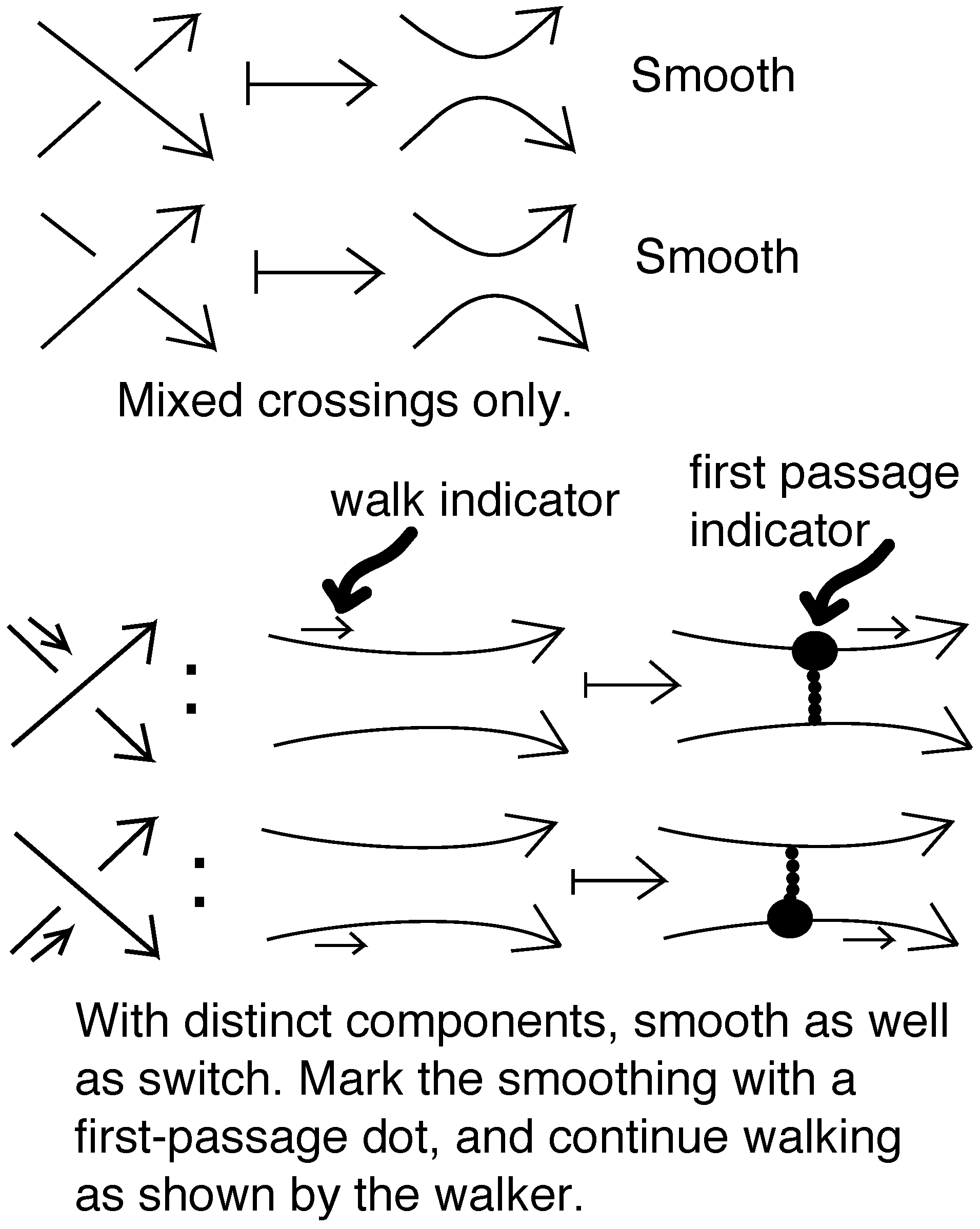
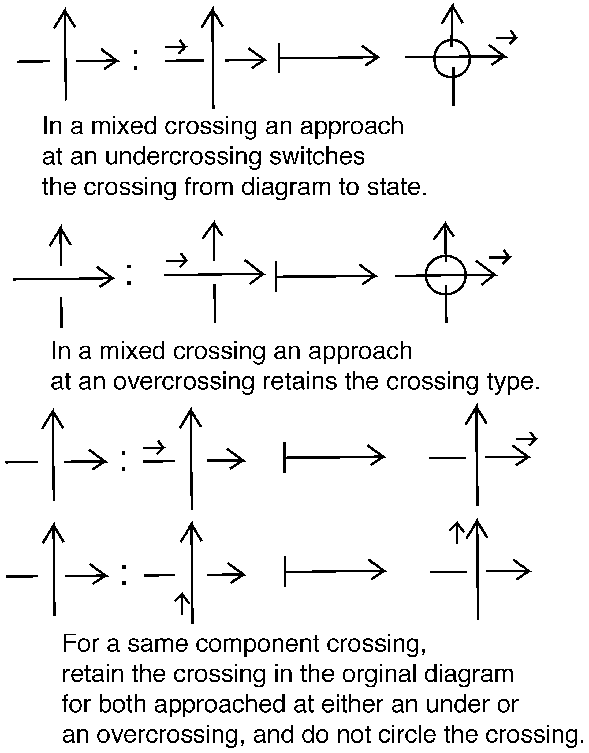
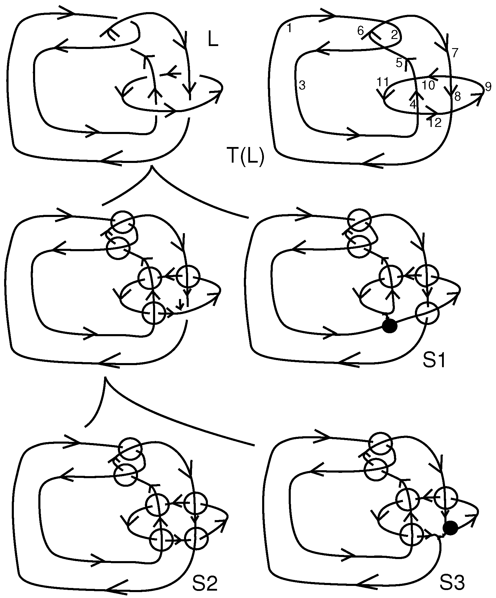
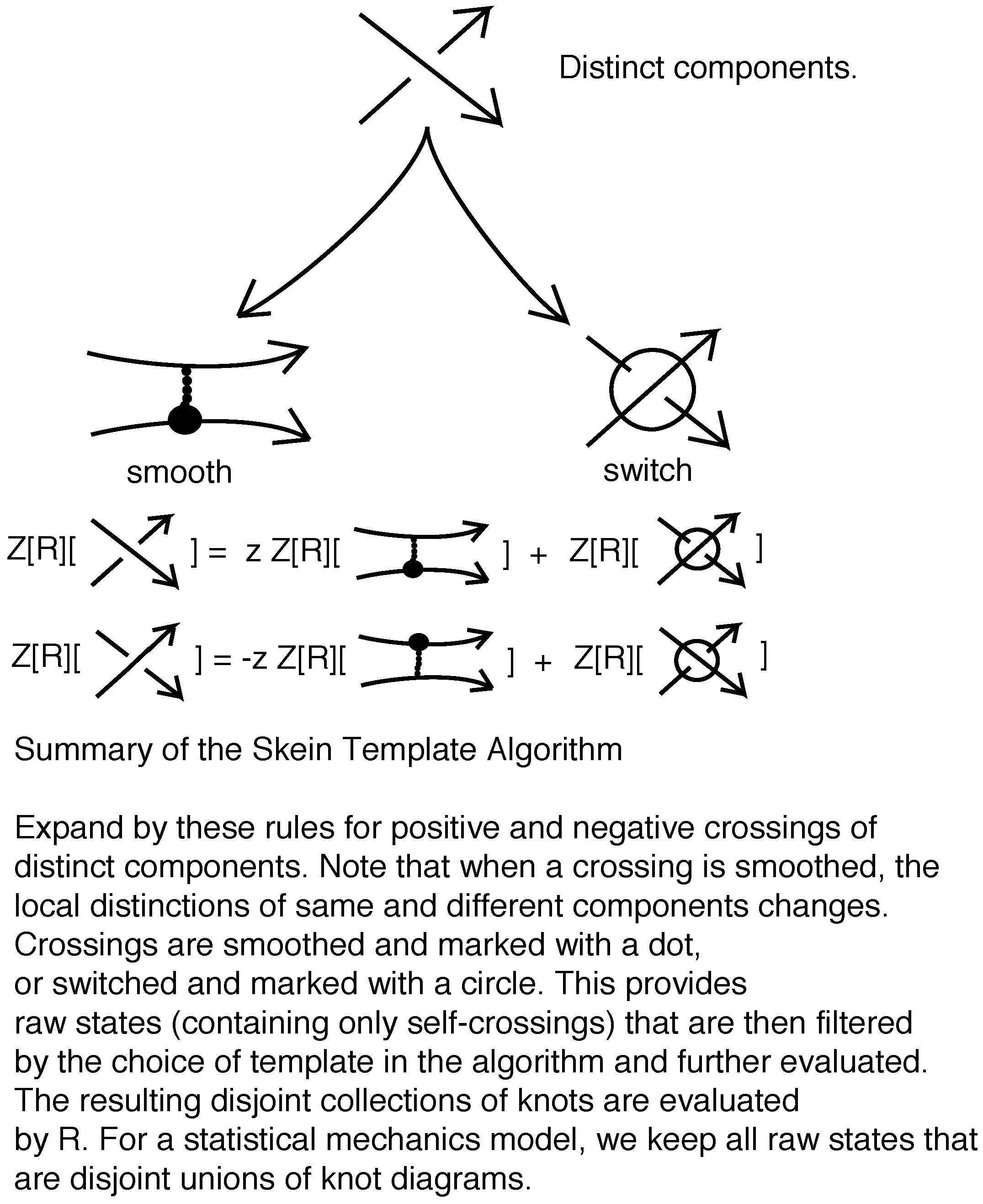
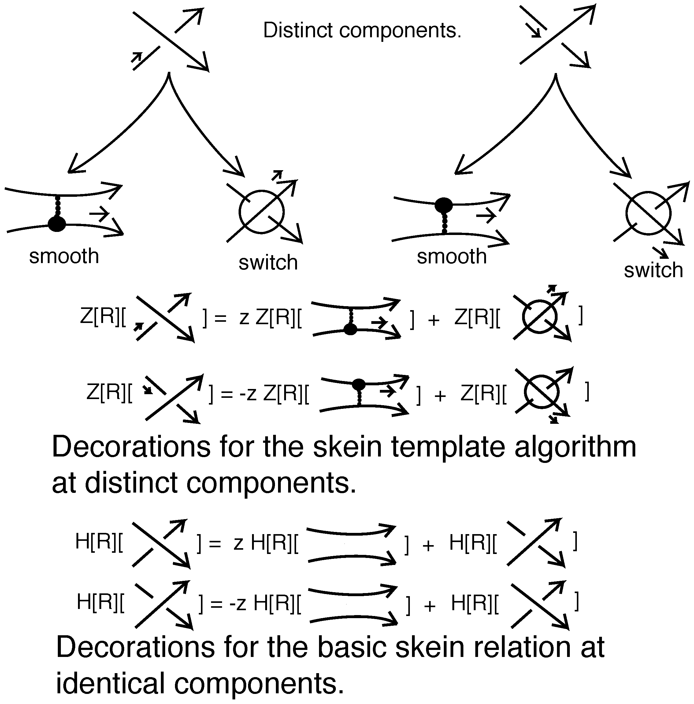
Definition 1.

Let L denote a diagram of an oriented link. The oriented smoothing of a crossing is the replacement of the crossing by the smoothing that is consistent with the orientations of its two arcs. See Figure 3 top. Pre-states, $\widehat{S}$, for L are obtained by successively smoothing or switching mixed crossings (a mixed crossing is a crossing between two components of the link). That is, one begins by choosing a mixed crossing and replacing it by smoothing it and switching it, see Figure 4 top. The smoothing is decorated as in Figure 3, so that there is a dot that discriminates whether the smoothing comes from a positive or a negative crossing. The process of placing the dot is related to walking along the diagram. That walk only allows a smoothing at a mixed crossing that is approached along an undercrossing arc as shown in Figure 3. After the smoothing is produced, that walk and the dotting are related as shown in Figure 3. The reasons for these conventions will be clarified below, where we explain a process that encodes the skein calculation of the invariants. The switched crossing is circled to indicate that it has been chosen by this skein process, see Figure 5. Then one chooses another mixed crossing in each of the resulting diagrams and applies the same procedure. New self-crossings can appear after a smoothing. A completed pre-state is obtained when a decorated diagram is reached where all the undecorated crossings are self-crossings. A state, S, for L is a completed pre-state that is obtained with respect to a template as we describe it below. In a state, we are guaranteed that the resulting link diagram is a topological union of unlinked knot diagrams (a stack). In fact, the skein template process will produce exactly a set of states whose evaluations correspond to the skein evaluation of the invariant $H\left[R\right]$.

Figure 3. First passage decoration at mixed crossings.

Figure 4. Decorated state production by the skein template algorithm.

Figure 5. Decorations on walking past a crossing in a pre-state.

In the skein template algorithm we produce a specific set of pre-states that we can call states, and show how to compute the link invariant $H\left[R\right]$ from these states by adding up evaluations of each state. The key to producing these pre-states is the template. A template, T, for a link diagram L is an indexed, flattened diagram for L (the underlying universe of L, a 4-valent graph obtained from L by ignoring the over and under crossing data in L) so that the indices are on the edges of the graph. See Figure 6 for an illustration of a template T for the Hopf link. We assume that the indices are distinct elements of an ordered set (for example, the natural numbers). We use the template to decide the order of processing for the pre-state. As we know, the invariant $H\left[R\right]$ itself is independent of this ordering. Take the link diagram L and a template T for L. Process the diagram L to produce pre-states $\widehat{S}$ generated by the template T by starting at the smallest index and walking along the diagram, smoothing and marking as described below.

Figure 6. State production for the Hopf link.

5.1. The Skein Template Algorithm

The skein template algorithm is basically very simple. It is a formalization of the skein calculation process, designed to fix all the choices in this process by the choice of the template T. Then the resulting states are exactly the ends of a skein tree for evaluating $H\left[R\right]$. Each state, as a link diagram, is a stack of knots, ready to be evaluated by R. The product of the vertex weights for the state multiplied by R evaluated on the state is equal to the contribution of that state to the polynomial.

We now detail the skein template algorithm. Consider a link diagram L (view Figure 6 and Figure 7). Label each edge of the projected flat diagram of L from an ordered index set I so that each edge receives a distinct label. We have called this labeled graph the template$T\left(L\right)$. We have defined a pre-state$\widehat{S}$ of L by selecting mixed crossings in L and operating on them according to a walk on the template, starting with the smallest index in the labeling of T. We now go through the skein template algorithm, referring at the same time to specific examples.

Figure 7. Skein template algorithm applied to the Whitehead link.

• Begin walking along the link L, starting at the least available index from $T\left(L\right)$. See Figure 6 and Figure 7.
• When meeting a mixed crossing via an under-crossing arc, produce two new diagrams (see Figure 4 top), one by switching the crossing and circling it (Figure 5) and one by smoothing the crossing and labeling it (Figure 3).
• When traveling through a smoothing, label it by a dot and a connector indicating the place of first passage as shown in Figure 3 and exemplified in Figure 6 and Figure 7. At a smoothing, assign to the smoothing a vertex weight of $+z$ or $-z$ (the weights are indicated in Figure 8).
  

  Figure 8. State evaluation relative to the diagram L.
  We clarify these steps with two examples, the Hopf link and the Whitehead link. See Figure 6 and Figure 7. In these figures, for Step 1 we start at the edge with index 1 and meet a mixed crossing at its under-arc, switching it for one diagram and smoothing it for another. We walk past the smoothing, placing a dot and a connector.
• When meeting a mixed over-crossing, circle the crossing (Figure 5 middle) to indicate that it has been processed and continue the walk.
• When meeting a self-crossing, leave it unmarked (Figure 5 bottom) and continue the walk.
• When a closed path has been traversed in the template, choose the next lowest unused template index and start a new walk. Follow the previous instructions for this walk, only labeling smoothings or circling crossings that have not already been so marked.
• When all paths have been traversed, and the pre-state has no remaining un-processed mixed crossing, the pre-state $\widehat{S}$ is now a state S for L. When we have a state S, it is not hard to see that it consists in an unlinked collection of components in the form of stacks of knots as we have previously described in this paper.
• When a pre-state is finished, there will be no undecorated mixed crossings in the state. All uncircled crossings will be self-crossings and there will also be some marked smoothings. All the smoothings will have non-zero vertex weights ( z, $-z$ or 1) and the pre-state becomes a contributing state for the invariant.
• This state is evaluated by taking the product of the vertex weights and the evaluation of the invariant R on the the link underlying the state after all the decorations have been removed. The skein template process produces a link from the state that is a stack of knots. We give the details in the next section.
• The (unnormalized) invariant $H\left[R\right]$ is the sum over all the evaluations of these states obtained by applying the skein-template algorithm. We will denote this sum by $Z\left[R\right]\left(L\right)$ for a given link L and justify in the discussion below that it is indeed equal to the previously defined $H\left[R\right]\left(L\right)$.

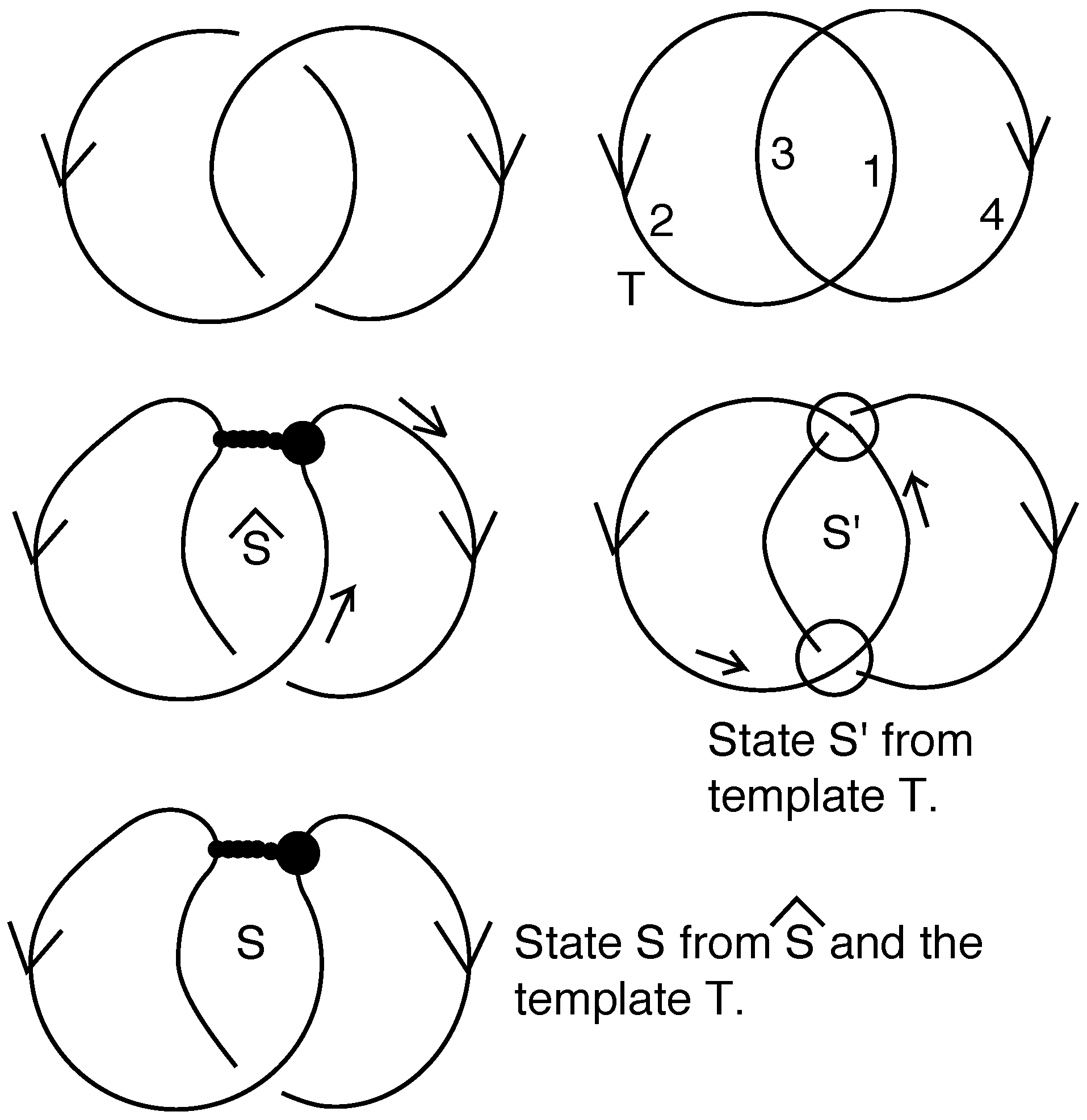
Returning to our example, we have the diagram shown in Figure 6. In this diagram S is a completed state for the initial link L. Note that in forming S we start at 1 in the template and first encounter a mixed under-crossing. This is smoothed to produce the pre-state $\widehat{S}$, and the walk continues to encounter a self-crossing that is left alone. The result is the state S. Moreover, first encounter from 1 meets an under-crossing and we switch and circle this crossing and continue that walk. The next crossing is an over-crossing that is mixed. We circle this crossing and produce the state $S^{\prime }$. The two states S and $S^{\prime }$ are a complete set of states produced by the skein template algorithm for the Hopf link L with this template T.

5.2. The State Summation

We are now in a position to define the state sum.

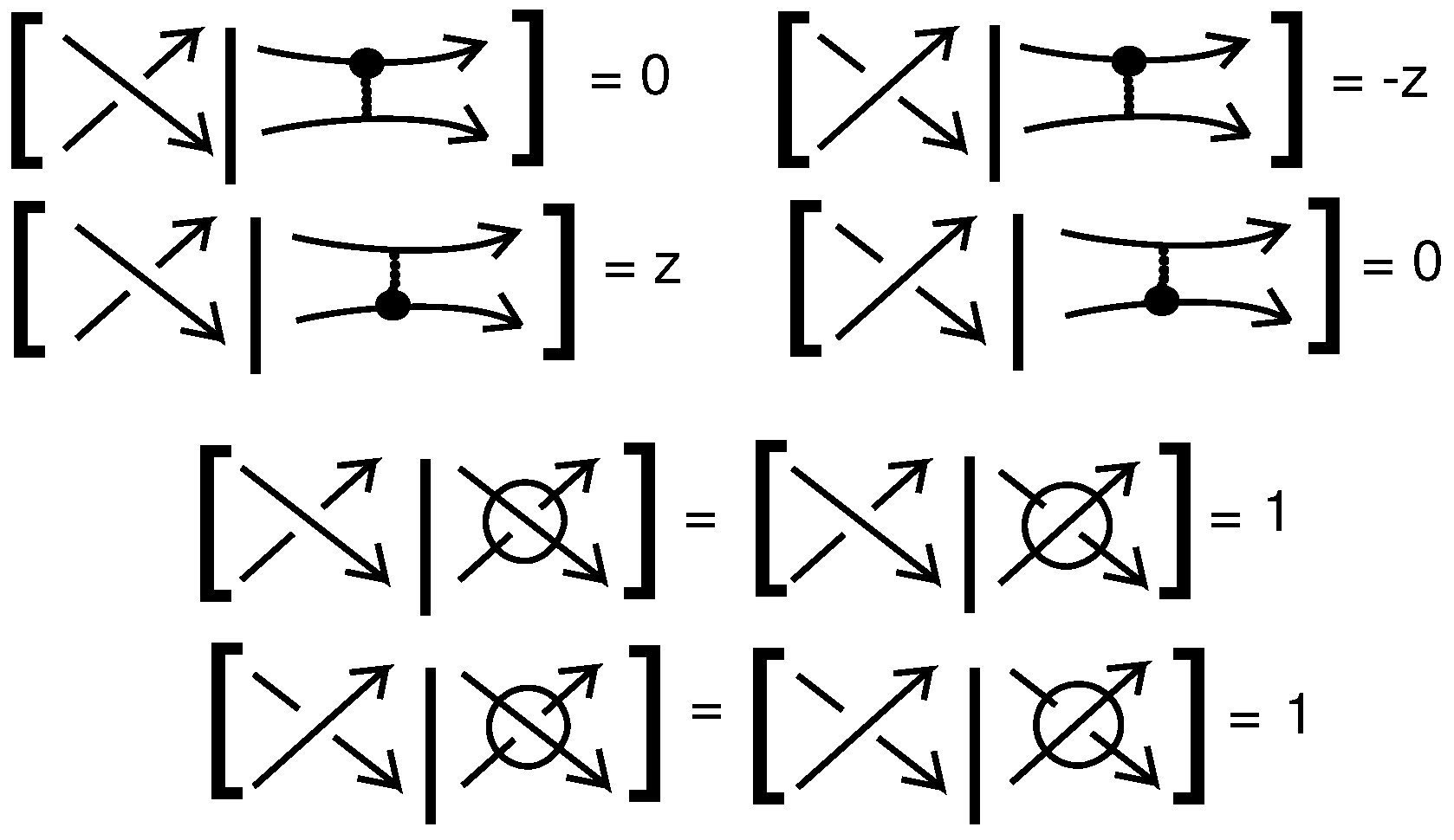
Definition 2.

Let $S\left(L\right)$ denote the collection of states defined by the skein template algorithm for a link diagram L with template T. Given a state S, we shall define an evaluation of S relative to L and the invariant R, denoted by $<L|S>$. The state sum is then defined by

$$Z\left[R\right]\left(L\right)=\sum _{S\in S\left(L\right)}<L|S>.$$

(18)

We will show that $Z\left[R\right]\left(L\right)=H\left[R\right]\left(L\right)$, the regular isotopy invariant that we have defined in earlier sections of the paper. For the specialization R, we let $P\left[R\right]\left(L\right)=a^{-wr\left(L\right)}H\left[R\right]\left(L\right)$ denote the corresponding invariant of ambient isotopy. Thus

$$P\left[R\right]\left(L\right)=a^{-wr\left(L\right)}\sum _{S\in S\left(L\right)}<L|S>$$

(19)

gives the normalized invariant of ambient isotopy in state sum form. The sites of the state S consist in the decorated smoothings and the decorated crossings indicated in Figure 4. Each state evaluation $<L|S>$ consists of two parts. We shall write it in the form

$$<L|S>=[L\left|S\right]\left[R\right|S].$$

(20)

The first part $\left[L\right|S]$ depends only on L and the state S. The second part $\left[R\right|S]$ uses the chosen knot invariant R. We define $\left[L\right|S]$ as a product over the sites of S:

$$\left[L\right|S]=\prod _{\sigma \in sites\left(S\right)}\left[L\right|\sigma ]$$

(21)

where $\left[L\right|\sigma ]$ is defined by the equations in Figure 8, comparing a crossing in L with the corresponding site σ. This means that if a smoothed site has a dot along its lower edge (when oriented from left to right), then its vertex weight is $+z$ and if it has a dot along its upper edge, then it has a vertex weight $-z$. Circled crossings have vertex weights 1. In Figure 8 we have indicated the possibility of vertex weights 0, but these will never occur in the states produced by the skein template algorithm. If we were to sum over a larger set of states, then some of them would be eliminated by this rule. The reader should note that the choice of $+z$ or $-z$ is directly in accord with the rules for the skein relation from a positive crossing or a negative crossing, respectively. We define $\left[R\right|S]$ as a weighted product of the R-evaluations of the components of the state S:

$$\left[R\right|S]=\left[{\displaystyle \prod _{i=1}^k}\rho \left(K_i\right)\right]E^{1-k}$$

(22)

where E is defined previously and

$$\rho \left(K\right)=a^{wr\left(K\right)}R\left(K\right).$$

Here $\{K_1,\dots ,K_k\}$ is the set of component knots of the state S. Recall that each state S is a stacked union of single unlinked component knots $K_i$, $i=1,\dots ,k$, with k depending on the state. In computing $\rho \left(K_i\right)$ we ignore the state decorations and remove the circles from the crossings. With this, we have completed the definition of the state sum.

Note that, by (18) and (20) we assert that

$$Z\left[R\right]\left(L\right)=\sum _{S\in S\left(L\right)}\left[L\right|S]\left[R\right|S].$$

(23)

Remark 6.

If the invariant R is itself generated by a state summation, then we obtain a hybrid state sum for $Z\left[R\right]\left(L\right)$ consisting in the concatenations (in order) of these two structures. We expand on this idea in Section 6.

5.3. Connection of the State Sum with Skein Calculation

We will show that the sum over states corresponds exactly with the results of making a skein calculation that is guided by the template in the skein template algorithm. Thus the template that we have already described works in these two related contexts. In this way we will show that the state summation gives a formula for the invariant $H\left[R\right]\left(L\right)$.

We begin with an illustration for a single abstract crossing as shown in Figure 5. We shall refer to the skein calculation guided by the template as the skein algorithm. In this figure the walker in the skein algorithm (using the template) approaches along the under-crossing line. If the crossing that is met is a self-crossing of the given diagram, then the walker just continues and the crossing is circled. If the crossing that is a mixed crossing of the given diagram, then two new diagrams are produced. In the first case we produce a smoothing with the labelling that indicates a passage along the edge met from the undercrossing arc. In the second case the walker switches the crossing and continues in the same direction as shown in the figure. This creates a bifurcation in the skein tree. Each resulting branch of the skein tree is treated recursively in this way, but first the walker continues on these given branches until it meets an undercrossing of two different components. Using the Homflypt regular isotopy skein relation (recall Theorem 1, rule (1)) we can write an expansion symbolically as shown in Figure 4. Here it is understood that in expanding a crossing,

• its two arcs lie on separate components of the given diagram;
• the walker for the skein process always switches a mixed crossing that the walker approaches as an under-crossing, and never switches a crossing that it approaches as an over-crossing;
• in expanding the crossing, the walker is shifted along according to the illustrations in Figure 4.

Thus, for different components, we have the expansion equation shown in Figure 4. Here, the template takes on the role of letting us make a skein tree of exactly those states that contribute to the state sum for $Z\left[H\right]\left(L\right)$. Indeed, examine Figure 8. The zero-weights correspond to inadmissible states while the z and $-z$ weights correspond to admissible states where the walker approached at an under-crossing; the one-weights correspond to any circled crossing. Thus, we can use the skein algorithm to produce exactly those states that have a non-zero contribution to the state sum.

By using the skein template algorithm and the skein formulas for expansion, we produce a skein tree where the states at the ends of the tree (the original link is the root of the tree) are exactly the states S that give non-zero weights for $\left[L\right|S]$. Thus, by (18) we obtain:

$$Z\left[R\right]\left(L\right)=\sum _{S\in Ends\left(SkeinTree\right)}<L|S>.$$

(24)

Since we have shown that the state sum is identical with the skein algorithm for computing $H\left[R\right]\left(L\right)$, for any link L, this shows that $Z\left[R\right]\left(L\right)=H\left[R\right]\left(L\right)$, as promised. Thus, we have proved:

Theorem 8.

The state sum we have defined as $Z\left[R\right]\left(L\right)$ is identical with the skein evaluation of the invariant $H\left[R\right]\left(L\right)$. We conclude that $Z\left[R\right]\left(L\right)=H\left[R\right]\left(L\right)$, and thus that the skein template algorithm provides a state summation model for the invariant $H\left[R\right]\left(L\right)$.

Proof. 

The state sum $Z\left[R\right]\left(L\right)={\sum }_{S\in S\left(L\right)}<L|S>$ where $S\left(L\right)$ denotes all the states produced by the skein template algorithm, for a choice of template T. $Z\left[R\right]\left(L\right)$ is equal to the sum of evaluations of those states that are produced by the skein algorithm. That is we have the identity

$$Z\left[R\right]\left(L\right)=\sum _{S\in S\left(L\right)}<L|S>=\sum _{S\in Ends\left(SkeinTree\right)}<L|S>=H\left[R\right]\left(L\right).$$

The latter part of this formula follows because the skein template algorithm is a description of a particular skein calculation process for $H\left[R\right]\left(L\right)$, that is faithful to the rules and weights for $H\left[R\right]\left(L\right)$. We have also proved that $H\left[R\right]\left(L\right)$ is invariant and independent of the skein process that produces it. Thus we conclude that $Z\left[R\right]\left(L\right)=H\left[R\right]\left(L\right)$, and thus that the skein template algorithm provides a state summation model for the invariant $H\left[R\right]\left(L\right)$. ☐

Remark 7.

Note that it follows from the proof of Theorem 8 that the calculation of $Z\left[R\right]\left(L\right)=H\left[R\right]\left(L\right)$ is independent of the choice of the template for the skein template algorithm.

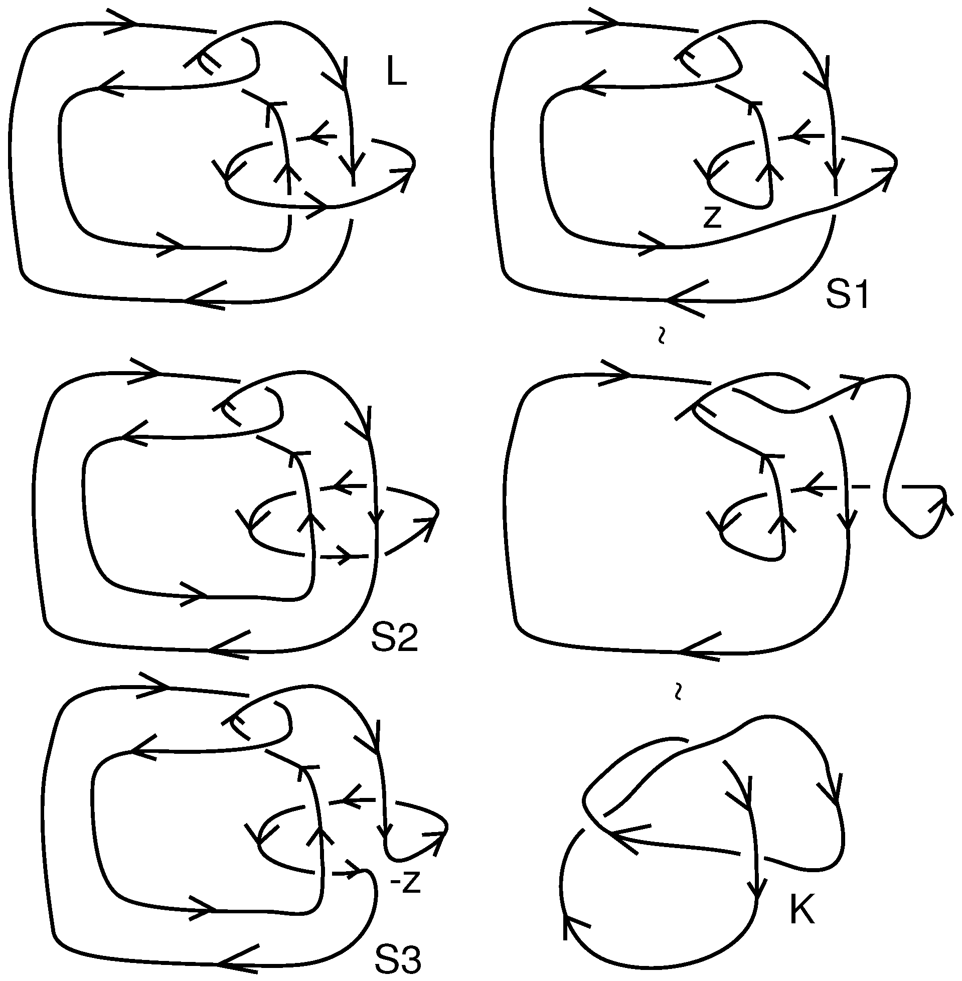
Example 2.

In the example shown in Figure 7 we apply the skein template algorithm to the Whitehead link L. The skein-tree shows that for the given template T there are three contributing states $S_1,S_2,S_3$. $S_1$ is a knot K. $S_2$ is a stacked unlink or two unknotted components. $S_3$ is an unknot. Thus, referring to Figure 9 and using (19) we find the calculation shown below.

$$\begin{gathered} Z\left[R\right]\left(L\right)=z\left[R\right|S_1]+\left[R\right|S_2]-z\left[R\right|S_3] \\ =zR\left(K\right)+a^{-2}(\eta /E)-z{a}^{-3}, \end{gathered}$$

where $\eta =(a-a^{-1})/w$ is defined in rule (5) after Theorem 1 and $K=S_1$.

Figure 9. States for the Whitehead link.

Remark 8.

In the example above we see that any choice of specialization for the invariant R that can distinguish the trivial knot from the trefoil knot K will suffice for our invariant to distinguish the Whitehead link from the trivial link, for which $Z\left[R\right](◯◯)=\eta /E$.

6. Double State Summations

In this section, we consider state summations for our invariant where the invariant R has a state summation expansion. The invariant R has a variable w and a framing variable a. By choosing these variables in particular ways, we can adjust R to be the usual regular isotopy Homflypt polynomial or specializations of the Homflypt polynomial such as a version of the Kauffman bracket polynomial, or the Alexander polynomial, or other invariants. We shall refer to these choices as specializations of R. A given specialization of R may have its own form of state summation. This can be combined with the skein template algorithm that produces states to be evaluated by R. The result is a double state summation.

As in the previous section we have the global state summation (23):

$$Z\left[R\right]\left(L\right)=\sum _{S\in S\left(L\right)}\left[L\right|S]\left[R\right|S]$$

where $\left[R\right|S]$ denotes the evaluation of the invariant R on the union of unlinked knots that is the underlying topological structure of the state S. It is possible that the specialization we are using has itself a state summation that is of interest. In this case we would have a secondary state summation formula of the type

$$\left[R\right|S]=\sum _{\sigma }\left[S\right|\sigma ].$$

(25)

Then, we would have a double state summation for the entire invariant in the schematic form:

$$Z\left[R\right]\left(L\right)=\sum _{S\in S\left(L\right),\sigma \in Rstates\left(S\right)}\left[L\right|S]\left[S\right|\sigma ],$$

(26)

where $Rstates\left(S\right)$ denotes the secondary states for R of the union of unlinked knots that underlies the state S.

Example 3.

Since we use the skein template algorithm to produce the first collection of states $S\in S\left(L\right)$, this double state summation has a precedence ordering with these states produced first, then each S is viewed as a stack of knots and the second state summation is applied. In this section, we will discuss some examples for state summations for R and then give examples of using the double state summation.

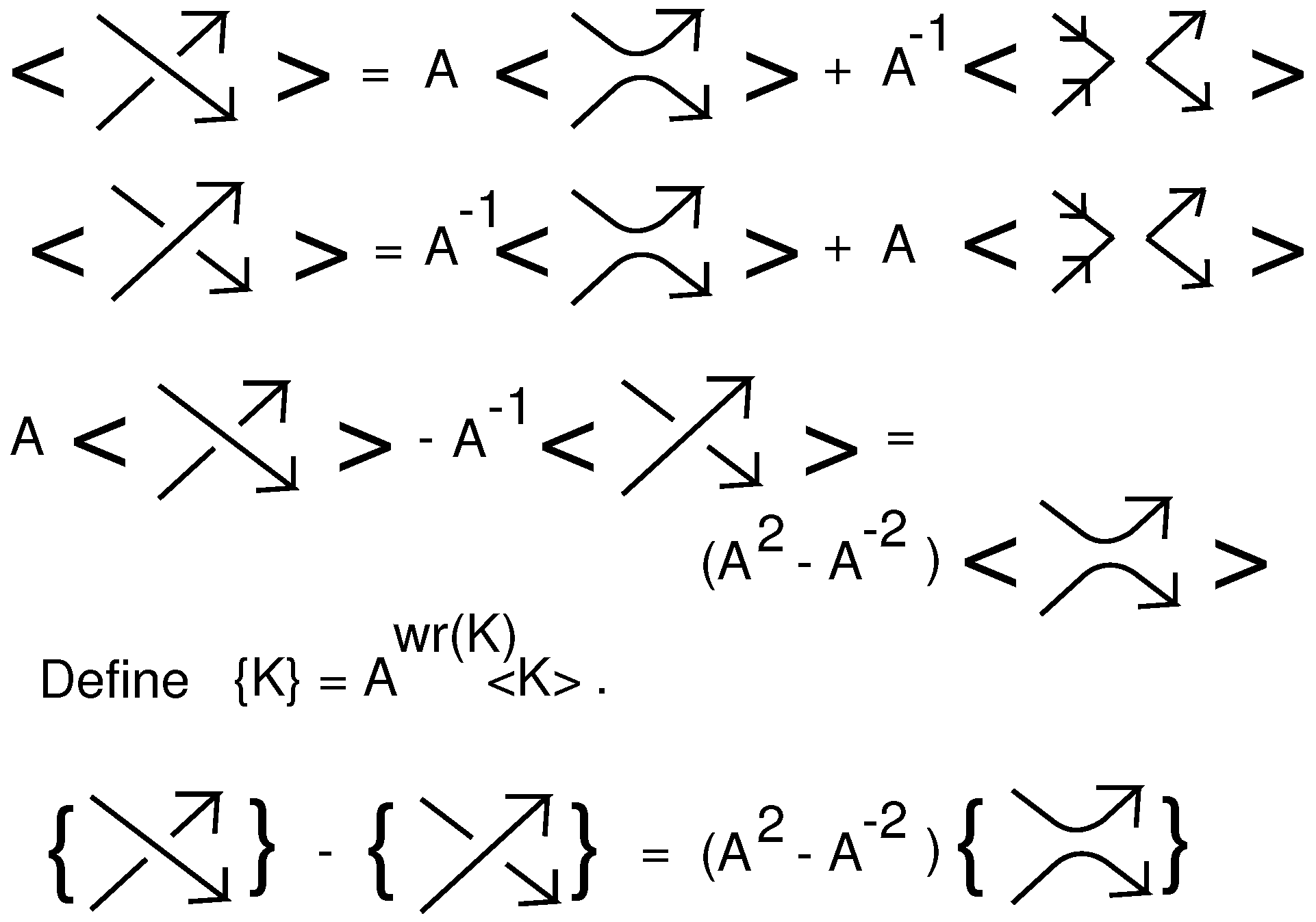
We begin with a state summation for the bracket polynomial that is adapted to our situation. View Figure 10. At the top of the figure we show the standard oriented expansion of the bracket. If the reader is familiar with the usual unoriented expansion [39], then this oriented expansion can be read by forgetting the orientations. The oriented states in this state summation contain smoothings of the type illustrated in the far right hand terms of the two formulas at the top of the figure. We call these disoriented smoothings since two arrowheads point to each other at these sites. Then by multiplying the two equations by A and by $A^{-1}$ respectively, we obtain a difference formula of the type

$$A<K_{+}>-A^{-1}<K_{-}>=(A^2-A^{-2})<K_0>$$

where $K_{+}$ denotes the local appearance of a positive crossing, $K_{-}$ denotes the local appearance of a negative crossing and $K_0$ denotes the local appearance of standard oriented smoothing. The difference equation eliminates the disoriented terms. It then follows easily from this difference equation that if we define a curly bracket by the equation

$$\left\{K\right\}=A^{wr\left(K\right)}<K>$$

where $wr\left(K\right)$ is the diagram writhe (the sum of the signs of the crossings of K), then we have a Homflypt type relation for $\left\{K\right\}$ as follows:

$$\left\{K_{+}\right\}-\left\{K_{-}\right\}=(A^2-A^{-2})\left\{K_0\right\}.$$

(27)

Figure 10. Oriented bracket with Homflypt skein relation.

This means that we can regard $\left\{K\right\}$ as a specialization of the Homflypt polynomial and so we can use it as the invariant R in our double state summation. The state summation for $\left\{K\right\}$ is essentially the same as that for the bracket, as we now detail.

From Figure 10 it is not difficult to see that

$$\left\{K_{+}\right\}=A^2\left\{K_0\right\}+\left\{K_{\infty }\right\}$$

(28)

and

$$\left\{K_{-}\right\}=A^{-2}\left\{K_0\right\}+\left\{K_{\infty }\right\}.$$

(29)

Here $K_{\infty }$ denotes the disoriented smoothing shown in the figure. These formulas then define the state summation for the curly bracket. The reader should note that the difference of these two expansion Equations (28) and (29) is the difference formula (27) for the curly bracket in Homflypt form. The corresponding state summation [40] for these equations is

$$\left\{K\right\}=\sum _{\sigma }{A}^{2s_{+}\left(\sigma \right)-2s_{-}\left(\sigma \right)}{(-A^2-A^{-2})}^{\left|\right|\sigma \left|\right|-1},$$

where σ runs over all choices of oriented and disoriented smoothings of the crossings of the diagram K. Here $s_{+}\left(\sigma \right)$ denotes the number of oriented smoothings of positive crossings and $s_{-}\left(\sigma \right)$ denotes the number of oriented smoothings of negative crossings in the state σ. Further, $\left|\right|\sigma \left|\right|$ denotes the number of loops in the state σ.

With this state sum model in place we can proceed to write a double state sum for the bracket polynomial specialization of our invariant. The formalism of this invariant is after (26), as follows.

$$Z\left[\left\{\right\}\right]\left(L\right)=\sum _{S\in S\left(L\right)}\left[L\right|S]\left\{S\right\}=\sum _{S\in S\left(L\right)}\sum _{\sigma \in smoothings\left(S\right)}\left[L\right|S]A^{2s_{+}\left(\sigma \right)-2s_{-}\left(\sigma \right)}{(-A^2-A^{-2})}^{\left|\right|\sigma \left|\right|-1}.$$

(30)

Here we see the texture of the double state summation. The skein template algorithm produces from the oriented link L the stacks of knots K. Each such stack has a collection of smoothing states, and for each such smoothing state we have the term in the curly bracket expansion formula multiplying a corresponding term from the skein template expansion.

There are many other examples of specific double state summations for other choices of the specialization of the Homflypt polynomial.

Example 4.

For example, we can use the specialized Homflypt state summation based on a solution to the Yang-Baxter equation as explained in [39,40,43].

Example 5.

We could also take the specialization to be the Alexander–Conway polynomial and use the Formal Knot Theory state summation as explained in [44].

All these different cases deserve more exploration, particularly for computing examples of these new invariants.

Remark 9.

The skein template algorithm as well as the double state summation generalizes to the Dubrovnik and Kauffman polynomials, and so applies to our generalizations of them, $D\left[D\right]$ and $K\left[K\right]$, as well. We will take up this computational and combinatorial subject in a sequel to the present paper.

Remark 10.

Consider the combinatorial formula (7). This formula can be regarded itself as a state summation, where the states are the partitions π and the state evaluations are given by the formula and the evaluations of the regular isotopy Homflypt polynomial R on $\pi L$. If we choose a state summation for R or a specialization of R, then this formula becomes a double state summation in the same sense as we discussed above, but without using the skein template algorithm. These double state sums deserve further investigation both for $H\left[R\right]$ and also for the counterparts (15) and (16) for the generalizations $D\left[D\right]$ and $K\left[K\right]$ of the Kauffman and the Dubrovnik polynomials.

7. Statistical Mechanics and Double State Summations

In statistical mechanics, one considers the partition function for a physical system [45]. The partition function $Z_G\left(T\right)$ is a summation over the states $\sigma$ of the system G:

$$Z_G=\sum _{\sigma }{e}^{\frac{-1}{kT}E\left(\sigma \right)}$$

where T is the temperature and k is Bolztmann’s constant. Combinatorial models for simplified systems have been studied intensively since Onsager [46] showed that the partition function for the Ising model for the limits of planar lattices exhibits a phase transition. Onsager’s work showed that very simple physical models, such as the Ising model, can exhibit phase transitions, and this led to the deep research subject of exactly solvable statistical mechanics models [45]. The q-state Potts model [45,47] is an important generalization of the Ising model that is based on q local spins at each site in a graph G. For the Potts model, a state of the graph G is an assignment of spins from $\{1,\dots ,q\}$ to each of the nodes of the graph G. If $\sigma$ is such a state and i denotes the i-th node of the graph G, then we let ${\sigma }_i$ denote the spin assignment to this node. Then the energy of the state $\sigma$ is given by the formula

$$E\left(\sigma \right)=\sum _{⟨i,j⟩}\delta ({\sigma }_i,{\sigma }_j)$$

where $⟨i,j⟩$ denotes an edge in the graph between nodes i and j, and $\delta (x,y)$ is equal to 1 when $x=y$ and equal to 0 otherwise.

Temperley and Lieb [48] proved that the partition function for the Potts model can be calculated using a contraction—deletion algorithm, and so showed that $Z_G$ is a special version of the dichromatic or Tutte polynomial in graph theory. This, in turn, is directly related to the bracket polynomial state sum, and so by generalizing the variables in the bracket state sum and translating the planar graph G into a knot diagram by a medial construction (associating a planar graph to a link diagram via a checkerboard coloring of the diagram so that each shaded region in the checkerboard corresponds to a graphical node and each crossing between shaded regions corresponds to an edge) , one obtains an expression for the Potts model as a bracket summation with new parameters [47]. We wish to discuss the possible statistical mechanical interpretation of our generalized bracket state summation $Z\left[\right\{\left\}\right]$ (see Equation (30)). In order to do this we shall extend the variables of our state sum so that the bracket calculation (for the stacks of knots S that correspond to skein template states) is sufficiently general to support (generalized) Potts models associated with these knots. Accordingly, we add variables to the bracket expansion so that

$$\left\{K_{+}\right\}=x\left\{K_0\right\}+y\left\{K_{\infty }\right\},$$

$$\left\{K_{-}\right\}=x^{\prime }\left\{K_0\right\}+y^{\prime }\left\{K_{\infty }\right\}$$

and the loop value is taken to be D rather than $-A^2-A^{-2}$.

For a given knot in the stack S, the state sum remains well-defined and it now can be specialized to compute a generalized Potts model for a plane graph via a medial graph translation. Letting $R\left(K\right)=\left\{K\right\}$ denote this bracket state sum, we can then form a generalized version of $Z\left[R\right]$ by using the expansion in Figure 11 where we use the raw states of this figure, and we do not filter them by the skein template algorithm, but simply ask that each final state is a union of unlinked knots. The result will then be a combinatorially well-defined double-tier state sum. It is this state sum $Z\left[R\right]$ that can be examined in the light of ideas and techniques in statistical mechanics. The first tier expansion is highly non-local, and just pays attention to dividing up the diagrams so that the first tier of states are each collections of unlinked knots. Then each knot can be regarded as a localized physical system and evaluated with the analogue of a Potts model. This is the logical structure of our double state summation, and it is an open question whether it has a significant physical interpretation.

Figure 11. Raw state production for skein template algorithm.

8. Discussing Applications

We contemplate how these new ideas can be applied to physical situations. We present these indications of possible applications here with the full intent to pursue them in subsequent publications.

• Reconnection (in vortices). In a knotted vortex in a fluid or plasma (for example in solar flares) [49] one has a cascade of changes in the vortex topology as strands of the vortex undergo reconnection. The process goes on until the vortex has degenerated into a disjoint union of unknotted simpler vortices. This cascade or hierarchy of interactions is reminiscent of the way the skein template algorithm proceeds to produce unlinks. Studying reconnection in vortices may be facilitated by making a statistical mechanics summation related to the cascade. Such a summation will be analogous the state summations we have described here.
• In DNA, strand switching using topoisomerase of types I and II is vital for the structure of DNA replication [50]. The mixed interaction of topological change and physical evolution of the molecules in vitro may benefit from a mixed state summation that averages quantities respecting the hierarchy of interactions.
• Remarkably, the process of separation and evaluation that we have described here is analogous to proposed processing of Kinetoplast DNA [51] where there are huge links of DNA circles and these must undergo processes that both unlink them from one another and produce new copies for each circle of DNA. The double-tiered structure of DNA replication for the Kinetoplast chainmail DNA appears to be related to the mathematical patterns of our double state summations. If the reader examines the Wiki on Kinetoplast DNA, he/she will note that Topoisomerase II figures crucially in the self-replication [52].
• We wondered whether we could have physical situations that would have the kind of a mixture that is implicit in this state summation, where the initial skein template state sum yields a sum over R-evaluations, and R may itself have a state summation structure. One possible example in the physical world is a normal statistical mechanical situation, where one can have multiple types of materials, all present together, each having different energetic properties. This can lead to a mixed partition function, possibly not quite ordered in the fashion of our algorithm. This would involve a physical hierarchy of interactions so that there would be a double (or multiple) tier resulting from that hierarchy.
• Mixed state models can occur in physical situations when we work with systems of systems. There are many examples of this multiple-tier situation in systems physical and biological. We look for situations where a double state sum would yield new information. For example, in a quantum Hall system [53], the state of the system is in its quasi-particles, but each quasi-particle is itself a vortex of electrons related to a magnetic field line. So the quasi-particles are themselves localized physical systems. Some of this is summarized in the Laughlin wave function for quantum Hall [53]. This is not a simple situation, but a very significant one. There should be other important examples.

9. Conclusions

We have generalized the known skein polynomials to new and more powerful invariants of links by adopting a new two-level skein procedure. We have shown that these new invariants can also be achieved by special formulas evaluating the original invariants on collections of sublinks of the given initial link. We then show how our new skeining procedure leads to state summation expressions for the invariants and how, if the original invariant is given by a state sum, the new state sums are double level state sums involving a mixture of the two forms of summation. This leads to considerations of statistical mechanics models and also physical and biological processes that have significant multiple levels. We conclude that this way of working with skein invariants has the potential to lead to new insights into physical and biological processes.