A Two-Factor Autoregressive Moving Average Model Based on Fuzzy Fluctuation Logical Relationships

Abstract
1. Introduction
2. Preliminaries
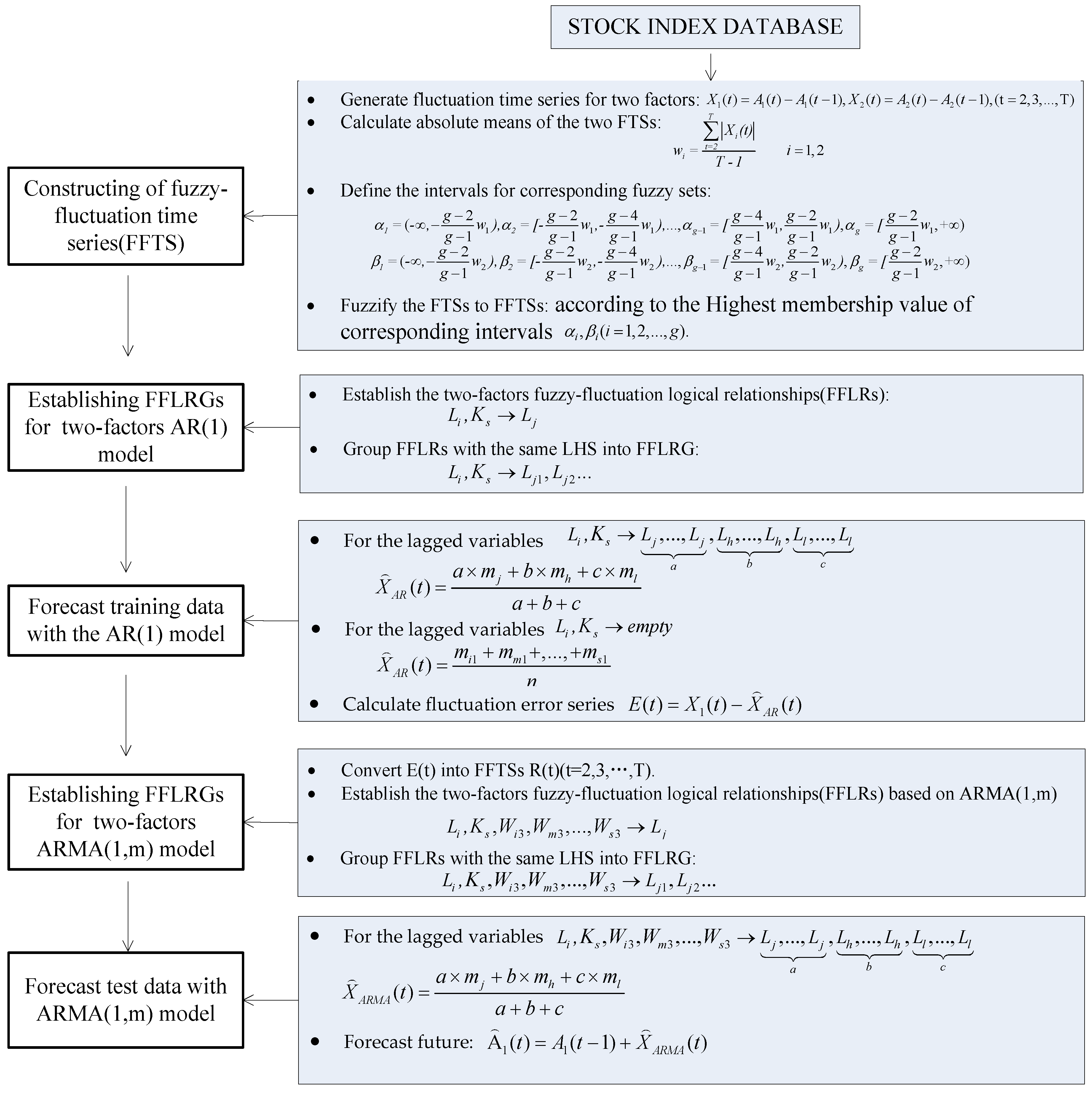
3. New Forecasting Model Based on Two-Factor ARMA(1,m) FFLRs
4. Applications
4.1. Forecasting TAIEX 2004
4.2. Forecasting SHSECI
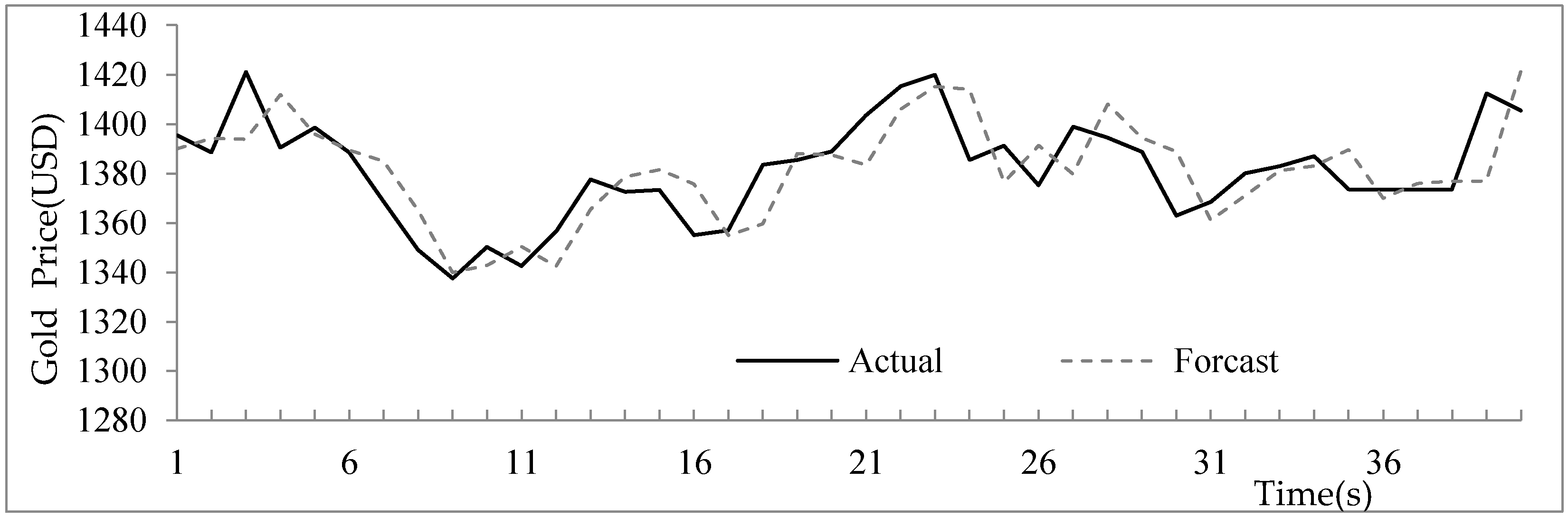
4.3. Forecasting Gold Price
5. Conclusions
Acknowledgments
Author Contributions
Conflicts of Interest
Appendix A

| Date (MM/DD/YYYY) | TAIEX | Fluctuation | Fuzzified | Date (MM/DD/YYYY) | TAIEX | Fluctuation | Fuzzified | Date (MM/DD/YYYY) | TAIEX | Fluctuation | Fuzzified |
|---|---|---|---|---|---|---|---|---|---|---|---|
| 01/02/2004 | 6041.56 | - | - | 04/16/2004 | 6818.20 | 81.41 | 5 | 07/23/2004 | 5373.85 | −14.11 | 3 |
| 01/05/2004 | 6125.42 | 83.86 | 5 | 04/19/2004 | 6779.18 | −39.02 | 2 | 07/26/2004 | 5331.71 | −42.14 | 2 |
| 01/06/2004 | 6144.01 | 18.59 | 4 | 04/20/2004 | 6799.97 | 20.79 | 4 | 07/27/2004 | 5398.61 | 66.90 | 5 |
| 01/07/2004 | 6141.25 | −2.76 | 3 | 04/21/2004 | 6810.25 | 10.28 | 3 | 07/28/2004 | 5383.57 | −15.04 | 3 |
| 01/08/2004 | 6169.17 | 27.92 | 4 | 04/22/2004 | 6732.09 | −78.16 | 1 | 07/29/2004 | 5349.66 | −33.91 | 2 |
| 01/09/2004 | 6226.98 | 57.81 | 5 | 04/23/2004 | 6748.10 | 16.01 | 3 | 07/30/2004 | 5420.57 | 70.91 | 5 |
| 01/12/2004 | 6219.71 | −7.27 | 3 | 04/26/2004 | 6710.70 | −37.40 | 2 | 08/02/2004 | 5350.40 | −70.17 | 1 |
| 01/13/2004 | 6210.22 | −9.49 | 3 | 04/27/2004 | 6646.80 | −63.90 | 1 | 08/03/2004 | 5367.22 | 16.82 | 4 |
| 01/14/2004 | 6274.97 | 64.75 | 5 | 04/28/2004 | 6574.75 | −72.05 | 1 | 08/04/2004 | 5316.87 | −50.35 | 1 |
| 01/15/2004 | 6264.37 | −10.60 | 3 | 04/29/2004 | 6402.21 | −172.54 | 1 | 08/05/2004 | 5427.61 | 110.74 | 5 |
| 01/16/2004 | 6269.71 | 5.34 | 3 | 04/30/2004 | 6117.81 | −284.40 | 1 | 08/06/2004 | 5399.16 | −28.45 | 2 |
| 01/27/2004 | 6384.63 | 114.92 | 5 | 05/03/2004 | 6029.77 | −88.04 | 1 | 08/09/2004 | 5399.45 | 0.29 | 3 |
| 01/28/2004 | 6386.25 | 1.62 | 3 | 05/04/2004 | 6188.15 | 158.38 | 5 | 08/10/2004 | 5393.73 | −5.72 | 3 |
| 01/29/2004 | 6312.65 | −73.60 | 1 | 05/05/2004 | 5854.23 | −333.92 | 1 | 08/11/2004 | 5367.34 | −26.39 | 2 |
| 01/30/2004 | 6375.38 | 62.73 | 5 | 05/06/2004 | 5909.79 | 55.56 | 5 | 08/12/2004 | 5368.02 | 0.68 | 3 |
| 02/02/2004 | 6319.96 | −55.42 | 1 | 05/07/2004 | 6040.26 | 130.47 | 5 | 08/13/2004 | 5389.93 | 21.91 | 4 |
| 02/03/2004 | 6252.23 | −67.73 | 1 | 05/10/2004 | 5825.05 | −215.21 | 1 | 08/16/2004 | 5352.01 | −37.92 | 2 |
| 02/04/2004 | 6241.39 | −10.84 | 3 | 05/11/2004 | 5886.36 | 61.31 | 5 | 08/17/2004 | 5342.49 | −9.52 | 3 |
| 02/05/2004 | 6268.14 | 26.75 | 4 | 05/12/2004 | 5958.79 | 72.43 | 5 | 08/18/2004 | 5427.75 | 85.26 | 5 |
| 02/06/2004 | 6353.35 | 85.21 | 5 | 05/13/2004 | 5918.09 | −40.70 | 2 | 08/19/2004 | 5602.99 | 175.24 | 5 |
| 02/09/2004 | 6463.09 | 109.74 | 5 | 05/14/2004 | 5777.32 | −140.77 | 1 | 08/20/2004 | 5622.86 | 19.87 | 4 |
| 02/10/2004 | 6488.34 | 25.25 | 4 | 05/17/2004 | 5482.96 | −294.36 | 1 | 08/23/2004 | 5660.97 | 38.11 | 4 |
| 02/11/2004 | 6454.39 | −33.95 | 2 | 05/18/2004 | 5557.68 | 74.72 | 5 | 08/26/2004 | 5813.39 | 152.42 | 5 |
| 02/12/2004 | 6436.95 | −17.44 | 2 | 05/19/2004 | 5860.58 | 302.90 | 5 | 08/27/2004 | 5797.71 | −15.68 | 3 |
| 02/13/2004 | 6549.18 | 112.23 | 5 | 05/20/2004 | 5815.33 | −45.25 | 2 | 08/30/2004 | 5788.94 | −8.77 | 3 |
| 02/16/2004 | 6565.37 | 16.19 | 3 | 05/21/2004 | 5964.94 | 149.61 | 5 | 08/31/2004 | 5765.54 | −23.40 | 2 |
| 02/17/2004 | 6600.47 | 35.10 | 4 | 05/24/2004 | 5942.08 | −22.86 | 2 | 09/01/2004 | 5858.14 | 92.60 | 5 |
| 02/18/2004 | 6605.85 | 5.38 | 3 | 05/25/2004 | 5958.38 | 16.30 | 3 | 09/02/2004 | 5852.85 | −5.29 | 3 |
| 02/19/2004 | 6681.52 | 75.67 | 5 | 05/26/2004 | 6027.27 | 68.89 | 5 | 09/03/2004 | 5761.14 | −91.71 | 1 |
| 02/20/2004 | 6665.54 | −15.98 | 3 | 05/27/2004 | 6033.05 | 5.78 | 3 | 09/06/2004 | 5775.99 | 14.85 | 3 |
| 02/23/2004 | 6665.89 | 0.35 | 3 | 05/28/2004 | 6137.26 | 104.21 | 5 | 09/07/2004 | 5846.83 | 70.84 | 5 |
| 02/24/2004 | 6589.23 | −76.66 | 1 | 05/31/2004 | 5977.84 | −159.42 | 1 | 09/08/2004 | 5846.02 | −0.81 | 3 |
| 02/25/2004 | 6644.28 | 55.05 | 5 | 06/01/2004 | 5986.20 | 8.36 | 3 | 09/09/2004 | 5842.93 | −3.09 | 3 |
| 02/26/2004 | 6693.25 | 48.97 | 4 | 06/02/2004 | 5875.67 | −110.53 | 1 | 09/10/2004 | 5846.19 | 3.26 | 3 |
| 02/27/2004 | 6750.54 | 57.29 | 5 | 06/03/2004 | 5671.45 | −204.22 | 1 | 09/13/2004 | 5928.22 | 82.03 | 5 |
| 03/01/2004 | 6888.43 | 137.89 | 5 | 06/04/2004 | 5724.89 | 53.44 | 5 | 09/14/2004 | 5919.77 | −8.45 | 3 |
| 03/02/2004 | 6975.26 | 86.83 | 5 | 06/07/2004 | 5935.82 | 210.93 | 5 | 09/15/2004 | 5871.07 | −48.70 | 2 |
| 03/03/2004 | 6932.17 | −43.09 | 2 | 06/08/2004 | 5986.76 | 50.94 | 5 | 09/16/2004 | 5891.05 | 19.98 | 4 |
| 03/04/2004 | 7034.10 | 101.93 | 5 | 06/09/2004 | 5965.70 | −21.06 | 2 | 09/17/2004 | 5818.39 | −72.66 | 1 |
| 03/05/2004 | 6943.68 | −90.42 | 1 | 06/10/2004 | 5867.51 | −98.19 | 1 | 09/20/2004 | 5864.54 | 46.15 | 4 |
| 03/08/2004 | 6901.48 | −42.20 | 2 | 06/11/2004 | 5735.07 | −132.44 | 1 | 09/21/2004 | 5949.26 | 84.72 | 5 |
| 03/09/2004 | 6973.90 | 72.42 | 5 | 06/14/2004 | 5574.08 | −160.99 | 1 | 09/22/2004 | 5970.18 | 20.92 | 4 |
| 03/10/2004 | 6874.91 | −98.99 | 1 | 06/15/2004 | 5646.49 | 72.41 | 5 | 09/23/2004 | 5937.25 | −32.93 | 2 |
| 03/11/2004 | 6879.11 | 4.20 | 3 | 06/16/2004 | 5560.16 | −86.33 | 1 | 09/24/2004 | 5892.21 | −45.04 | 2 |
| 03/12/2004 | 6800.24 | −78.87 | 1 | 06/17/2004 | 5664.35 | 104.19 | 5 | 09/27/2004 | 5849.22 | −42.99 | 2 |
| 03/15/2004 | 6635.98 | −164.26 | 1 | 06/18/2004 | 5569.29 | −95.06 | 1 | 09/29/2004 | 5809.75 | −39.47 | 2 |
| 03/16/2004 | 6589.72 | −46.26 | 2 | 06/21/2004 | 5556.54 | −12.75 | 3 | 09/30/2004 | 5845.69 | 35.94 | 4 |
| 03/17/2004 | 6577.98 | −11.74 | 3 | 06/23/2004 | 5729.30 | 172.76 | 5 | 10/01/2004 | 5945.35 | 99.66 | 5 |
| 03/18/2004 | 6787.03 | 209.05 | 5 | 06/24/2004 | 5779.09 | 49.79 | 4 | 10/04/2004 | 6077.96 | 132.61 | 5 |
| 03/19/2004 | 6815.09 | 28.06 | 4 | 06/25/2004 | 5802.55 | 23.46 | 4 | 10/05/2004 | 6081.01 | 3.05 | 3 |
| 03/22/2004 | 6359.92 | −455.17 | 1 | 06/28/2004 | 5709.84 | −92.71 | 1 | 10/06/2004 | 6060.61 | −20.40 | 2 |
| 03/23/2004 | 6172.89 | −187.03 | 1 | 06/29/2004 | 5741.52 | 31.68 | 4 | 10/07/2004 | 6103.00 | 42.39 | 4 |
| 03/24/2004 | 6213.56 | 40.67 | 4 | 06/30/2004 | 5839.44 | 97.92 | 5 | 10/08/2004 | 6102.16 | −0.84 | 3 |
| 03/25/2004 | 6156.73 | −56.83 | 1 | 07/01/2004 | 5836.91 | −2.53 | 3 | 10/11/2004 | 6089.28 | −12.88 | 3 |
| 03/26/2004 | 6132.62 | −24.11 | 2 | 07/02/2004 | 5746.70 | −90.21 | 1 | 10/12/2004 | 5979.56 | −109.72 | 1 |
| 03/29/2004 | 6474.11 | 341.49 | 5 | 07/05/2004 | 5659.78 | −86.92 | 1 | 10/13/2004 | 5963.07 | −16.49 | 3 |
| 03/30/2004 | 6494.71 | 20.60 | 4 | 07/06/2004 | 5733.57 | 73.79 | 5 | 10/14/2004 | 5831.07 | −132.00 | 1 |
| 03/31/2004 | 6522.19 | 27.48 | 4 | 07/07/2004 | 5727.78 | −5.79 | 3 | 10/15/2004 | 5820.82 | −10.25 | 3 |
| 04/01/2004 | 6523.49 | 1.30 | 3 | 07/08/2004 | 5713.39 | −14.39 | 3 | 10/18/2004 | 5772.12 | −48.70 | 2 |
| 04/02/2004 | 6545.54 | 22.05 | 4 | 07/09/2004 | 5777.72 | 64.33 | 5 | 10/19/2004 | 5807.79 | 35.67 | 4 |
| 04/05/2004 | 6682.73 | 137.19 | 5 | 07/12/2004 | 5758.74 | −18.98 | 2 | 10/20/2004 | 5788.34 | −19.45 | 2 |
| 04/06/2004 | 6635.54 | −47.19 | 2 | 07/13/2004 | 5685.57 | −73.17 | 1 | 10/21/2004 | 5797.24 | 8.90 | 3 |
| 04/07/2004 | 6646.74 | 11.20 | 3 | 07/14/2004 | 5623.65 | −61.92 | 1 | 10/22/2004 | 5774.67 | −22.57 | 2 |
| 04/08/2004 | 6672.86 | 26.12 | 4 | 07/15/2004 | 5542.80 | −80.85 | 1 | 10/26/2004 | 5662.88 | −111.79 | 1 |
| 04/09/2004 | 6620.36 | −52.50 | 1 | 07/16/2004 | 5502.14 | −40.66 | 2 | 10/27/2004 | 5650.97 | −11.91 | 3 |
| 04/12/2004 | 6777.78 | 157.42 | 5 | 07/19/2004 | 5489.10 | −13.04 | 3 | 10/28/2004 | 5695.56 | 44.59 | 4 |
| 04/13/2004 | 6794.33 | 16.55 | 3 | 07/20/2004 | 5325.68 | −163.42 | 1 | 10/29/2004 | 5705.93 | 10.37 | 3 |
| 04/14/2004 | 6880.18 | 85.85 | 5 | 07/21/2004 | 5409.13 | 83.45 | 5 | ||||
| 04/15/2004 | 6736.79 | −143.39 | 1 | 07/22/2004 | 5387.96 | −21.17 | 2 |
| Date (MM/DD/YYYY) | TAIEX | Fluctuation | Fuzzified | Date (MM/DD/YYYY) | TAIEX | Fluctuation | Fuzzified | Date (MM/DD/YYYY) | TAIEX | Fluctuation | Fuzzified |
|---|---|---|---|---|---|---|---|---|---|---|---|
| 01/02/2004 | 10409.85 | - | - | 04/14/2004 | 10377.95 | −3.33 | 3 | 07/26/2004 | 9961.92 | −0.30 | 3 |
| 01/05/2004 | 10544.07 | 134.22 | 5 | 04/15/2004 | 10397.46 | 19.51 | 4 | 07/27/2004 | 10085.14 | 123.22 | 5 |
| 01/06/2004 | 10538.66 | −5.41 | 3 | 04/16/2004 | 10451.97 | 54.51 | 5 | 07/28/2004 | 10117.07 | 31.93 | 4 |
| 01/07/2004 | 10529.03 | −9.63 | 3 | 04/19/2004 | 10437.85 | −14.12 | 2 | 07/29/2004 | 10129.24 | 12.17 | 3 |
| 01/08/2004 | 10592.44 | 63.41 | 5 | 04/20/2004 | 10314.50 | −123.35 | 1 | 07/30/2004 | 10139.71 | 10.47 | 3 |
| 01/09/2004 | 10458.89 | −133.55 | 1 | 04/21/2004 | 10317.27 | 2.77 | 3 | 08/02/2004 | 10179.16 | 39.45 | 4 |
| 01/12/2004 | 10485.18 | 26.29 | 4 | 04/22/2004 | 10461.20 | 143.93 | 5 | 08/03/2004 | 10120.24 | −58.92 | 1 |
| 01/13/2004 | 10427.18 | −58.00 | 1 | 04/23/2004 | 10472.84 | 11.64 | 3 | 08/04/2004 | 10126.51 | 6.27 | 3 |
| 01/14/2004 | 10538.37 | 111.19 | 5 | 04/26/2004 | 10444.73 | −28.11 | 2 | 08/05/2004 | 9963.03 | −163.48 | 1 |
| 01/15/2004 | 10553.85 | 15.48 | 4 | 04/27/2004 | 10478.16 | 33.43 | 4 | 08/06/2004 | 9815.33 | −147.70 | 1 |
| 01/16/2004 | 10600.51 | 46.66 | 5 | 04/28/2004 | 10342.60 | −135.56 | 1 | 08/09/2004 | 9814.66 | −0.67 | 3 |
| 01/20/2004 | 10528.66 | −71.85 | 1 | 04/29/2004 | 10272.27 | −70.33 | 1 | 08/10/2004 | 9944.67 | 130.01 | 5 |
| 01/21/2004 | 10623.62 | 94.96 | 5 | 04/30/2004 | 10225.57 | −46.70 | 1 | 08/11/2004 | 9938.32 | −6.35 | 3 |
| 01/22/2004 | 10623.18 | −0.44 | 3 | 05/03/2004 | 10314.00 | 88.43 | 5 | 08/12/2004 | 9814.59 | −123.73 | 1 |
| 01/23/2004 | 10568.29 | −54.89 | 1 | 05/04/2004 | 10317.20 | 3.20 | 3 | 08/13/2004 | 9825.35 | 10.76 | 3 |
| 01/26/2004 | 10702.51 | 134.22 | 5 | 05/05/2004 | 10310.95 | −6.25 | 3 | 08/16/2004 | 9954.55 | 129.20 | 5 |
| 01/27/2004 | 10609.92 | −92.59 | 1 | 05/06/2004 | 10241.26 | −69.69 | 1 | 08/17/2004 | 9972.83 | 18.28 | 4 |
| 01/28/2004 | 10468.37 | −141.55 | 1 | 05/07/2004 | 10117.34 | −123.92 | 1 | 08/18/2004 | 10083.15 | 110.32 | 5 |
| 01/29/2004 | 10510.29 | 41.92 | 5 | 05/10/2004 | 9990.02 | −127.32 | 1 | 08/19/2004 | 10040.82 | −42.33 | 1 |
| 01/30/2004 | 10488.07 | −22.22 | 2 | 05/11/2004 | 10019.47 | 29.45 | 4 | 08/20/2004 | 10110.14 | 69.32 | 5 |
| 02/02/2004 | 10499.18 | 11.11 | 3 | 05/12/2004 | 10045.16 | 25.69 | 4 | 08/23/2004 | 10073.05 | −37.09 | 2 |
| 02/03/2004 | 10505.18 | 6.00 | 3 | 05/13/2004 | 10010.74 | −34.42 | 2 | 08/24/2004 | 10098.63 | 25.58 | 4 |
| 02/04/2004 | 10470.74 | −34.44 | 2 | 05/14/2004 | 10012.87 | 2.13 | 3 | 08/25/2004 | 10181.74 | 83.11 | 5 |
| 02/05/2004 | 10495.55 | 24.81 | 4 | 05/17/2004 | 9906.91 | −105.96 | 1 | 08/26/2004 | 10173.41 | −8.33 | 3 |
| 02/06/2004 | 10593.03 | 97.48 | 5 | 05/18/2004 | 9968.51 | 61.60 | 5 | 08/27/2004 | 10195.01 | 21.60 | 4 |
| 02/09/2004 | 10579.03 | −14.00 | 2 | 05/19/2004 | 9937.71 | −30.80 | 2 | 08/30/2004 | 10122.52 | −72.49 | 1 |
| 02/10/2004 | 10613.85 | 34.82 | 4 | 05/20/2004 | 9937.64 | −0.07 | 3 | 08/31/2004 | 10173.92 | 51.40 | 5 |
| 02/11/2004 | 10737.70 | 123.85 | 5 | 05/21/2004 | 9966.74 | 29.10 | 4 | 09/01/2004 | 10168.46 | −5.46 | 3 |
| 02/12/2004 | 10694.07 | −43.63 | 1 | 05/24/2004 | 9958.43 | −8.31 | 3 | 09/02/2004 | 10290.28 | 121.82 | 5 |
| 02/13/2004 | 10627.85 | −66.22 | 1 | 05/25/2004 | 10117.62 | 159.19 | 5 | 09/03/2004 | 10260.20 | −30.08 | 2 |
| 02/17/2004 | 10714.88 | 87.03 | 5 | 05/26/2004 | 10109.89 | −7.73 | 3 | 09/07/2004 | 10341.16 | 80.96 | 5 |
| 02/18/2004 | 10671.99 | −42.89 | 1 | 05/27/2004 | 10205.20 | 95.31 | 5 | 09/08/2004 | 10313.36 | −27.80 | 2 |
| 02/19/2004 | 10664.73 | −7.26 | 3 | 05/28/2004 | 10188.45 | −16.75 | 2 | 09/09/2004 | 10289.10 | −24.26 | 2 |
| 02/20/2004 | 10619.03 | −45.70 | 1 | 06/01/2004 | 10202.65 | 14.20 | 4 | 09/10/2004 | 10313.07 | 23.97 | 4 |
| 02/23/2004 | 10609.62 | −9.41 | 3 | 06/02/2004 | 10262.97 | 60.32 | 5 | 09/13/2004 | 10314.76 | 1.69 | 3 |
| 02/24/2004 | 10566.37 | −43.25 | 1 | 06/03/2004 | 10195.91 | −67.06 | 1 | 09/14/2004 | 10318.16 | 3.40 | 3 |
| 02/25/2004 | 10601.62 | 35.25 | 4 | 06/04/2004 | 10242.82 | 46.91 | 5 | 09/15/2004 | 10231.36 | −86.80 | 1 |
| 02/26/2004 | 10580.14 | −21.48 | 2 | 06/07/2004 | 10391.08 | 148.26 | 5 | 09/16/2004 | 10244.49 | 13.13 | 3 |
| 02/27/2004 | 10583.92 | 3.78 | 3 | 06/08/2004 | 10432.52 | 41.44 | 5 | 09/17/2004 | 10284.46 | 39.97 | 4 |
| 03/01/2004 | 10678.14 | 94.22 | 5 | 06/09/2004 | 10368.44 | −64.08 | 1 | 09/20/2004 | 10204.89 | −79.57 | 1 |
| 03/02/2004 | 10591.48 | −86.66 | 1 | 06/10/2004 | 10410.10 | 41.66 | 5 | 09/21/2004 | 10244.93 | 40.04 | 4 |
| 03/03/2004 | 10593.11 | 1.63 | 3 | 06/14/2004 | 10334.73 | −75.37 | 1 | 09/22/2004 | 10109.18 | −135.75 | 1 |
| 03/04/2004 | 10588.00 | −5.11 | 3 | 06/15/2004 | 10380.43 | 45.70 | 5 | 09/23/2004 | 10038.90 | −70.28 | 1 |
| 03/05/2004 | 10595.55 | 7.55 | 3 | 06/16/2004 | 10379.58 | −0.85 | 3 | 09/24/2004 | 10047.24 | 8.34 | 3 |
| 03/08/2004 | 10529.48 | −66.07 | 1 | 06/17/2004 | 10377.52 | −2.06 | 3 | 09/27/2004 | 9988.54 | −58.70 | 1 |
| 03/09/2004 | 10456.96 | −72.52 | 1 | 06/18/2004 | 10416.41 | 38.89 | 4 | 09/28/2004 | 10077.40 | 88.86 | 5 |
| 03/10/2004 | 10296.89 | −160.07 | 1 | 06/21/2004 | 10371.47 | −44.94 | 1 | 09/29/2004 | 10136.24 | 58.84 | 5 |
| 03/11/2004 | 10128.38 | −168.51 | 1 | 06/22/2004 | 10395.07 | 23.60 | 4 | 09/30/2004 | 10080.27 | −55.97 | 1 |
| 03/12/2004 | 10240.08 | 111.70 | 5 | 06/23/2004 | 10479.57 | 84.50 | 5 | 10/01/2004 | 10192.65 | 112.38 | 5 |
| 03/15/2004 | 10102.89 | −137.19 | 1 | 06/24/2004 | 10443.81 | −35.76 | 2 | 10/04/2004 | 10216.54 | 23.89 | 4 |
| 03/16/2004 | 10184.67 | 81.78 | 5 | 06/25/2004 | 10371.84 | −71.97 | 1 | 10/05/2004 | 10177.68 | −38.86 | 2 |
| 03/17/2004 | 10300.30 | 115.63 | 5 | 06/28/2004 | 10357.09 | −14.75 | 2 | 10/06/2004 | 10239.92 | 62.24 | 5 |
| 03/18/2004 | 10295.78 | −4.52 | 3 | 06/29/2004 | 10413.43 | 56.34 | 5 | 10/07/2004 | 10125.40 | −114.52 | 1 |
| 03/19/2004 | 10186.60 | −109.18 | 1 | 06/30/2004 | 10435.48 | 22.05 | 4 | 10/08/2004 | 10055.20 | −70.20 | 1 |
| 03/22/2004 | 10064.75 | −121.85 | 1 | 07/01/2004 | 10334.16 | −101.32 | 1 | 10/11/2004 | 10081.97 | 26.77 | 4 |
| 03/23/2004 | 10063.64 | −1.11 | 3 | 07/02/2004 | 10282.83 | −51.33 | 1 | 10/12/2004 | 10077.18 | −4.79 | 3 |
| 03/24/2004 | 10048.23 | −15.41 | 2 | 07/06/2004 | 10219.34 | −63.49 | 1 | 10/13/2004 | 10002.33 | −74.85 | 1 |
| 03/25/2004 | 10218.82 | 170.59 | 5 | 07/07/2004 | 10240.29 | 20.95 | 4 | 10/14/2004 | 9894.45 | −107.88 | 1 |
| 03/26/2004 | 10212.97 | −5.85 | 3 | 07/08/2004 | 10171.56 | −68.73 | 1 | 10/15/2004 | 9933.38 | 38.93 | 4 |
| 03/29/2004 | 10329.63 | 116.66 | 5 | 07/09/2004 | 10213.22 | 41.66 | 5 | 10/18/2004 | 9956.32 | 22.94 | 4 |
| 03/30/2004 | 10381.70 | 52.07 | 5 | 07/12/2004 | 10238.22 | 25.00 | 4 | 10/19/2004 | 9897.62 | −58.70 | 1 |
| 03/31/2004 | 10357.70 | −24.00 | 2 | 07/13/2004 | 10247.59 | 9.37 | 3 | 10/20/2004 | 9886.93 | −10.69 | 3 |
| 04/01/2004 | 10373.33 | 15.63 | 4 | 07/14/2004 | 10208.80 | −38.79 | 2 | 10/21/2004 | 9865.76 | −21.17 | 2 |
| 04/02/2004 | 10470.59 | 97.26 | 5 | 07/15/2004 | 10163.16 | −45.64 | 1 | 10/22/2004 | 9757.81 | −107.95 | 1 |
| 04/05/2004 | 10558.37 | 87.78 | 5 | 07/16/2004 | 10139.78 | −23.38 | 2 | 10/25/2004 | 9749.99 | −7.82 | 3 |
| 04/06/2004 | 10570.81 | 12.44 | 3 | 07/19/2004 | 10094.06 | −45.72 | 1 | 10/26/2004 | 9888.48 | 138.49 | 5 |
| 04/07/2004 | 10480.15 | −90.66 | 1 | 07/20/2004 | 10149.07 | 55.01 | 5 | 10/27/2004 | 10002.03 | 113.55 | 5 |
| 04/08/2004 | 10442.03 | −38.12 | 2 | 07/21/2004 | 10046.13 | −102.94 | 1 | 10/28/2004 | 10004.54 | 2.51 | 3 |
| 04/12/2004 | 10515.56 | 73.53 | 5 | 07/22/2004 | 10050.33 | 4.20 | 3 | 10/29/2004 | 10027.47 | 22.93 | 4 |
| 04/13/2004 | 10381.28 | −134.28 | 1 | 07/23/2004 | 9962.22 | −88.11 | 1 |
Appendix B
| Date | TAIEX Group | Dow Jones Group | Actual | Forecast | Fluctuation | Fuzzified | Date | TAIEX Group | Dow Jones Group | Actual | Forecast | Fluctuation | Fuzzified |
|---|---|---|---|---|---|---|---|---|---|---|---|---|---|
| TAIEX | TAIEX | Group of Fluctuation | TAIEX | TAIEX | Group of Fluctuation | ||||||||
| 01/05/2004 | 3 | 3 | 6125.42 | 6041.56 | 83.86 | 5 | 06/03/2004 | 1 | 5 | 5671.45 | 5871.95 | −200.50 | 1 |
| 01/06/2004 | 5 | 5 | 6144.01 | 6144.81 | −0.80 | 3 | 06/04/2004 | 1 | 1 | 5724.89 | 5671.45 | 53.44 | 5 |
| 01/07/2004 | 4 | 3 | 6141.25 | 6118.88 | 22.37 | 4 | 06/07/2004 | 5 | 5 | 5935.82 | 5744.28 | 191.54 | 5 |
| 01/08/2004 | 3 | 3 | 6169.17 | 6141.25 | 27.92 | 4 | 06/08/2004 | 5 | 5 | 5986.76 | 5955.21 | 31.55 | 4 |
| 01/09/2004 | 4 | 5 | 6226.98 | 6213.84 | 13.14 | 3 | 06/09/2004 | 5 | 5 | 5965.70 | 6006.15 | −40.45 | 2 |
| 01/12/2004 | 5 | 1 | 6219.71 | 6214.80 | 4.91 | 3 | 06/10/2004 | 2 | 1 | 5867.51 | 5961.51 | −94.00 | 1 |
| 01/13/2004 | 3 | 4 | 6210.22 | 6216.66 | −6.44 | 3 | 06/11/2004 | 1 | 5 | 5735.07 | 5863.79 | −128.72 | 1 |
| 01/14/2004 | 3 | 1 | 6274.97 | 6210.22 | 64.75 | 5 | 06/14/2004 | 1 | 1 | 5574.08 | 5735.07 | −160.99 | 1 |
| 01/15/2004 | 5 | 5 | 6264.37 | 6294.36 | −29.99 | 2 | 06/15/2004 | 1 | 1 | 5646.49 | 5574.08 | 72.41 | 5 |
| 01/16/2004 | 3 | 4 | 6269.71 | 6261.32 | 8.39 | 3 | 06/16/2004 | 5 | 5 | 5560.16 | 5665.88 | −105.72 | 1 |
| 01/27/2004 | 3 | 5 | 6384.63 | 6298.42 | 86.21 | 5 | 06/17/2004 | 1 | 3 | 5664.35 | 5560.16 | 104.19 | 5 |
| 01/28/2004 | 5 | 1 | 6386.25 | 6372.45 | 13.80 | 3 | 06/18/2004 | 5 | 3 | 5569.29 | 5644.81 | −75.52 | 1 |
| 01/29/2004 | 3 | 1 | 6312.65 | 6386.25 | −73.60 | 1 | 06/21/2004 | 1 | 4 | 5556.54 | 5582.69 | −26.15 | 2 |
| 01/30/2004 | 1 | 5 | 6375.38 | 6308.93 | 66.45 | 5 | 06/23/2004 | 3 | 1 | 5729.30 | 5556.54 | 172.76 | 5 |
| 02/02/2004 | 5 | 2 | 6319.96 | 6341.88 | −21.92 | 2 | 06/24/2004 | 5 | 5 | 5779.09 | 5748.69 | 30.40 | 4 |
| 02/03/2004 | 1 | 3 | 6252.23 | 6319.96 | −67.73 | 1 | 06/25/2004 | 4 | 2 | 5802.55 | 5784.67 | 17.88 | 4 |
| 02/04/2004 | 1 | 3 | 6241.39 | 6252.23 | −10.84 | 3 | 06/28/2004 | 4 | 1 | 5709.84 | 5787.66 | −77.82 | 1 |
| 02/05/2004 | 3 | 2 | 6268.14 | 6234.69 | 33.45 | 4 | 06/29/2004 | 1 | 2 | 5741.52 | 5698.67 | 42.85 | 4 |
| 02/06/2004 | 4 | 4 | 6353.35 | 6284.89 | 68.46 | 5 | 06/30/2004 | 4 | 5 | 5839.44 | 5786.19 | 53.25 | 5 |
| 02/09/2004 | 5 | 5 | 6463.09 | 6372.74 | 90.35 | 5 | 07/01/2004 | 5 | 4 | 5836.91 | 5849.01 | −12.10 | 3 |
| 02/10/2004 | 5 | 2 | 6488.34 | 6429.59 | 58.75 | 5 | 07/02/2004 | 3 | 1 | 5746.70 | 5836.91 | −90.21 | 1 |
| 02/11/2004 | 4 | 4 | 6454.39 | 6505.09 | −50.70 | 1 | 07/05/2004 | 1 | 1 | 5659.78 | 5746.70 | −86.92 | 1 |
| 02/12/2004 | 2 | 5 | 6436.95 | 6471.14 | −34.19 | 2 | 07/06/2004 | 1 | 1 | 5733.57 | 5659.78 | 73.79 | 5 |
| 02/13/2004 | 2 | 1 | 6549.18 | 6432.76 | 116.42 | 5 | 07/07/2004 | 5 | 1 | 5727.78 | 5721.39 | 6.39 | 3 |
| 02/16/2004 | 5 | 1 | 6565.37 | 6537.00 | 28.37 | 4 | 07/08/2004 | 3 | 4 | 5713.39 | 5724.73 | −11.34 | 3 |
| 02/17/2004 | 3 | 3 | 6600.47 | 6565.37 | 35.10 | 4 | 07/09/2004 | 3 | 1 | 5777.72 | 5713.39 | 64.33 | 5 |
| 02/18/2004 | 4 | 5 | 6605.85 | 6645.14 | −39.29 | 2 | 07/12/2004 | 5 | 5 | 5758.74 | 5797.11 | −38.37 | 2 |
| 02/19/2004 | 3 | 1 | 6681.52 | 6605.85 | 75.67 | 5 | 07/13/2004 | 2 | 4 | 5685.57 | 5741.99 | −56.42 | 1 |
| 02/20/2004 | 5 | 3 | 6665.54 | 6661.98 | 3.56 | 3 | 07/14/2004 | 1 | 3 | 5623.65 | 5685.57 | −61.92 | 1 |
| 02/23/2004 | 3 | 1 | 6665.89 | 6665.54 | 0.35 | 3 | 07/15/2004 | 1 | 2 | 5542.80 | 5612.48 | −69.68 | 1 |
| 02/24/2004 | 3 | 3 | 6589.23 | 6665.89 | −76.66 | 1 | 07/16/2004 | 1 | 1 | 5502.14 | 5542.80 | −40.66 | 2 |
| 02/25/2004 | 1 | 1 | 6644.28 | 6589.23 | 55.05 | 5 | 07/19/2004 | 2 | 2 | 5489.10 | 5477.01 | 12.09 | 3 |
| 02/26/2004 | 5 | 4 | 6693.25 | 6653.85 | 39.40 | 4 | 07/20/2004 | 3 | 1 | 5325.68 | 5489.10 | −163.42 | 1 |
| 02/27/2004 | 4 | 2 | 6750.54 | 6698.83 | 51.71 | 5 | 07/21/2004 | 1 | 5 | 5409.13 | 5321.96 | 87.17 | 5 |
| 03/01/2004 | 5 | 3 | 6888.43 | 6731.00 | 157.43 | 5 | 07/22/2004 | 5 | 1 | 5387.96 | 5396.95 | −8.99 | 3 |
| 03/02/2004 | 5 | 5 | 6975.26 | 6907.82 | 67.44 | 5 | 07/23/2004 | 2 | 3 | 5373.85 | 5415.37 | −41.52 | 2 |
| 03/03/2004 | 5 | 1 | 6932.17 | 6963.08 | −30.91 | 2 | 07/26/2004 | 3 | 1 | 5331.71 | 5373.85 | −42.14 | 2 |
| 03/04/2004 | 2 | 3 | 7034.10 | 6959.58 | 74.52 | 5 | 07/27/2004 | 2 | 3 | 5398.61 | 5359.12 | 39.49 | 4 |
| 03/05/2004 | 5 | 3 | 6943.68 | 7014.56 | −70.88 | 1 | 07/28/2004 | 5 | 5 | 5383.57 | 5418.00 | −34.43 | 2 |
| 03/08/2004 | 1 | 3 | 6901.48 | 6943.68 | −42.20 | 2 | 07/29/2004 | 3 | 4 | 5349.66 | 5380.52 | −30.86 | 2 |
| 03/09/2004 | 2 | 1 | 6973.90 | 6897.29 | 76.61 | 5 | 07/30/2004 | 2 | 3 | 5420.57 | 5377.07 | 43.50 | 4 |
| 03/10/2004 | 5 | 1 | 6874.91 | 6961.72 | −86.81 | 1 | 08/02/2004 | 5 | 3 | 5350.40 | 5401.03 | −50.63 | 1 |
| 03/11/2004 | 1 | 1 | 6879.11 | 6874.91 | 4.20 | 3 | 08/03/2004 | 1 | 4 | 5367.22 | 5363.80 | 3.42 | 3 |
| 03/12/2004 | 3 | 1 | 6800.24 | 6879.11 | −78.87 | 1 | 08/04/2004 | 4 | 1 | 5316.87 | 5352.33 | −35.46 | 2 |
| 03/15/2004 | 1 | 5 | 6635.98 | 6796.52 | −160.54 | 1 | 08/05/2004 | 1 | 3 | 5427.61 | 5316.87 | 110.74 | 5 |
| 03/16/2004 | 1 | 1 | 6589.72 | 6635.98 | −46.26 | 2 | 08/06/2004 | 5 | 1 | 5399.16 | 5415.43 | −16.27 | 2 |
| 03/17/2004 | 2 | 5 | 6577.98 | 6606.47 | −28.49 | 2 | 08/09/2004 | 2 | 1 | 5399.45 | 5394.97 | 4.48 | 3 |
| 03/18/2004 | 3 | 5 | 6787.03 | 6606.69 | 180.34 | 5 | 08/10/2004 | 3 | 3 | 5393.73 | 5399.45 | −5.72 | 3 |
| 03/19/2004 | 5 | 3 | 6815.09 | 6767.49 | 47.60 | 4 | 08/11/2004 | 3 | 5 | 5367.34 | 5422.44 | −55.10 | 1 |
| 03/22/2004 | 4 | 1 | 6359.92 | 6800.20 | −440.28 | 1 | 08/12/2004 | 2 | 3 | 5368.02 | 5394.75 | −26.73 | 2 |
| 03/23/2004 | 1 | 1 | 6172.89 | 6359.92 | −187.03 | 1 | 08/13/2004 | 3 | 1 | 5389.93 | 5368.02 | 21.91 | 4 |
| 03/24/2004 | 1 | 3 | 6213.56 | 6172.89 | 40.67 | 4 | 08/16/2004 | 4 | 3 | 5352.01 | 5364.80 | −12.79 | 3 |
| 03/25/2004 | 4 | 2 | 6156.73 | 6219.14 | −62.41 | 1 | 08/17/2004 | 2 | 5 | 5342.49 | 5368.76 | −26.27 | 2 |
| 03/26/2004 | 1 | 5 | 6132.62 | 6153.01 | −20.39 | 2 | 08/18/2004 | 3 | 4 | 5427.75 | 5339.44 | 88.31 | 5 |
| 03/29/2004 | 2 | 3 | 6474.11 | 6160.03 | 314.08 | 5 | 08/19/2004 | 5 | 5 | 5602.99 | 5447.14 | 155.85 | 5 |
| 03/30/2004 | 5 | 5 | 6494.71 | 6493.50 | 1.21 | 3 | 08/20/2004 | 5 | 1 | 5622.86 | 5590.81 | 32.05 | 4 |
| 03/31/2004 | 4 | 5 | 6522.19 | 6539.38 | −17.19 | 2 | 08/23/2004 | 4 | 5 | 5660.97 | 5667.53 | −6.56 | 3 |
| 04/01/2004 | 4 | 2 | 6523.49 | 6527.77 | −4.28 | 3 | 08/26/2004 | 4 | 2 | 5813.39 | 5666.55 | 146.84 | 5 |
| 04/02/2004 | 3 | 4 | 6545.54 | 6520.44 | 25.10 | 4 | 08/27/2004 | 5 | 3 | 5797.71 | 5793.85 | 3.86 | 3 |
| 04/05/2004 | 4 | 5 | 6682.73 | 6590.21 | 92.52 | 5 | 08/30/2004 | 3 | 4 | 5788.94 | 5794.66 | −5.72 | 3 |
| 04/06/2004 | 5 | 5 | 6635.54 | 6702.12 | −66.58 | 1 | 08/31/2004 | 3 | 1 | 5765.54 | 5788.94 | −23.40 | 2 |
| 04/07/2004 | 2 | 3 | 6646.74 | 6662.95 | −16.21 | 2 | 09/01/2004 | 2 | 5 | 5858.14 | 5782.29 | 75.85 | 5 |
| 04/08/2004 | 3 | 1 | 6672.86 | 6646.74 | 26.12 | 4 | 09/02/2004 | 5 | 3 | 5852.85 | 5838.60 | 14.25 | 3 |
| 04/09/2004 | 4 | 2 | 6620.36 | 6678.44 | −58.08 | 1 | 09/03/2004 | 3 | 5 | 5761.14 | 5881.56 | −120.42 | 1 |
| 04/12/2004 | 1 | 1 | 6777.78 | 6620.36 | 157.42 | 5 | 09/06/2004 | 1 | 2 | 5775.99 | 5749.97 | 26.02 | 4 |
| 04/13/2004 | 5 | 5 | 6794.33 | 6797.17 | −2.84 | 3 | 09/07/2004 | 3 | 3 | 5846.83 | 5775.99 | 70.84 | 5 |
| 04/14/2004 | 3 | 1 | 6880.18 | 6794.33 | 85.85 | 5 | 09/08/2004 | 5 | 5 | 5846.02 | 5866.22 | −20.20 | 2 |
| 04/15/2004 | 5 | 3 | 6736.79 | 6860.64 | −123.85 | 1 | 09/09/2004 | 3 | 2 | 5842.93 | 5839.32 | 3.61 | 3 |
| 04/16/2004 | 1 | 4 | 6818.20 | 6750.19 | 68.01 | 5 | 09/10/2004 | 3 | 2 | 5846.19 | 5836.23 | 9.96 | 3 |
| 04/19/2004 | 5 | 5 | 6779.18 | 6837.59 | −58.41 | 1 | 09/13/2004 | 3 | 4 | 5928.22 | 5843.14 | 85.08 | 5 |
| 04/20/2004 | 2 | 2 | 6799.97 | 6754.05 | 45.92 | 4 | 09/14/2004 | 5 | 3 | 5919.77 | 5908.68 | 11.09 | 3 |
| 04/21/2004 | 4 | 1 | 6810.25 | 6785.08 | 25.17 | 4 | 09/15/2004 | 3 | 3 | 5871.07 | 5919.77 | −48.70 | 1 |
| 04/22/2004 | 3 | 3 | 6732.09 | 6810.25 | −78.16 | 1 | 09/16/2004 | 2 | 1 | 5891.05 | 5866.88 | 24.17 | 4 |
| 04/23/2004 | 1 | 5 | 6748.10 | 6728.37 | 19.73 | 4 | 09/17/2004 | 4 | 3 | 5818.39 | 5865.92 | −47.53 | 2 |
| 04/26/2004 | 3 | 3 | 6710.70 | 6748.10 | −37.40 | 2 | 09/20/2004 | 1 | 4 | 5864.54 | 5831.79 | 32.75 | 4 |
| 04/27/2004 | 2 | 2 | 6646.80 | 6685.57 | −38.77 | 2 | 09/21/2004 | 4 | 1 | 5949.26 | 5849.65 | 99.61 | 5 |
| 04/28/2004 | 1 | 4 | 6574.75 | 6660.20 | −85.45 | 1 | 09/22/2004 | 5 | 4 | 5970.18 | 5958.83 | 11.35 | 3 |
| 04/29/2004 | 1 | 1 | 6402.21 | 6574.75 | −172.54 | 1 | 09/23/2004 | 4 | 1 | 5937.25 | 5955.29 | −18.04 | 2 |
| 04/30/2004 | 1 | 1 | 6117.81 | 6402.21 | −284.40 | 1 | 09/24/2004 | 2 | 1 | 5892.21 | 5933.06 | −40.85 | 2 |
| 05/03/2004 | 1 | 1 | 6029.77 | 6117.81 | −88.04 | 1 | 09/27/2004 | 2 | 3 | 5849.22 | 5919.62 | −70.40 | 1 |
| 05/04/2004 | 1 | 5 | 6188.15 | 6026.05 | 162.10 | 5 | 09/29/2004 | 2 | 1 | 5809.75 | 5845.03 | −35.28 | 2 |
| 05/05/2004 | 5 | 3 | 5854.23 | 6168.61 | −314.38 | 1 | 09/30/2004 | 2 | 5 | 5845.69 | 5826.50 | 19.19 | 4 |
| 05/06/2004 | 1 | 3 | 5909.79 | 5854.23 | 55.56 | 5 | 10/01/2004 | 4 | 1 | 5945.35 | 5830.80 | 114.55 | 5 |
| 05/07/2004 | 5 | 1 | 6040.26 | 5897.61 | 142.65 | 5 | 10/04/2004 | 5 | 5 | 6077.96 | 5964.74 | 113.22 | 5 |
| 05/10/2004 | 5 | 1 | 5825.05 | 6028.08 | −203.03 | 1 | 10/05/2004 | 5 | 4 | 6081.01 | 6087.53 | −6.52 | 3 |
| 05/11/2004 | 1 | 1 | 5886.36 | 5825.05 | 61.31 | 5 | 10/06/2004 | 3 | 2 | 6060.61 | 6074.31 | −13.70 | 3 |
| 05/12/2004 | 5 | 4 | 5958.79 | 5895.93 | 62.86 | 5 | 10/07/2004 | 2 | 5 | 6103.00 | 6077.36 | 25.64 | 4 |
| 05/13/2004 | 5 | 4 | 5918.09 | 5968.36 | −50.27 | 1 | 10/08/2004 | 4 | 1 | 6102.16 | 6088.11 | 14.05 | 3 |
| 05/14/2004 | 2 | 2 | 5777.32 | 5892.96 | −115.64 | 1 | 10/11/2004 | 3 | 1 | 6089.28 | 6102.16 | −12.88 | 3 |
| 05/17/2004 | 1 | 3 | 5482.96 | 5777.32 | −294.36 | 1 | 10/12/2004 | 3 | 4 | 5979.56 | 6086.23 | −106.67 | 1 |
| 05/18/2004 | 1 | 1 | 5557.68 | 5482.96 | 74.72 | 5 | 10/13/2004 | 1 | 3 | 5963.07 | 5979.56 | −16.49 | 2 |
| 05/19/2004 | 5 | 5 | 5860.58 | 5577.07 | 283.51 | 5 | 10/14/2004 | 3 | 1 | 5831.07 | 5963.07 | −132.00 | 1 |
| 05/20/2004 | 5 | 2 | 5815.33 | 5827.08 | −11.75 | 3 | 10/15/2004 | 1 | 1 | 5820.82 | 5831.07 | −10.25 | 3 |
| 05/21/2004 | 2 | 3 | 5964.94 | 5842.74 | 122.20 | 5 | 10/18/2004 | 3 | 4 | 5772.12 | 5817.77 | −45.65 | 2 |
| 05/24/2004 | 5 | 4 | 5942.08 | 5974.51 | −32.43 | 2 | 10/19/2004 | 2 | 4 | 5807.79 | 5755.37 | 52.42 | 5 |
| 05/25/2004 | 2 | 3 | 5958.38 | 5969.49 | −11.11 | 3 | 10/20/2004 | 4 | 1 | 5788.34 | 5792.90 | −4.56 | 3 |
| 05/26/2004 | 3 | 5 | 6027.27 | 5987.09 | 40.18 | 4 | 10/21/2004 | 2 | 3 | 5797.24 | 5815.75 | −18.51 | 2 |
| 05/27/2004 | 5 | 3 | 6033.05 | 6007.73 | 25.32 | 4 | 10/22/2004 | 3 | 2 | 5774.67 | 5790.54 | −15.87 | 3 |
| 05/28/2004 | 3 | 5 | 6137.26 | 6061.76 | 75.50 | 5 | 10/26/2004 | 2 | 1 | 5662.88 | 5770.48 | −107.60 | 1 |
| 05/31/2004 | 5 | 2 | 5977.84 | 6103.76 | −125.92 | 1 | 10/27/2004 | 1 | 5 | 5650.97 | 5659.16 | −8.19 | 3 |
| 06/01/2004 | 1 | 1 | 5986.20 | 5977.84 | 8.36 | 3 | 10/28/2004 | 3 | 5 | 5695.56 | 5679.68 | 15.88 | 3 |
| 06/02/2004 | 3 | 4 | 5875.67 | 5983.15 | −107.48 | 1 | 10/29/2004 | 4 | 3 | 5705.93 | 5670.43 | 35.50 | 4 |
Appendix C
| Fuzzy Value of Main Factor | Fuzzy Value of Secondary Factor | Fuzzy Value of Lagged Errors | Fuzzy Forecast | Defuzzified Forecast | Fuzzy Value of Main Factor | Fuzzy Value of Secondary Factor | Fuzzy Value of Lagged Errors | Fuzzy Forecast | Defuzzified Forecast | ||||
|---|---|---|---|---|---|---|---|---|---|---|---|---|---|
| 1 | 2 | 3 | 1 | 2 | 3 | ||||||||
| 1 | 1 | 1 | 1 | 1 | 2,1,5,5, | 8.38 | 3 | 3 | 5 | 3 | 3 | 1, | −67 |
| 1 | 1 | 1 | 2 | 1 | 3, | 0 | 3 | 4 | 1 | 5 | 3 | 3, | 0 |
| 1 | 1 | 2 | 1 | 1 | 1,1, | −67 | 3 | 4 | 2 | 1 | 3 | 2, | −33.5 |
| 1 | 1 | 2 | 2 | 1 | 1, | −67 | 3 | 4 | 2 | 3 | 3 | 5, | 67 |
| 1 | 1 | 2 | 4 | 1 | 5, | 67 | 3 | 4 | 2 | 4 | 2 | 2, | −33.5 |
| 1 | 1 | 2 | 5 | 1 | 3, | 0 | 3 | 4 | 3 | 2 | 3 | 4, | 33.5 |
| 1 | 1 | 3 | 1 | 1 | 5,2,5, | 33.5 | 3 | 4 | 3 | 5 | 3 | 3, | 0 |
| 1 | 1 | 3 | 3 | 1 | 5, | 67 | 3 | 4 | 3 | 5 | 2 | 3, | 0 |
| 1 | 1 | 4 | 5 | 1 | 3, | 0 | 3 | 4 | 4 | 3 | 3 | 3, | 0 |
| 1 | 1 | 5 | 3 | 1 | 1, | −67 | 3 | 4 | 4 | 3 | 2 | 5, | 67 |
| 1 | 1 | 5 | 4 | 1 | 1, | −67 | 3 | 4 | 4 | 3 | 3 | 1, | −67 |
| 1 | 1 | 5 | 5 | 1 | 5, | 67 | 3 | 4 | 5 | 1 | 3 | 1, | −67 |
| 1 | 2 | 2 | 1 | 1 | 1, | −67 | 3 | 5 | 1 | 2 | 2 | 5, | 67 |
| 1 | 2 | 4 | 4 | 1 | 4, | 33.5 | 3 | 5 | 2 | 3 | 3 | 2, | −33.5 |
| 1 | 2 | 5 | 3 | 1 | 3, | 0 | 3 | 5 | 2 | 5 | 3 | 1, | −67 |
| 1 | 3 | 1 | 3 | 2 | 5, | 67 | 3 | 5 | 3 | 1 | 3 | 4, | 33.5 |
| 1 | 3 | 1 | 5 | 1 | 5, | 67 | 3 | 5 | 3 | 4 | 4 | 5, | 67 |
| 1 | 3 | 1 | 5 | 2 | 1, | −67 | 3 | 5 | 5 | 2 | 3 | 5,5, | 67 |
| 1 | 3 | 1 | 5 | 1 | 5, | 67 | 4 | 1 | 1 | 2 | 4 | 5, | 67 |
| 1 | 3 | 2 | 5 | 1 | 2, | −33.5 | 4 | 1 | 2 | 5 | 4 | 1, | −67 |
| 1 | 3 | 3 | 3 | 1 | 3, | 0 | 4 | 1 | 3 | 2 | 5 | 2, | −33.5 |
| 1 | 3 | 4 | 1 | 1 | 4, | 33.5 | 4 | 1 | 3 | 3 | 4 | 3, | 0 |
| 1 | 3 | 5 | 1 | 1 | 1, | −67 | 4 | 1 | 4 | 1 | 3 | 1, | −67 |
| 1 | 3 | 5 | 2 | 1 | 1,3, | −33.5 | 4 | 1 | 4 | 2 | 4 | 5, | 67 |
| 1 | 4 | 1 | 4 | 2 | 4, | 33.5 | 4 | 1 | 4 | 5 | 3 | 2, | −33.5 |
| 1 | 4 | 1 | 5 | 1 | 3, | 0 | 4 | 1 | 5 | 1 | 4 | 3, | 0 |
| 1 | 4 | 2 | 4 | 1 | 4, | 33.5 | 4 | 1 | 5 | 4 | 4 | 1, | −67 |
| 1 | 4 | 3 | 5 | 1 | 5, | 67 | 4 | 2 | 1 | 1 | 4 | 1, | −67 |
| 1 | 4 | 4 | 2 | 2 | 1, | −67 | 4 | 2 | 1 | 2 | 4 | 1, | −67 |
| 1 | 5 | 1 | 1 | 1 | 5, | 67 | 4 | 2 | 1 | 5 | 4 | 5, | 67 |
| 1 | 5 | 1 | 3 | 1 | 1,1, | −67 | 4 | 2 | 2 | 5 | 4 | 4, | 33.5 |
| 1 | 5 | 1 | 4 | 1 | 2, | −33.5 | 4 | 2 | 5 | 3 | 2 | 3, | 0 |
| 1 | 5 | 2 | 3 | 1 | 3,5, | 33.5 | 4 | 2 | 5 | 4 | 3 | 5, | 67 |
| 1 | 5 | 4 | 2 | 1 | 1, | −67 | 4 | 3 | 1 | 2 | 4 | 2, | −33.5 |
| 1 | 5 | 4 | 4 | 1 | 3, | 0 | 4 | 3 | 1 | 3 | 3 | 3, | 0 |
| 1 | 5 | 5 | 3 | 1 | 5, | 67 | 4 | 3 | 3 | 1 | 4 | 1, | −67 |
| 2 | 1 | 2 | 2 | 1 | 2, | −33.5 | 4 | 4 | 1 | 3 | 4 | 5, | 67 |
| 2 | 1 | 2 | 5 | 2 | 3, | 0 | 4 | 4 | 5 | 5 | 5 | 2, | −33.5 |
| 2 | 1 | 3 | 2 | 3 | 1, | −67 | 4 | 5 | 2 | 3 | 4 | 5, | 67 |
| 2 | 1 | 5 | 1 | 2 | 5,5, | 67 | 4 | 5 | 2 | 5 | 3 | 4, | 33.5 |
| 2 | 1 | 5 | 3 | 2 | 2, | −33.5 | 4 | 5 | 3 | 4 | 4 | 5, | 67 |
| 2 | 1 | 5 | 3 | 1 | 4, | 33.5 | 4 | 5 | 4 | 1 | 4 | 5, | 67 |
| 2 | 1 | 5 | 4 | 2 | 1, | −67 | 4 | 5 | 5 | 4 | 4 | 3, | 0 |
| 2 | 2 | 1 | 1 | 2 | 3, | 0 | 4 | 5 | 5 | 5 | 4 | 4, | 33.5 |
| 2 | 2 | 1 | 4 | 2 | 1, | −67 | 5 | 1 | 1 | 1 | 5 | 3, | 0 |
| 2 | 2 | 1 | 5 | 1 | 4, | 33.5 | 5 | 1 | 1 | 2 | 5 | 3,1, | −33.5 |
| 2 | 2 | 5 | 5 | 1 | 1, | −67 | 5 | 1 | 1 | 5 | 5 | 1, | −67 |
| 2 | 3 | 1 | 5 | 3 | 3, | 0 | 5 | 1 | 2 | 3 | 5 | 3, | 0 |
| 2 | 3 | 2 | 5 | 3 | 3, | 0 | 5 | 1 | 2 | 5 | 5 | 4, | 33.5 |
| 2 | 3 | 3 | 2 | 2 | 5,2, | 16.75 | 5 | 1 | 3 | 1 | 5 | 2, | −33.5 |
| 2 | 3 | 3 | 3 | 1 | 3, | 0 | 5 | 1 | 3 | 2 | 5 | 2, | −33.5 |
| 2 | 3 | 3 | 5 | 2 | 3, | 0 | 5 | 1 | 4 | 4 | 3 | 3, | 0 |
| 2 | 3 | 4 | 1 | 2 | 5, | 67 | 5 | 1 | 5 | 1 | 5 | 5, | 67 |
| 2 | 3 | 4 | 2 | 2 | 5, | 67 | 5 | 1 | 5 | 5 | 5 | 2, | −33.5 |
| 2 | 3 | 4 | 5 | 1 | 3, | 0 | 5 | 2 | 1 | 5 | 5 | 2, | −33.5 |
| 2 | 3 | 5 | 5 | 2 | 5, | 67 | 5 | 2 | 3 | 1 | 5 | 1, | −67 |
| 2 | 3 | 5 | 5 | 3 | 5, | 67 | 5 | 2 | 4 | 4 | 5 | 1, | −67 |
| 2 | 4 | 1 | 3 | 2 | 4, | 33.5 | 5 | 2 | 4 | 5 | 5 | 4, | 33.5 |
| 2 | 4 | 3 | 5 | 2 | 1, | −67 | 5 | 3 | 1 | 1 | 5 | 1, | −67 |
| 2 | 5 | 1 | 1 | 2 | 3, | 0 | 5 | 3 | 2 | 2 | 4 | 1, | −67 |
| 2 | 5 | 2 | 1 | 2 | 4, | 33.5 | 5 | 3 | 2 | 2 | 5 | 4, | 33.5 |
| 2 | 5 | 2 | 4 | 3 | 3, | 0 | 5 | 3 | 2 | 3 | 4 | 3, | 0 |
| 2 | 5 | 3 | 3 | 2 | 5, | 67 | 5 | 3 | 3 | 2 | 5 | 3, | 0 |
| 2 | 5 | 5 | 3 | 3 | 4, | 33.5 | 5 | 3 | 3 | 3 | 5 | 3, | 0 |
| 2 | 5 | 5 | 5 | 1 | 2, | −33.5 | 5 | 3 | 4 | 2 | 5 | 3, | 0 |
| 3 | 1 | 1 | 2 | 3 | 1, | −67 | 5 | 3 | 4 | 3 | 5 | 3, | 0 |
| 3 | 1 | 1 | 5 | 3 | 5, | 67 | 5 | 3 | 5 | 1 | 5 | 1, | −67 |
| 3 | 1 | 2 | 5 | 3 | 3, | 0 | 5 | 3 | 5 | 2 | 5 | 1, | −67 |
| 3 | 1 | 3 | 1 | 2 | 4,1, | −16.75 | 5 | 3 | 5 | 3 | 5 | 1, | −67 |
| 3 | 1 | 3 | 3 | 3 | 5, | 67 | 5 | 3 | 5 | 4 | 5 | 5, | 67 |
| 3 | 1 | 3 | 4 | 3 | 3, | 0 | 5 | 4 | 1 | 4 | 5 | 3, | 0 |
| 3 | 1 | 3 | 5 | 3 | 1, | −67 | 5 | 4 | 1 | 5 | 5 | 2, | −33.5 |
| 3 | 1 | 4 | 4 | 2 | 5, | 67 | 5 | 4 | 2 | 4 | 5 | 4, | 33.5 |
| 3 | 1 | 4 | 5 | 3 | 1, | −67 | 5 | 4 | 3 | 1 | 5 | 4, | 33.5 |
| 3 | 1 | 5 | 1 | 2 | 5, | 67 | 5 | 4 | 4 | 5 | 5 | 3, | 0 |
| 3 | 1 | 5 | 1 | 3 | 1, | −67 | 5 | 4 | 5 | 1 | 5 | 5, | 67 |
| 3 | 1 | 5 | 1 | 2 | 4, | 33.5 | 5 | 4 | 5 | 3 | 5 | 2, | −33.5 |
| 3 | 1 | 5 | 3 | 3 | 2,5, | 16.75 | 5 | 5 | 1 | 1 | 5 | 1,5,5, | 22.33 |
| 3 | 1 | 5 | 3 | 2 | 2, | −33.5 | 5 | 5 | 1 | 2 | 5 | 4,4, | 33.5 |
| 3 | 2 | 2 | 1 | 3 | 4, | 33.5 | 5 | 5 | 1 | 4 | 5 | 3, | 0 |
| 3 | 2 | 4 | 5 | 2 | 3, | 0 | 5 | 5 | 1 | 5 | 5 | 5, | 67 |
| 3 | 2 | 5 | 2 | 3 | 3, | 0 | 5 | 5 | 2 | 2 | 4 | 3, | 0 |
| 3 | 2 | 5 | 3 | 2 | 2, | −33.5 | 5 | 5 | 2 | 4 | 5 | 5, | 67 |
| 3 | 2 | 5 | 5 | 3 | 2, | −33.5 | 5 | 5 | 3 | 2 | 5 | 5, | 67 |
| 3 | 3 | 1 | 4 | 4 | 1, | −67 | 5 | 5 | 3 | 3 | 5 | 2,3, | −16.75 |
| 3 | 3 | 2 | 5 | 4 | 4, | 33.5 | 5 | 5 | 3 | 4 | 5 | 2,5, | 16.75 |
| 3 | 3 | 3 | 1 | 4 | 5, | 67 | 5 | 5 | 4 | 1 | 5 | 3, | 0 |
| 3 | 3 | 3 | 5 | 3 | 2, | −33.5 | 5 | 5 | 4 | 5 | 5 | 5, | 67 |
| 3 | 3 | 4 | 1 | 4 | 2, | −33.5 | 5 | 5 | 5 | 1 | 5 | 2, | −33.5 |
| 3 | 3 | 5 | 2 | 3 | 3, | 0 | 5 | 5 | 5 | 5 | 4 | 2, | −33.5 |
| 3 | 3 | 5 | 3 | 4 | 4, | 33.5 | |||||||
References
- Kendall, S.M.; Ord, K. Time Series, 3rd ed.; Oxford University Press: New York, NY, USA, 1990. [Google Scholar]
- Stepnicka, M.; Cortez, P.; Donate, J.P.; Stepnickova, L. Forecasting seasonal time series with computational intelligence: On recent methods and the potential of their combinations. Expert Syst. Appl. 2013, 40, 1981–1992. [Google Scholar] [CrossRef]
- Sprinkhuizen-Kuyper, I.G. Artificial neural networks 149. J. R. Soc. Med. 1996, 1, 302–307. [Google Scholar]
- Dufek, A.S.; Augusto, D.A.; Dias, P.L.S.; Barbosa, H.J.C. Application of evolutionary computation on ensemble forecast of quantitative precipitation. Comput. Geosci-uk 2017, 106, 139–149. [Google Scholar] [CrossRef]
- Lin, C.F.; Wang, S.D. Fuzzy support vector machines. IEEE Trans. Neural Netw. 2002, 13, 464–471. [Google Scholar] [PubMed]
- Dasgupta, D. Artificial immune systems and their applications. Lect. Notes Comput. Sci. 1999, 1, 121–124. [Google Scholar]
- Song, Q.; Chissom, B.S. Fuzzy time series and its models. Fuzzy Sets Syst. 1993, 54, 269–277. [Google Scholar] [CrossRef]
- Zadeh, L.A. Fuzzy sets. Inf. Control. 1965, 8, 338–353. [Google Scholar] [CrossRef]
- Chen, S.M. Forecasting enrollments based on fuzzy time-series. Fuzzy Sets Syst. 1996, 81, 311–319. [Google Scholar] [CrossRef]
- Song, Q.; Chissom, B.S. Forecasting enrollments with fuzzy time series—Part II. Fuzzy Sets Syst. 1994, 62, 1–8. [Google Scholar] [CrossRef]
- Song, Q.; Chissom, B.S. Forecasting enrollments with fuzzy time series—Part I. Fuzzy Sets Syst. 1993, 54, 1–10. [Google Scholar] [CrossRef]
- Huarng, K. Effective length of intervals to improve forecasting in fuzzy time-series. Fuzzy Sets Syst. 2001, 123, 387–394. [Google Scholar] [CrossRef]
- Chen, M.Y.; Chen, B.T. A hybrid fuzzy time series model based on granular computing for stock price forecasting. Inf. Sci. 2015, 294, 227–241. [Google Scholar] [CrossRef]
- Chen, S.M.; Chen, S.W. Fuzzy forecasting based on two-factors second-order fuzzy-trend logical relationship groups and the probabilities of trends of fuzzy logical relationships. IEEE Trans. Cybern. 2015, 45, 405–417. [Google Scholar] [PubMed]
- Chen, S.M.; Jian, W.S. Fuzzy forecasting based on two-factors second-order fuzzy-trend logical relationship groups, similarity measures and PSO techniques. Inf. Sci. 2017, 391–392, 65–79. [Google Scholar] [CrossRef]
- Rubio, A.; Bermudez, J.D.; Vercher, E. Improving stock index forecasts by using a new weighted fuzzy-trend time series method. Expert Syst. Appl. 2017, 76, 12–20. [Google Scholar] [CrossRef]
- Efendi, R.; Ismail, Z.; Deris, M.M. A new linguistic out-sample approach of fuzzy time series for daily forecasting of Malaysian electricity load demand. Appl. Soft Comput. 2015, 28, 422–430. [Google Scholar] [CrossRef]
- Sadaei, H.J.; Guimaraes, F.G.; Silva, C.J.; Lee, M.H.; Eslami, T. Short-term load forecasting method based on fuzzy time series, seasonality and long memory process. Int. J. Approx. Reason. 2017, 83, 196–217. [Google Scholar] [CrossRef]
- Cheng, H.; Chang, R.J.; Yeh, C.A. Entropy-based and trapezoid fuzzification based fuzzy time series approach for forecasting it project cost. Technol. Forecast. Soc. Chang. 2006, 73, 524–542. [Google Scholar] [CrossRef]
- Gangwar, S.S.; Kumar, S. Partitions based computational method for high-order fuzzy time series forecasting. Expert Syst. Appl. 2012, 39, 12158–12164. [Google Scholar] [CrossRef]
- Singh, S.R. A computational method of forecasting based on high-order fuzzy time series. Expert Syst. Appl. 2009, 36, 10551–10559. [Google Scholar] [CrossRef]
- Huarng, K.; Yu, T.H.K. Ratio-based lengths of intervals to improve fuzyy time series forecasting. IEEE Trans. Syst. Man Cybern. Part B Cybern. 2006, 36, 328–340. [Google Scholar] [CrossRef]
- Egrioglu, E.; Aladag, C.H.; Basaran, M.A.; Uslu, V.R.; Yolcu, U. A new approach based on the optimization of the length of intervals in fuzzy time series. J. Intell. Fuzzy Syst. 2011, 22, 15–19. [Google Scholar]
- Egrioglu, E. A new time-invariant fuzzy time series forecasting method based on genetic algorithm. Adv. Fuzzy Syst. 2012. [Google Scholar] [CrossRef]
- Yang, X.H.; Yang, Z.F.; Shen, Z.Y. GHHAGA for environmental systems optimization. J. Environ. Inf. 2005, 5, 36–41. [Google Scholar] [CrossRef]
- Yang, X.; Yang, Z.; Yin, X.; Li, J. Chaos gray-coded genetic algorithm and its application for pollution source identifications in convection-diffusion equation. Commun. Nonlinear Sci. Numer. Simul. 2008, 13, 1676–1688. [Google Scholar] [CrossRef]
- Yang, X.H.; She, D.X.; Yang, Z.F.; Tang, Q.H.; Li, J.Q. Chaotic bayesian method based on multiple criteria decision making (MCDM) for forecasting nonlinear hydrological time series. Int. J. Nonlinear Sci. Numer. Simul. 2009, 10, 1595–1610. [Google Scholar] [CrossRef]
- Cai, Q.; Zhang, D.; Zheng, W.; Leung, S.C.H. A new fuzzy time series forecasting model combined with ant colony optimization and auto-regression. Knowl. Based Syst. 2015, 74, 61–68. [Google Scholar] [CrossRef]
- Chen, S.M.; Chang, Y.C. Multi-variable fuzzy forecasting based on fuzzy clustering and fuzzy rule interpolation techniques. Inf. Sci. 2010, 180, 4772–4783. [Google Scholar] [CrossRef]
- Chen, S.M.; Chen, C.D. TAIEX forecasting based on fuzzy time series and fuzzy variation groups. IEEE Trans. Fuzzy Syst. 2011, 19, 1–12. [Google Scholar] [CrossRef]
- Chen, S.; Chu, H.; Sheu, T. TAIEX forecasting using fuzzy time series and automatically generated weights of multiple factors. IEEE Trans. Syst. Man Cybern. Part A Syst. Hum. 2012, 42, 1485–1495. [Google Scholar] [CrossRef]
- Ye, F.; Zhang, L.; Zhang, D.; Fujita, H.; Gong, Z. A novel forecasting method based on multi-order fuzzy time series and technical analysis. Inf. Sci. 2016, 367–368, 41–57. [Google Scholar] [CrossRef]
- Jang, J.S. ANFIS: Adaptive network based fuzzy inference systems. IEEE Trans. Syst. Man Cybern. 1993, 23, 665–685. [Google Scholar] [CrossRef]
- Chen, D.; Zhang, J. Time series prediction based on ensemble ANFIS. In Proceedings of the 2005 IEEE International Conference on Machine Learning and Cybernetics, Guangzhou, China, 18–21 August 2005; pp. 3552–3556. [Google Scholar]
- Mellit, A.; Arab, A.H.; Khorissi, N.; Salhi, H. An ANFIS-based forecasting for solar radiation data from sunshine duration and ambient temperature. In Proceedings of the 2007 IEEE Power Engineering Society General Meeting, Tampa, FL, USA, 24–28 June 2007. [Google Scholar]
- Chang, B. Resolving the forecasting problems of overshoot and volatility clustering using ANFIS coupling nonlinear heteroscedasticity with quantum tuning. Fuzzy Set Syst. 2008, 159, 3183–3200. [Google Scholar] [CrossRef]
- Sarıca, B.; Egrioglu, E.; ASıkgil, B. A new hybrid method for time series forecasting: AR-ANFIS. Neural Comput. Appl. 2016. [Google Scholar] [CrossRef]
- Kocak, C. First-Order ARMA type fuzzy time series method based on fuzzy logic relation tables. Math. Probl. Eng. 2013, 2013. [Google Scholar] [CrossRef]
- Kocak, C.; Egrioglu, E.; Yolcu, U. Recurrent Type fuzzy time series forecasting method based on artificial neural networks. Am. J. Oper. Syst. 2015, 5, 111–124. [Google Scholar]
- Kocak, C. A new high order fuzzy ARMA time series forecasting method by using neural networks to define fuzzy relations. Math. Probl. Eng. 2015, 2015. [Google Scholar] [CrossRef]
- Huarng, K.; Yu, T.H.K.; Hsu, Y.W. A multivariate heuristic model for fuzzy time-series forecasting. IEEE Trans. Syst. Man Cybern. B 2007, 37, 836–846. [Google Scholar] [CrossRef]
- Chen, S.M.; Manalu, G.M. T.; Pan, J.S.; Liu, H.C. Fuzzy forecasting based on two-factors second-order fuzzy-trend logical relationship groups and particle swarm optimization techniques. IEEE Trans. Cybern. 2013, 43, 1102–1117. [Google Scholar] [CrossRef] [PubMed]
- Cheng, S.H.; Chen, S.M.; Jian, W.S. Fuzzy time series forecasting based on fuzzy logical relationships and similarity measures. Inf. Sci. 2016, 327, 272–287. [Google Scholar] [CrossRef]
- Chen, S.M.; Kao, P.Y. TAIEX forecasting based on fuzzy time series, particle swarm optimization techniques and support vector machines. Inf. Sci. 2013, 247, 62–71. [Google Scholar] [CrossRef]
- Yu, T.H.K.; Huarng, K.H. A neural network-based fuzzy time series model to improve forecasting. Expert Syst. Appl. 2010, 37, 3366–3372. [Google Scholar] [CrossRef]


| Fuzzy Value of Main Factor | Fuzzy Value of Secondary Factor | Fuzzy Forecast | Defuzzified Forecast |
|---|---|---|---|
| 1 | 1 | 2,1,5,5,1,1,5,5,3,1,5,3,1,5,3,5,2,1, | 0 |
| 1 | 2 | 4,3,1, | −11.17 |
| 1 | 3 | 1,1,5,4,1,3,2,3,5,5, | 0 |
| 1 | 4 | 5,1,4,4,3, | 13.4 |
| 1 | 5 | 3,2,1,5,1,1,5,5,3, | −3.72 |
| 2 | 1 | 1,4,5,1,5,2,3,2, | −4.19 |
| 2 | 2 | 4,3,1,1, | −25.13 |
| 2 | 3 | 5,5,3,3,5,3,3,3,2,5,5, | 27.41 |
| 2 | 4 | 1,4, | −16.75 |
| 2 | 5 | 4,4,3,2,5,3, | 16.75 |
| 3 | 1 | 2,3,2,1,1,5,4,1,5,4,5,1,5,5,1,3, | 0 |
| 3 | 2 | 3,4,3,2,2, | −6.7 |
| 3 | 3 | 2,4,3,5,5,1,4,2,1, | 0 |
| 3 | 4 | 3,5,1,5,2,3,3,2,3,1,4, | −3.05 |
| 3 | 5 | 1,5,5,2,5,5,4, | 28.71 |
| 4 | 1 | 3,1,1,3,5,2,5,1,2, | −14.89 |
| 4 | 2 | 5,3,1,1,5,4, | 5.58 |
| 4 | 3 | 3,1,2,3, | −25.13 |
| 4 | 4 | 2,5, | 16.75 |
| 4 | 5 | 5,3,5,5,4,4, | 44.67 |
| 5 | 1 | 1,1,3,2,2,4,5,2,3,3,3, | −12.18 |
| 5 | 2 | 4,2,1,1, | −33.5 |
| 5 | 3 | 3,3,3,1,1,3,1,1,1,3,5,4, | −19.54 |
| 5 | 4 | 2,3,3,4,5,2,4, | 9.57 |
| 5 | 5 | 2,4,2,2,3,5,5,3,3,3,2,5,4,4,1,5,5,5,5, | 19.39 |
| Date (MM/DD/YYYY) | Actual | Forecast | (Forecast–Actual)2 | Date (MM/DD/YYYY) | Actual | Forecast | (Forecast–Actual)2 |
|---|---|---|---|---|---|---|---|
| 11/05/2004 | 5931.31 | 5889.44 | 1753.10 | 12/06/2004 | 5919.17 | 5868.14 | 2604.06 |
| 11/08/2004 | 5937.46 | 5950.70 | 175.30 | 12/07/2004 | 5925.28 | 5904.28 | 441.00 |
| 11/09/2004 | 5945.20 | 5937.46 | 59.91 | 12/08/2004 | 5892.51 | 5925.28 | 1073.87 |
| 11/10/2004 | 5948.49 | 5945.20 | 10.82 | 12/09/2004 | 5913.97 | 5909.26 | 22.18 |
| 11/11/2004 | 5874.52 | 5948.49 | 5471.56 | 12/10/2004 | 5911.63 | 5958.64 | 2209.94 |
| 11/12/2004 | 5917.16 | 5870.80 | 2149.25 | 12/13/2004 | 5878.89 | 5911.63 | 1071.91 |
| 11/15/2004 | 5906.69 | 5961.83 | 3040.42 | 12/14/2004 | 5909.65 | 5895.64 | 196.28 |
| 11/16/2004 | 5910.85 | 5906.69 | 17.31 | 12/15/2004 | 6002.58 | 5926.40 | 5803.39 |
| 11/17/2004 | 6028.68 | 5910.85 | 13883.91 | 12/16/2004 | 6019.23 | 6012.15 | 50.13 |
| 11/18/2004 | 6049.49 | 6048.07 | 2.02 | 12/17/2004 | 6009.32 | 6019.23 | 98.21 |
| 11/19/2004 | 6026.55 | 6066.24 | 1575.30 | 12/20/2004 | 5985.94 | 6026.07 | 1610.42 |
| 11/22/2004 | 5838.42 | 5993.05 | 23910.44 | 12/21/2004 | 5987.85 | 6013.35 | 650.25 |
| 11/23/2004 | 5851.10 | 5851.82 | 0.52 | 12/22/2004 | 6001.52 | 6016.56 | 226.20 |
| 11/24/2004 | 5911.31 | 5851.10 | 3625.24 | 12/23/2004 | 5997.67 | 6030.23 | 1060.15 |
| 11/25/2004 | 5855.24 | 5920.88 | 4308.61 | 12/24/2004 | 6019.42 | 5997.67 | 473.06 |
| 11/26/2004 | 5778.65 | 5855.24 | 5866.03 | 12/27/2004 | 5985.94 | 6036.17 | 2523.05 |
| 11/29/2004 | 5785.26 | 5711.65 | 5418.43 | 12/28/2004 | 6000.57 | 5981.75 | 354.19 |
| 11/30/2004 | 5844.76 | 5785.26 | 3540.25 | 12/29/2004 | 6088.49 | 6029.28 | 3505.82 |
| 12/01/2004 | 5798.62 | 5832.58 | 1153.28 | 12/30/2004 | 6100.86 | 6054.99 | 2104.06 |
| 12/02/2004 | 5867.95 | 5815.37 | 2764.66 | 12/31/2004 | 6139.69 | 6094.16 | 2072.98 |
| 12/03/2004 | 5893.27 | 5800.95 | 8522.98 | RMSE | 53.05 |
| m | None | 1 | 2 | 3 | 4 | 5 |
|---|---|---|---|---|---|---|
| RMSE | 57.59 | 59.32 | 61.74 | 53.05 | 60.84 | 63.22 |
| g | 3 | 5 | 7 | 9 |
|---|---|---|---|---|
| RMSE | 57.25 | 53.05 | 58.99 | 65.8 |
| Year | 1997 | 1998 | 1999 | 2000 | 2001 | 2002 | 2003 | 2004 | 2005 |
|---|---|---|---|---|---|---|---|---|---|
| RMSE | 130.9 | 111.95 | 101.11 | 127.47 | 114.19 | 61.92 | 53.05 | 53.07 | 52.27 |
| Methods | RMSE | ||||||
|---|---|---|---|---|---|---|---|
| 1999 | 2000 | 2001 | 2002 | 2003 | 2004 | Average | |
| Huarng et al.’s Method [41] | N/A | 158.7 ** | 136.49 ** | 95.15 ** | 65.51 ** | 73.57 ** | 105.88 |
| Chen and Chang’s Method [29] | 123.64 ** | 131.1 | 115.08 | 73.06 ** | 66.36 ** | 60.48 ** | 94.95 |
| Chen and Chen’s Method [30] | 119.32 ** | 129.87 | 123.12 | 71.01 | 65.14 ** | 61.94 ** | 95.07 |
| Chen et al.’s Method [42] | 102.34 | 131.25 | 113.62 | 65.77 | 52.23 | 56.16 | 86.89 |
| Cheng et al.’s method [43] | 100.74 | 125.62 | 113.04 | 62.94 | 51.46 | 54.24 | 84.68 |
| Chen and Kao’s method [44] | 87.63 | 125.34 | 114.57 | 76.86 ** | 54.29 | 58.17 | 86.14 |
| Yu and Huarng’s method [45] | N/A | 149.59 ** | 98.91 | 78.71 ** | 58.78 | 55.91 | 88.38 |
| The Proposed Method | 101.11 | 127.47 | 114.19 | 61.92 | 53.05 | 53.07 | 85.14 |
| Year | 2001 | 2002 | 2003 | 2004 | 2005 | 2006 | 2007 | 2008 | 2009 | 2010 | 2011 | 2012 | 2013 | 2014 | 2015 |
|---|---|---|---|---|---|---|---|---|---|---|---|---|---|---|---|
| RMSE | 24.86 | 21.75 | 26.57 | 19.07 | 9.63 | 28.98 | 129.22 | 79.77 | 59.96 | 49.48 | 29.7 | 23.14 | 22.13 | 44.11 | 58.89 |
| Year | 2000 | 2001 | 2002 | 2003 | 2004 | 2005 | 2006 | 2007 | 2008 | 2009 | 2010 |
|---|---|---|---|---|---|---|---|---|---|---|---|
| RMSE | 1.27 | 1.52 | 2.33 | 2.81 | 3.34 | 6.65 | 5.44 | 11.48 | 19.81 | 14.61 | 14.33 |
© 2017 by the authors. Licensee MDPI, Basel, Switzerland. This article is an open access article distributed under the terms and conditions of the Creative Commons Attribution (CC BY) license (http://creativecommons.org/licenses/by/4.0/).
Share and Cite
Guan, S.; Zhao, A. A Two-Factor Autoregressive Moving Average Model Based on Fuzzy Fluctuation Logical Relationships. Symmetry 2017, 9, 207. https://doi.org/10.3390/sym9100207
Guan S, Zhao A. A Two-Factor Autoregressive Moving Average Model Based on Fuzzy Fluctuation Logical Relationships. Symmetry. 2017; 9(10):207. https://doi.org/10.3390/sym9100207
Chicago/Turabian StyleGuan, Shuang, and Aiwu Zhao. 2017. "A Two-Factor Autoregressive Moving Average Model Based on Fuzzy Fluctuation Logical Relationships" Symmetry 9, no. 10: 207. https://doi.org/10.3390/sym9100207
APA StyleGuan, S., & Zhao, A. (2017). A Two-Factor Autoregressive Moving Average Model Based on Fuzzy Fluctuation Logical Relationships. Symmetry, 9(10), 207. https://doi.org/10.3390/sym9100207