1. Introduction
The problems of optimization in different application areas often appear when choosing the best variant out of a majority of possible ones is required.
Nowadays, many methods for solving similar tasks are known. It is possible to divide them into two big classes: deterministic and stochastic. The deterministic methods let us guarantee the optimality of a solution with the given accuracy, while the stochastic methods in the common case do not give us information about the accuracy of the found solution. Nevertheless, they do show a relatively high effectiveness in optimizing complex objective functions in practice. Consequently, the methods of optimization, which appertain to the second class, are also called heuristic.
The major part of the stochastic methods is based on the search for the optimal solution which imitates the behavior of the complicated physical, biological, or social systems consisting of a considerable number of intercommunicate homogeneous elements [
1,
2,
3,
4]. This article suggests drawing upon the cellular automaton, which is an object of discrete mathematics characterized by different symmetry properties, both in geometrical and algebraic meaning. In our case, we used the cellular automaton which has the property of geometrical symmetry on the level of local rule of evolution.
It is necessary to note that there have appeared a variety of research works concerning hybridization of the cellular automata mathematical apparatus with different metaheuristics.
In papers [
5,
6], cellular automata are used together with genetic algorithms. Traditionally, chromosomes which are operated by genetic algorithms are represented in the form of irregular sets of binary vectors. In [
5] they are recorded in cells of the two-dimensional cellular automaton, and during crossing over each chromosome takes genetic material from neighbors from the Moore neighborhood. The mutation is realized in the usual way. An additional operation is the shuffle of chromosomes in the lattice for improvement of genetic material interchange.
Paper [
6] is devoted to an inverse problem. In that paper the cellular automaton serves to model the groundwater allocation, and a genetic algorithm is applied for the adjustment of the model. In this case, states of a lattice of the cellular automaton are coded by means of chromosomes of the genetic algorithm, and the ultimate goal is the deriving of an optimum state. In article [
7] by the same author, the results of a similar research are presented, the research differing only in the harmony search application.
In some other papers, cellular automata are merged with the algorithms of optimization which refer to swarm intelligence. So, in paper [
8], a modified ant colony algorithm is presented, in which a many-dimensional search space is considered as a cellular structure. For this purpose, a quantity of vectors is picked from the search space, and each of the vectors is called a cell. The points of the space standing apart from the given cell, when this distance does not exceed a certain value, organize a neighborhood. A cell with its neighborhood is called a region. In the given paper, cellular evolution is perceived as the motion of ants in the search space and the ants realize optimum search in each region and can pass from one region to another.
In [
9] the cellular automata approach is applied to improve the particle swarm optimization algorithm. For this purpose, the authors of the paper introduce the concept of particle neighborhood which is perceived as an assemblage of particles of the swarm closest to the given particle. This concept is used for modification of the particles velocity calculation equation: instead of a randomly chosen element of a swarm, the best particle of the neighborhood is introduced. Besides, a special feature of the given research consists in specificity of the considered problem of optimization. The offered in [
9] hybrid algorithm is used for optimization of truss structures.
A similar direction is presented in papers [
10,
11,
12]. The solution of structural optimization problems is also considered. The cellular automaton serves for modelling of the structure which is necessary to optimize. Optimization consists in obtaining such configuration of the cellular automaton which will correspond to the best parameters of the modelled structure. Thus, in this case cellular automata are simultaneously applied as an optimization means and as a modelling environment.
The approach used in [
13] for improvement of the membrane algorithm is similar to the approach used in [
5] with reference to the genetic algorithm. The computing model on which the membrane algorithm is based represents a membrane system. Its principal components are membrane structure, reaction rules, and multisets. In [
13], the elements of a multiset contained in the separately taken elementary membrane are represented in the form of a two-dimensional lattice, and at renovation of a state of each element, states of the neighboring elements from the Moore neighborhood are considered.
However, in the research provided, cellular automata are used indirectly only, mainly by transmitting their peculiar principle of local interaction to the basic metaheuristic model, which does not bring out the best of the given mathematical apparatus in solving optimization problems.
The principle of local interaction is one of the basic parameters of the cellular automaton: the state of all cells renovates at each step of the automaton development, depending on the state of their neighbors [
14]. Consequently, in the majority of the papers indicated, the use of the cellular automaton is, in the variety of the solutions under study, limited to introducing a notion of the neighborhood area and to considering vectors from the neighborhood area while a new state of each vector containing the solution options is being calculated.
Unlike the previous papers, in paper [
15] cellular learning automata are used. In the given paper, they are merged with an artificial fish swarm algorithm, imitating the behavior of a fish swarm in search of food. As a base computing model, using a one-dimensional learning cellular automaton consisting of
D cells according to the dimensionality of the optimization problem being solved is suggested. Each cell of such automaton represents a separate
n-dimensional learning automaton, associated with an artificial fish swarm responsible for optimization of one measurement of the objective function.
Development of the given paper is an original algorithm presented in [
16]. It is based on integration of differential evolution and a computing model of learning cellular automata which does not refer to nature-inspired models. In more details, the given algorithm will be considered in the following section of this article.
Our paper develops the application of the cellular automata as the mathematical tool to the problem of continuous optimization. As distinct from the well-known approaches, it is suggested to use the dynamics of the cellular automata for the immediate optimum search in the solution space. Also added is the modification of the classic model of the cellular automaton on the basis of which the optimization algorithm is being formulated and studied.
2. Methods
2.1. Optimization on the Basis of Learning Cellular Automata
In the given section we will consider the optimization method offered in [
16] in more detail. This method is based on cellular learning automata and differential evolution algorithm (CLA-DE). The CLA-DE method differs from the analogs considered in introduction in that it is not a modification of any known metaheuristics. The differential evolution declared in the title is used not as a basis, but only for improvement of the base calculation model.
The basis of the CLA-DE method is the computing model of cellular learning automata which merges cellular automata with learning automata.
A learning automaton is an adaptive decision-making system situated in an unknown random environment. This system learns the optimal action through repeated interactions with its environment. The learning is as follows: at each step, the learning automaton selects one of its actions according to its probability vector and performs it on the environment. The environment evaluates the performance of the selected action to determine its effectiveness and, then, provides a response for the learning automaton. The learning automaton uses this response as an input to update its internal action probabilities.
The learning automaton can be defined as
, where Θ is a set of internal states, α is a set of outputs, β is a set of input actions,
A is a learning algorithm,
is a function that maps the current state into the current output, and
P is a probability vector that determines the selection probability of a state at each step. The learning algorithm modifies the action probability distribution vector according to the received environmental responses. In [
16], the linear reward penalty algorithm is used for automaton learning.
A learning cellular automaton represents a cellular structure in each cell of which a set of learning automata is located. The cell state is considered to be the total of states of learning automata contained in it. Each cell is evolved during the time based on its experience and the behavior of the cells in its neighborhood. The rule of the cellular learning automaton determines the reinforcement signals to the learning automata residing in its cells, and based on the received signals each automaton updates its internal probability vector.
The CLA-DE method built on the basis of the presented computing model is given below.
- Step 1.
Initialize the population: initial elements of the search space are generated randomly; probabilities of all actions of each learning automaton are accepted as equal.
- Step 2.
If the condition of stop is not reached, synchronously update each cell based on Model Based Evolution.
- Step 2.1.
For each cell with candidate solution
and solution model
do:
- Step 2.1.1.
Randomly partition M into l mutually disjoint groups .
- Step 2.1.2.
For each nonempty group do:
- Step 2.1.3.
Create a copy of for .
- Step 2.1.4.
For each
associated with the
d-th dimension of
CS do:
- Step 2.1.4.1.
Select an action from the action set of according to its probability.
- Step 2.1.4.2.
Let this action correspond to an interval like .
- Step 2.1.4.3.
Create a uniform random number r from the interval , and alter the value of to r.
- Step 2.1.5.
Evaluate with objective function.
- Step 2.2.
For each cell do:
- Step 2.2.1.
Create a reinforcement signal for each one of its learning automata.
- Step 2.2.2.
Update the action probabilities of each learning automaton based on its received reinforcement signal.
- Step 2.2.3.
Refine the actions of each learning automaton in cell.
- Step 3.
If generation number is a multiple of 5 do:
- Step 3.1.
Synchronously update each cell based on DE Based Evolution.
- Step 4.
Return the best solution found.
According to the given method, a separate cell of the learning cellular automaton lattice contains a candidate solution (an n-dimensional vector from the search space) and a solution model. The solution model represents a set from n learning automata. Each of them operates the modification of one element of the vector contained in the cell. The action of a learning automaton is understood as the transition to one of the non-overlapping segments into which the corresponding measurement of the search space is divided.
During calculations for each cell some modified copies of a solution alternative are created according to the set learning algorithm. The best solution alternative of the newly created ones is taken as the new state of the cell.
As authors of the presented method note, the combination of cellular automata with learning automata allows cells to learn and thus to co-operate among themselves. The use of differential evolution allows enhancement of the influence of cells on each other thereby raising effectiveness of their learning.
The basic idea of our paper is the direct use of cellular automata for continuous optimization. Also we should note that, of those presently available, the CLA-DE method is the most significant approach to the implementation of this idea. All other methods found during the literature review take only a principle of local interacting from the concept of cellular automata, as has been noted earlier. Therefore the CLA-DE method is considered by us as a basic analog of our paper.
2.2. The Cellular Automaton with an Objective Function
Cellular automata are abstract models for systems consisting of a large number of identical simple components with local interactions.
Definition 1. Let be a cellular automaton, where is a cellular space; A is an set of internal states denoting a finite set of possible values of a cell; , , is a neighborhood pattern denoting a type of neighborhood, which is the same for every lattice cell; and is a local transition function (evolution rule).
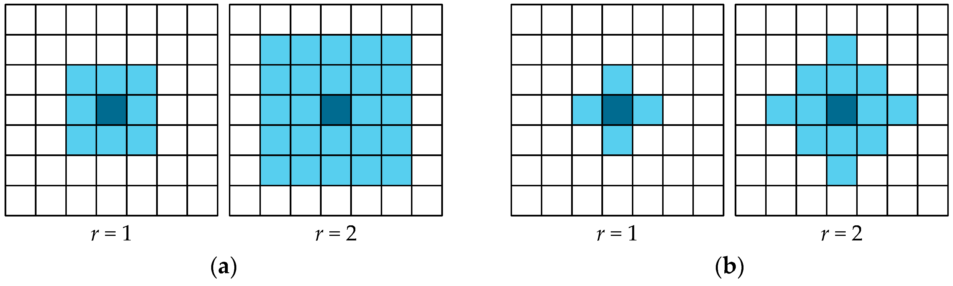
The local transition function is applied to all lattice cells during the evolution of a cellular automaton simultaneously. This function can be defined analytically or as a set of parallel substitutions. The cell neighborhood is regarded as a set of lattice cells, the current states of which will affect the state of a given cell in the next moment of time. A cell for which the neighborhood is constructed is called the central cell. Every neighborhood pattern element is a vector of the relative indices defining the position of a single neighborhood cell relative to the central cell, i.e., , , , where r is an integer, usually with a small value. For example, for classic Moore or Von Neumann neighborhoods, r = 1.
Also, here we should note that the neighborhoods of that type have the property of geometrical symmetry towards the central cell, as can be seen in
Figure 1, and they are used in the experiments shown further down.
Consequently, during the update of every lattice cell state, the states of
k adjacent cells, whose position relative to the central cell is defined by the neighborhood pattern
Y, are taken to be σ function arguments [
14,
17,
18].
Using a cellular automaton with a finite-sized lattice seems more natural in applied problems. In such a case, the model of a cellular automaton can be defined as , where , , is a vector setting the lattice size. When accessing cells situated outside the lattice, their coordinates are resolved by , , which is called “wrap-around” in terms of cellular automata.
Let us give a new extension of classic cellular automaton model.
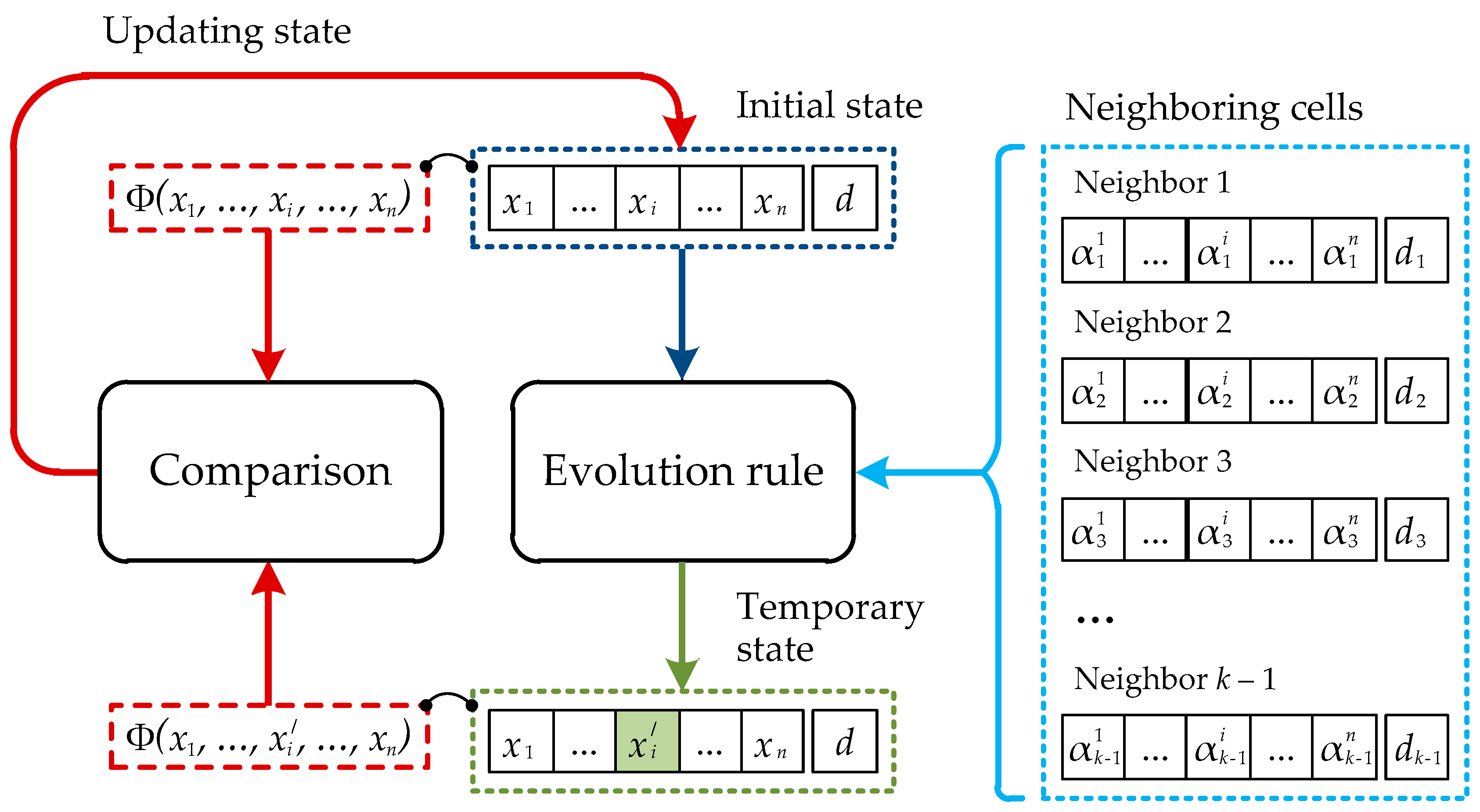
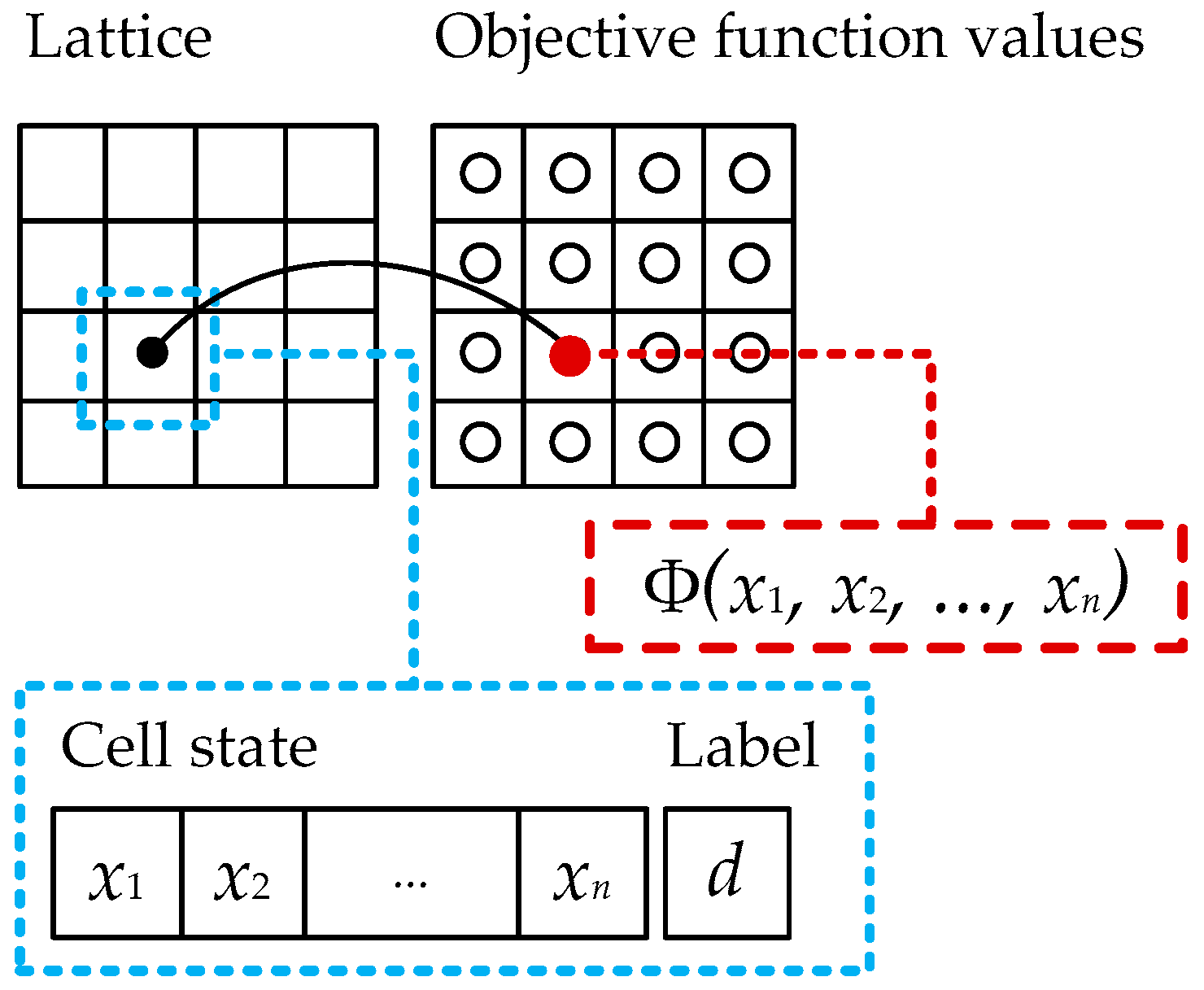
Definition 2. Let be a cellular automaton with an objective function, where , L, and Y correspond to analogical components of classic model; the set A is modified and looks like , where D is a set of labels; is a local transition function; is a cell marking-out rule; and is an objective function.
Every lattice cell of such a cellular automaton contains the real values vector (which is regarded as an element of an objective function domain) and an integer label which defines the quality of a solution contained in the x vector in terms of its proximity to the best solution acquired at this step of a cellular automaton evolution. Let us call the x vector the state of a cell. The local transition function can be defined only analytically, because it operates with real instead integer values.
The main features of the introduced model are shown in
Figure 2. The lattice of the cellular automaton is supplemented with the separate plane containing values of an objective function for all cells.
Figure 3 shows the general scheme, according to which the state of a separate cell of the lattice of the cellular automaton with an objective function is renovated.
Updating of the cell state is carried out under control of the objective function. Thus, separate measurements of the x vector, contained in the cell, vary sequentially and independently from each other. The new value of the i-th element of the x vector is calculated according to the chosen rule of evolution on the basis of the corresponding values contained in the neighboring cells belonging to the neighborhood of the given cell.
The most important element of the presented scheme is the rule of the cellular automaton development. Effectiveness of the offered model for solving the optimization problem depends on this rule. The rules of development introduced by us are presented in the following section of the given article.
2.3. The Procedure of the Cellular Automaton with an Objective Function Evolvement
For clarity, assume from now on that the evolution of a cellular automaton is pointed on the minimization of the objective function. The set of labels
D is understood to consist of the two elements
and the marking-out rule for labeling cells
U is defined as
where
and
are the minimum and the maximum of the objective function under the current step of the cellular automaton evolution respectively; and
is a preassigned parameter of the principle of cells labeling.
By means of the given rule the separate solutions contained in cells, divide into “bad” and “good” depending on their proximity to the best current solution. The extent of this proximity is defined by parameter μ. The label with the meaning “1” corresponds to the cells containing “good” solutions, and the label with the meaning “0” corresponds to the cells containing “bad” solutions. Cells with the label 0 are excluded from the neighborhood of the central cell in the following step of the evolution of the cellular automaton, or they are treated in a special way depending on a certain rule of evolution.
Let us define the two types of local transition functions of a cellular automaton with an objective function. We will use the following notation.
is the search space.
is the state of the central neighborhood cell in relation to which the local transition function is being recorded, and is its label. The cell indexing from now on will be dropped for brevity.
is the state of the neighborhood cells, recorded in the corresponding neighborhood pattern order, and are the labels. The central cell also belongs to its neighborhood, thus for certain p, , and .
is the real vector differing from x with j-th element value.
Then the local transition function of the first type is defined as
where
and
,
,
,
,
Updating of cell states of the cellular automaton by means of the presented function of transition is carried out as follows. Every element of the vector located in the cell is updated independently from the other elements. The new value of the i-th element of a vector is calculated by neighborhood averaging. The modification is accepted only in the case that it has led to improvement of the solution contained in the cell. Otherwise, the value of the i-th element of the vector contained in the cell remains without modifications.
The new state of the central cell forms only on the part of the neighborhood cells which contains “good” solutions. The function W, in its turn, excludes from the computation the elements of the neighborhood cells which are significantly remote from the corresponding central cell elements in the search space. That is determined by the parameter ω.
Thus, the marking-out rule introduced earlier defines which cells of the neighborhood take part in the formation of a new state of the central cell and which do not. Function W serves for additional marking-out of “good” cells on separate measurements. If the value of the i-th element of the neighborhood cell that has been labelled as “good” is considerably distant from the value of the i-th element of the central cell, the given “good” cell does not participate in formation of the new value of the i-th element of the central cell.
The local transition function of the second type is defined as
where
and
,
,
.
The increment function ∆ is defined as
where
r is a random natural number, and
s is a random real number from the interval [0, 1].
As in the previous case, all elements of the vector contained in a cell are processed independently from each other. The modification of the i-th element is accepted only in the event that it has led to improvement of the solution contained in the cell. For calculation of a new value of the i-th element of the vector contained in the central neighborhood cell, the increment function Δ is used. If the regenerated cell is “bad”, the value Δ for the i-th measurement is calculated by the modified formula of the root-mean-square error where the i-th element of the central cell is taken instead of an average value. It allows us to stay away from the current “bad” solution contained in the cell. If the updated cell is “good”, a small random value is taken as Δ. It allows us to investigate the neighboring area in the search space.
2.4. The Suggested Algorithm of Continuous Optimization on the Basis of the Cellular Automaton with an Objective Function
The general approach to finding the optimum of an objective function by means of the cellular-automata model is the following: in accordance with the given model, the parameters of the objective cellular automaton, and the number of development steps are set; the crosshatch of the cellular automaton is filled with random values from the search space; the development of the cellular automaton is launched within the set number of steps; the condition of one of the cells from the total configuration of the crosshatch, which is the best solution, is taken to be the required optimum point.
This paper studied the dynamics of the cellular automaton with an objective function, which was based on the principles of the development set by the expressions (2) and (3), in order to find out its ability to converge to the optimum of the set objective function. The standard test functions of many parameters were chosen as objective functions. Their list is given in
Table 1. All the experiments were run using two-dimensional cellular automaton.
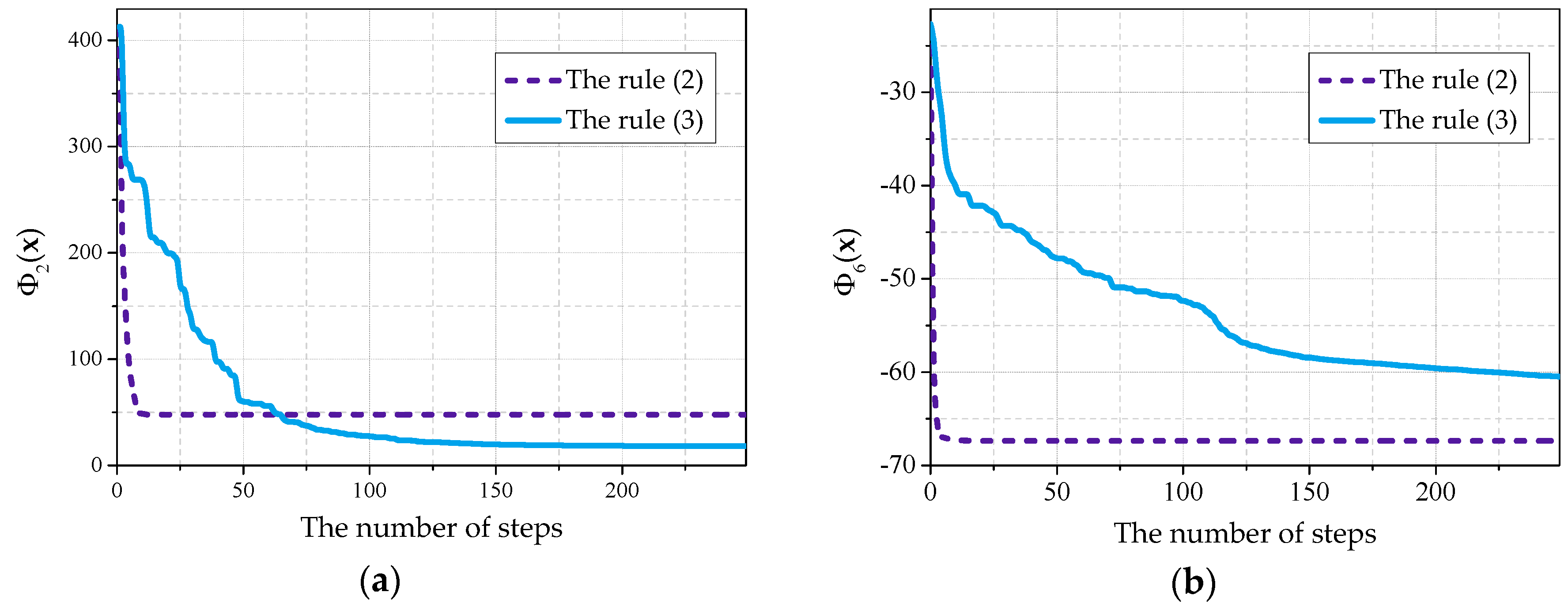
As a result, it was discovered that, when choosing the rule of the development on the basis of increment (3), the dynamics of the cellular automaton in the majority of cases has better convergence in comparison with the rule on the basis of averaging (2). However, the usage of these rules individually allowed us to find the optimum values only of some testing objective functions from the plurality of the examined ones. Using the rule (2) we were able to get the optimum of the function with the error not more than 0.03, and using the rule (3) it was possible to get the optima of the functions , , and with the error not more than 0.05.
In
Figure 4a, the graph presenting the process of the optimization of the
is given. Each graph presented in the given article has been received by averaging the results of 30 experiments.
It can be seen that, when using the rule (2) during the first 10 steps, fast movement to the optimum value side is observed, but after that the development stops. When using the rule (3) noticeable movement to optimum value side is observed in duration of the first 100–200 steps. However, the rule (2) differs by a prominently faster speed of convergence during the first effective steps of the cellular automaton development.
A similar picture was observed for the majority of objective functions. Nevertheless, in some cases a cellular automaton was able to advance to the optimum side noticeably farther using the rule (2), rather than using the rule (3), as it is shown in
Figure 4b using
as an example.
Due to this, a continuous optimization algorithm, being a general result of this paper, was based on the composition of suggested rules of evolvement of a cellular automaton with an objective function. This algorithm, formulated for a two-dimensional cellular automaton, is represented below.
Input:
a vector denoting sizes of a cellular automaton lattice, ; a neighborhood pattern Y; cell marking-out rule parameter μ; a ratio of an acceptable remoteness of neighborhood cell states from corresponding central cell elements ω; an objective function of m variables , the optimum(minimum) of which has to be found; search space borders ; a number of cellular automaton evolvement steps T.
Output:
a vector
, defining a point of the optimum being sought for.
- Step 1.
Fill the states of all cellular automaton lattice cells with random values from .
- Step 2.
Calculate an objective function value for each lattice cell, storing these values in a matrix.
- Step 3.
Find a minimal element in the M matrix. Write this element value to and its coordinates to .
- Step 4.
Find the maximum element in the M matrix. Write this element value to .
- Step 5.
Calculate the label for each cell according to the rule (1).
- Step 6.
For
t from 1 to
T do:
- Step 6.1.
For
i from 1 to 3 do:
- Step 6.1.1.
Update every lattice cell state according to the evolvement rule (2) and neighborhood pattern Y.
- Step 6.1.2.
Update the M matrix, , , and .
- Step 6.1.3.
Update every cell label according to the rule (1).
- Step 6.2.
Update every cell state according to the evolvement rule (3) and neighborhood pattern Y.
- Step 6.3.
Update the M matrix, , , and .
- Step 6.4.
Update every cell label according to the rule (1).
- Step 7.
Return state of the cell with coordinates as the x vector and finish the algorithm.
3. Experiments
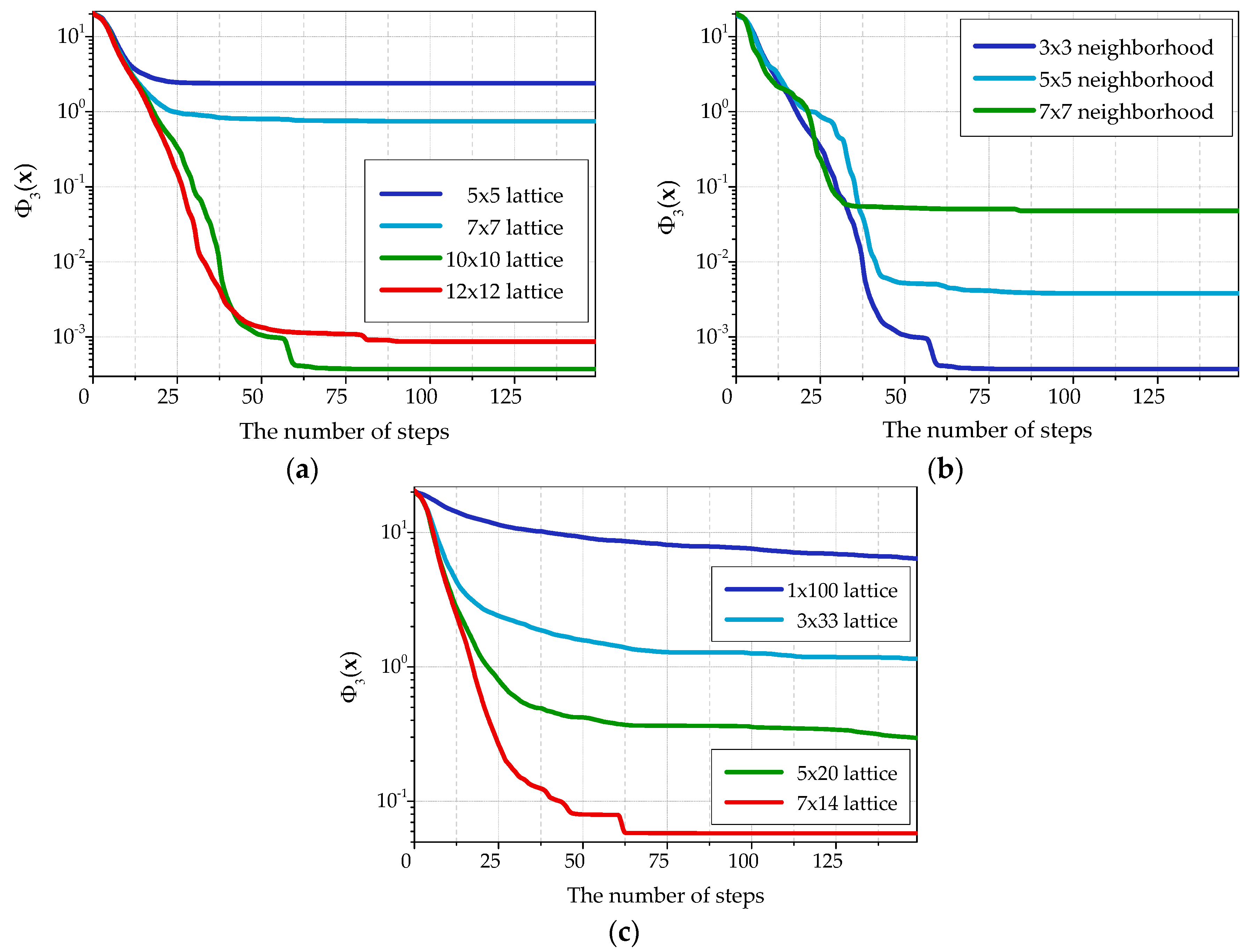
Figure 5 represents convergence plots built for the
function with different optimization algorithm parameters. Using other objective functions gave similar plots. The best results are obtained for the cellular automaton with 10 × 10 cell lattice and Moore neighborhood with single-unit radius (3 × 3 cells). Further increase of the lattice and Moore neighborhood sizes leads to convergence deterioration.
Notice that not only the number of cells in a lattice of the cellular automaton influences the quality of optimization, but also the lattice form. The accuracy of the received solutions increases at the approach of the lattice form to a square as it can be seen in
Figure 5c. Besides, a one-dimensional cellular automaton with the lattice of 1 × 100 cells shows the worst result.
The main analog for the algorithm being described is the CLA-DE algorithm represented in [
16], because among all the algorithms being considered it keeps the properties of cellular automaton model to the fullest extent. That algorithm is based on the dynamics of a cellular automaton-designed system, every cell of which contains a set of learned automata responsible for the changes of separate variables of an objective function in the search space.
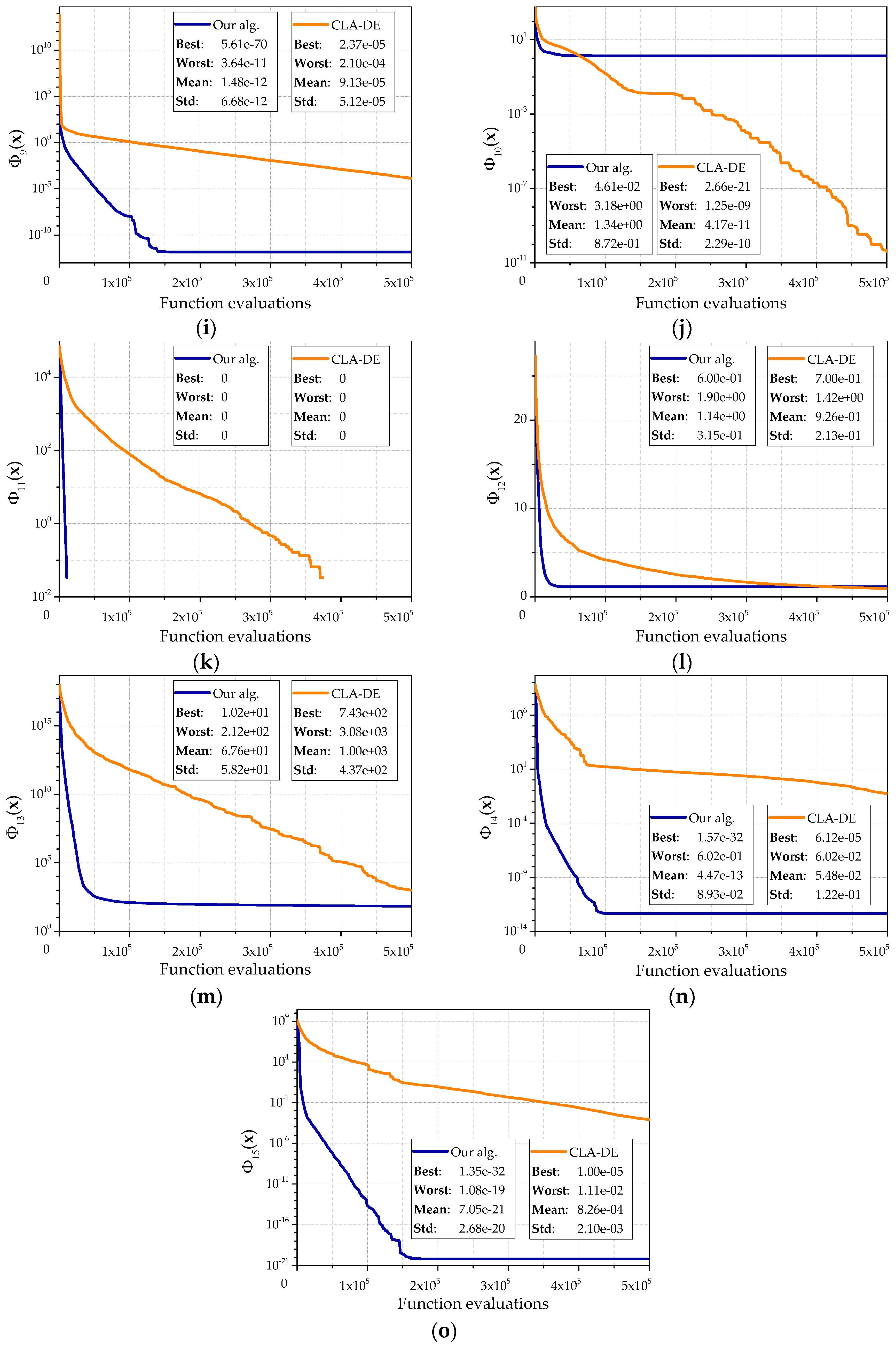
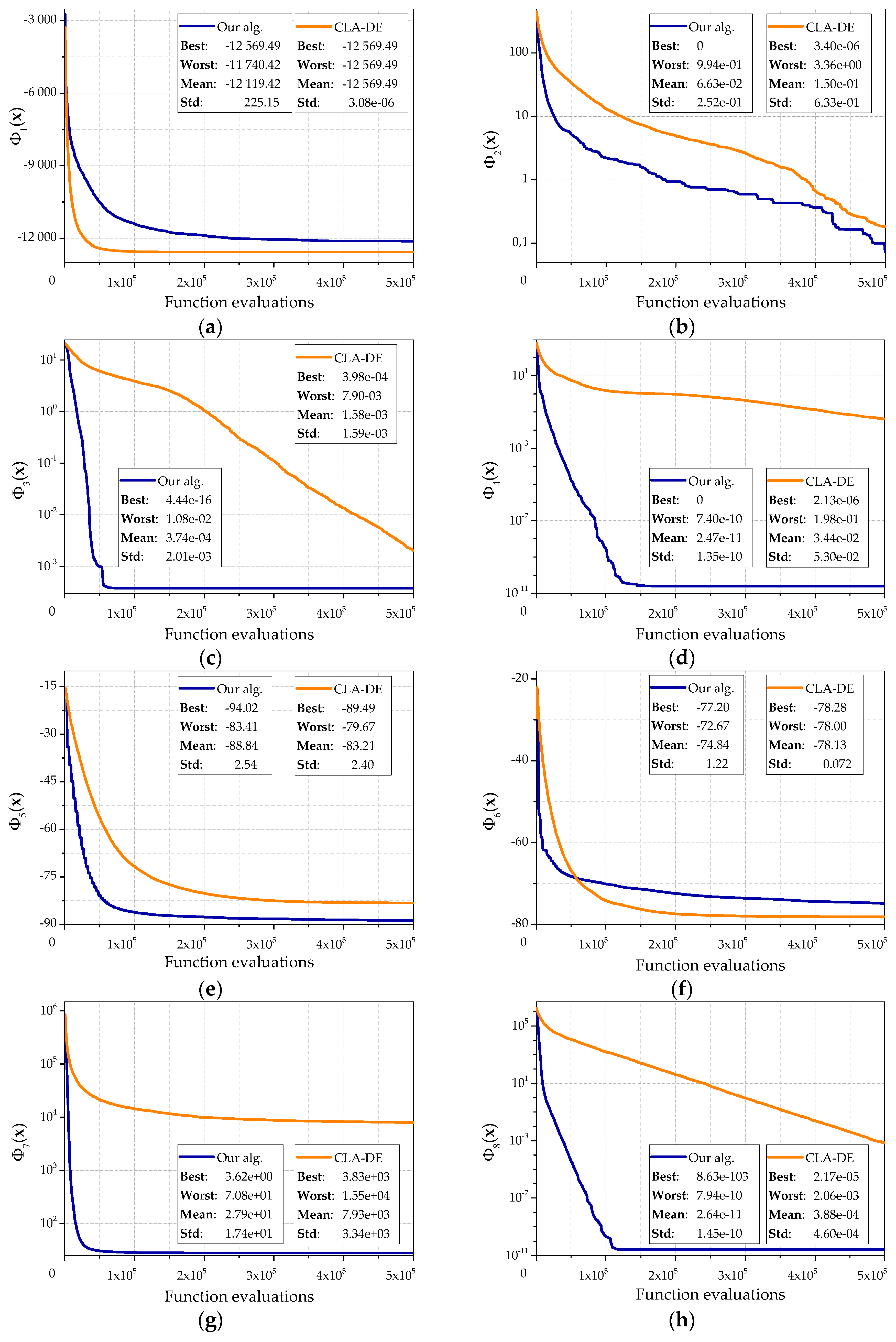
Figure 6 denotes the results of the corresponding experiments for 15 test objective functions. The following algorithm parameter values were used:
L = (10, 10),
,
,
,
.
Since an amount of calculation for the objective function on first step of the learning cellular automaton and an amount of calculation for the objective function on the first step of the cellular automaton are different, the average dependence of the best found value and the amount of calculation of the objective function for 30 runs is shown. During each run, 500,000 function evaluations were performed. Each graph shows the best result, the worst result and the standard deviation.
The character of these graphs allows us to make the following conclusions. Our algorithm has a higher speed of convergence than the CLA-DE. It quickly reaches a sufficiently accurate approximation to the optimum, which is shown by a bigger angle of curves. Generally, the proposed algorithm is better than CLA-DE on both the average and the best values. CLA-DE is better only in some cases, for example, on the objective function . This can be explained by getting into local optimum, which is abundantly presented in the function . A similar situation is observed for the function . It should be noted that the CLA-DE gets into local optimums less frequently. The lack of horizontal sections on the curves that sometimes appear in our algorithm also shows it. Experiments showed that in some cases CLA-DE is able to continue to move toward the optimum longer than our algorithm. This property is clearly seen, for example, on functions , , . However, this increase of accuracy can be achieved only by increasing the number of calculations.
This observation is also confirmed by experiments with the objective functions and , which are the Rosenbrock functions with dimension 30 and 10, respectively. For the function our algorithm returns a value close to the optimum. CLA-DE significantly does not achieve the optimum and shows the worst result. However, in most of the experiments for the function our algorithm also quickly comes to a value close to the optimum, and stops the evolution, while CLA-DE continues to move toward the optimum. Our algorithm still shows a higher speed of convergence on the first iterations.
On the example of objective function , CLA-DE is also ahead of our algorithm, but only by average result by virtue of smaller spread in the values received in separate experiments. CLA-DE is behind our algorithm compared to the best result which has been received for the given function. Besides, lower speed of CLA-DE convergence leads to the fact that the advantage of the average value is shown only after 400,000 function evaluations.
For an estimation of significance of the received results we will use the following nonparametric statistical tests intended for pairwise comparison algorithms: Sign test and Wilcoxon test [
19].
As a value characterising productivity of algorithms we will use the error obtained for each one over the 15 benchmark functions considered.
Table 2 shows the best and average values of this value which were received during a various number of function evaluations: 50,000 and 500,000. Statistical comparison of the results obtained by means of two considered algorithms for a small number of function evaluations will serve for refinement of the above mentioned observations.
The results of the application of Sign test and Wilcoxon test to the given data sets are shown in
Table 3 and
Table 4.
Table 3 shows the number of wins and losses of our algorithm in four considered cases, and the level of significance for each case is defined. Identical results are divided equally between both algorithms.
We can see that, for 50,000 function evaluations, our algorithm shows significant improvement over CLA-DE with a level of significance α = 0.05 both in the best and in average results. For 500,000 function evaluations our algorithm shows significant improvement over CLA-DE with the level of significance α = 0.1 in the best result and α = 0.05 in the average result.
Sign test is an elementary statistical test allowing one to evaluate the advantage of one algorithm over another with a series of experiments. However, it considers only the part of experiments in which the given algorithm showed the best result. Wilcoxon test is a stronger test as it also considers the difference in productivity for separate experiments.
We can see that, in three out of four cases, the Wilcoxon test confirms the considerable advantage of our algorithm over the CLA-DE algorithm. Our algorithm leaves CLA-DE considerably behind at a small number of function evaluations, both by average result, and by the best result. At a higher number of function evaluations our algorithm also advances CLA-DE by the best result, but for an average result it is not possible to disprove the null hypothesis.
It is connected to a wider dispersion of output values which is characteristic for our algorithm. At the same time, its ability to quickly obtain the values close to optimum, advancing the algorithm-competitor, is proved by the Wilcoxon test for a small number of function evaluations.
Thus, the conclusions made earlier at the analysis of the graphs in
Figure 6 are proved by statistical tests.
Earlier during the literature review other examples of use of cellular automata in problems of continuous optimization except CLA-DE were also considered. However, when analyzing corresponding algorithms, we determined that cellular automata are applied in these algorithm mainly indirectly. The given algorithms represent modifications of the known metaheuristics in which the cellular-automatic principle of local interactions is involved, but evolution of the cellular automaton is not defined. The CLA-DE algorithm considered by us as the main analog is possible to define as an exception. However, a cellular automaton is not exactly used but a set of trained automata united in a lattice. Also hybridization with differential evolution takes place.
Having compared the offered algorithm with CLA-DE, we showed that cellular automata can be used for the solution of problems of optimization not only as an auxiliary device but also as the basic computing model. Now we will compare our algorithm with some other metaheuristics that were considered earlier during the literature review: the artificial fish swarm algorithm based on cellular learning automata (AFSA-CLA) [
15] and the evolutionary membrane algorithm (EMA) [
13].
The results of additional comparison are given in
Table 5. The table shows the best result of each algorithm. We have carried out the given comparison with metaheuristics of those authors who presented the results of computing experiments with standard test functions from ones given in
Table 1. To provide equal conditions with the experiments described in the papers [
13,
15], the values given in the table were obtained after 300,000 function evaluations. A dash in a cell means that, for the given function, experimental data is absent.
Our algorithm shows the best result on the functions , , , –. AFSA-CLA shows the best result on the functions and . On the function and our algorithm and AFSA-CLA return the real optimum. EMA is better than our algorithm on the functions , but worse than AFSA-CLA.
The algorithm AFSA-CLA has a high performance because it is based on metaheuristics, which is effective in itself. Also, a learning cellular automaton improves these metaheuristics. This leads to higher performance than when a learning cellular automaton is used separately for optimization like it occurs in CLA-DE. AFSA-CLA is significantly ahead of our algorithm only on the function , in all other cases both algorithms show similar results. At the same time, our algorithm can achieve real optimum in two cases, but AFSA-CLA only in one case.
The algorithm EMA shows the worst results in terms of accuracy. However, according to [
13], this algorithm has a high speed of convergence and allows one to obtain acceptable values for a relatively small number of function evaluations. In this case, for the function
an error is negligible for all three algorithms, which allows us to consider that the results are equivalent.
The results of paired comparison of our algorithm with AFSA-CLA and EMA algorithms by means of statistical tests are shown in
Table 6. Initial data were calculated on the basis of the values given in
Table 1 and
Table 5.
When comparing with the AFSA-CLA algorithm, our algorithm is the winner in two cases out of six and in two cases the results coincide. This does not allow to disprove a null hypothesis and to establish the significant advantage of one algorithm over another. However, mainly it is connected to insufficient amount of experimental data for AFSA-CLA.
In turn, comparison with EMA shows that our algorithm considerably surpasses EMA with the significance level of α < 0.1.
Therefore, the algorithm suggested by us on the basis of the cellular automaton with an objective function shows more acceptable results in comparison with others metaheuristics.
4. Conclusions
The main objective of our research consisted in showing applicability of cellular automata for the solution of the problem of continuous optimization. The given mathematical apparatus has been applied in optimization problems for a long time. However, the analysis of known algorithms showed that cellular automata are mainly used as an auxiliary computing model. We want to show the possibility of direct application of cellular automata for optimization of arbitrary functions. For this purpose, we introduce the concept of the cellular automaton with an objective function, which is a modification of the classical cellular automaton. The introduced cellular-automata model has the following features:
The objective function is included in the model.
Each cell of the array contains the vector real value which is considered to be the element of function domain of the objective function .
The development of the cellular automaton is organized in such a way that, while renovating the state of each cell of the array, its new state will be closer to the optimum.
In this paper, two rules of cellular automaton with an objective function development are introduced, and properties of their convergence are analyzed.
On the basis of the described model with the usage of the two introduced rules, we formulated a new algorithm of continuous optimization, which belongs to the stochastic algorithm in connection to the usage of random values in development of the cellular automaton.
The conducted benchmarks showed the similarity of the effectiveness between the suggested algorithm and the analogs. The usage of the cellular automaton with the array 10 × 10 cells with Moore neighborhood 3 × 3, having the property of geometrical symmetry, has led to the top results.
The advantage of the developed algorithm is the convergence of fast speed during the first steps of the computation. This advantage lets us recommend the algorithm for use in real time data problems, where the speed of getting a solution closer to the optimum is more important than accuracy.
The goal of future research will be the development of the suggested approach, the research of new rules of the cellular automaton with an objective function development that are different from these being considered in this paper, and also the synthesis of new algorithms of continuous optimization on the basis of composition of the given rules.


 ,
, 


