Linear Weingarten Helicoidal Surfaces in Isotropic Space

Abstract

In the present paper, we study helicoidal surfaces in the three-dimensional isotropic space $I^3$ and construct helicoidal surfaces satisfying a linear equation in terms of the Gaussian curvature and the mean curvature of the surface.

1. Introduction

Introduced in 1861 [1], a Weingarten surface in the Euclidean three-dimensional space ${\mathbb{E}}^3$ is a surface M, whose mean curvature H and Gaussian curvature K satisfy a non-trivial relation $\Phi (H,K)=0$. Such a surface was introduced by Weingarten. The class of Weingarten surfaces is remarkably large, and it consists of intriguing surfaces in the Euclidean space: the constant mean curvature surfaces, the constant Gaussian curvature surfaces and all rotational surfaces.

As a special case of Weingarten surfaces, we consider that the Weingarten relation Φ is linear in its variables. That is, Φ satisfies the following relation

$$aH+bK=c$$

(1)

for a, b, and c are not all zero real numbers. Such a surface with the Equation (1) is said to be a linear Weingarten surface (briefly, LW-surface). Especially, in the case for $a=0$ or $b=0$ in (1), LW-surfaces are Weingarten surfaces either with a constant Gaussian curvature or with a constant mean curvature, respectively. The classification of Weingarten surfaces and linear Weingarten surfaces in the general case is almost completely open today. Several geometers are studying Weingarten surfaces and linear Weingarten surfaces in the ambient spaces, and many interesting results can be found in [2,3,4,5,6,7,8,9,10,11,12,13,14] etc.

2. Preliminaries

The three-dimensional isotropic space $I^3$ was introduced by Strubecker in the 1940s, and it is based on the following group $G_6$ of affine transformations $(x,y,z)\to (\overline{x},\overline{y},\overline{z})$ in ${\mathbb{R}}^3$,

$$\begin{array}{cc}\hfill \overline{x}& =a+xcos\varphi -ysin\varphi ,\hfill \\ \hfill \overline{y}& =b+xsin\varphi +ycos\varphi ,\hfill \\ \hfill \overline{z}& =c+c_{1}x+c_{2}y+z,\hfill \end{array}$$

where $a,b,c,c_1,c_2,\varphi \in \mathbb{R}$. Such affine transformations are called isotropic congruence transformations or isotropic motions of $I^3$ (cf. [15]). We see that isotropic motions appear as Euclidean motions (a translation and a rotation) in the projection onto the $xy$-plane; the result of this projection $P=(x,y,z)\to P^{\prime }=(x,y,0)$ is called "top view". Hence, an isotropic motion is composed of a Euclidean motion in the $xy$-plane and an affine shear transformation in the z-direction.

On the other hand, the isotropic distance of two points—$P=(x_1,y_1,z_1)$ and $Q=(x_2,y_2,z_2)$—is defined as the Euclidean distance of the top views, i.e.,

$$d{(P,Q)}_i:=\sqrt{{(x_1-x_2)}^2+{(y_1-y_2)}^2}.$$

(2)

In fact, two points $(x,y,z_i)$$(i=1,2)$ with the same top views have the isotropic distance of zero, called "parallel points". The isotropic metric (2) degenerates along z-parallel lines, called "isotropic lines". Isotropic angles between straight lines are measured as Euclidean angles in the top view. There are two types of planes in $I^3$: isotropic planes are planes parallel to the z-direction, and otherwise they are non-isotropic planes.

Let $\mathbf{x}=(x_1,y_1,z_1)$ and $\mathbf{y}=(x_2,y_2,z_2)$ be vectors in $I^3$. The isotropic inner product of $\mathbf{x}$ and $\mathbf{y}$ is defined by

$${\langle \mathbf{x},\mathbf{y}\rangle }_i=\left\{\begin{array}{cc}{z}_1{z}_2,\hfill & \mathrm{if}{x}_i=0\mathrm{and}{y}_i=0\hfill \\ x_1{x}_2+y_1{y}_2,\hfill & \mathrm{if}\mathrm{otherwise}.\hfill \end{array}\right.$$

(3)

We call a vector of the form $\mathbf{x}=(0,0,z)$ in $I^3$ an "isotropic vector", and a "non-isotropic vector" otherwise.

Consider a $C^r$-surface M, $r\ge 1$, in $I^3$ parameterized by

$$X(u,v)=(x(u,v),y(u,v),z(u,v)).$$

A surface M immersed in $I^3$ is called admissible if it has no isotropic tangent planes. We restrict our framework to admissible regular surfaces.

For such a surface, the coefficients $g_{ij}$ $(i,j=1,2)$ of its first fundamental form are given by

$$g_{11}={\langle X_u,X_u\rangle }_i,g_{12}={\langle X_u,X_v\rangle }_i,g_{22}={\langle X_v,X_v\rangle }_i,$$

where $X_u=\frac{\partial X}{\partial u}$ and $X_v=\frac{\partial X}{\partial v}.$ On the other hand, the unit normal vector of M is always the isotropic vector $(0,0,1)$ since it is perpendicular to all tangent vectors to M. The coefficients $h_{ij}$$(i,j=1,2)$ of the second fundamental form of M are calculated with respect to the normal vector of M and they are given by

$$h_{11}=\frac{det(X_{uu}{X}_u{X}_v)}{\sqrt{det(g_{ij})}},h_{12}=\frac{det(X_{uv}{X}_u{X}_v)}{\sqrt{det(g_{ij})}},h_{22}=\frac{det(X_{vv}{X}_u{X}_v)}{\sqrt{det(g_{ij})}}.$$

The isotropic Gaussian curvature K and the isotropic mean curvature H are defined by

$$K=\frac{det(h_{ij})}{det(g_{ij})},H=\frac{g_{11}{h}_{22}-2g_{12}{h}_{12}+g_{22}{h}_{11}}{2det(g_{ij})}.$$

(4)

The surface M is said to be isotropic flat (resp. isotropic minimal ) if K (resp.H) vanishes (cf. [16]).

An isotropic three-dimensional space, which is one of the Cayley-Klein spaces defined from the projective three-dimensional spaces, is obtained from the Euclidean space by substituting the usual Euclidean distance with the isotropic distance. The work of surfaces with special properties in an isotropic three-dimensional space has important applications in several applied sciences, e.g., computer science, image processing, architectural design and microeconomics, see [15].

In this paper, we study helicoidal surfaces in an isotropic three-dimensional space. The surfaces are invariant by an isotropic motion and a translation. The main purpose of this paper is to construct helicoidal surfaces in an isotropic three-dimensional space satisfying the linear Weingarten relation (1).

3. Main Results

In this section, we completely construct linear Weingarten helicoidal surfaces in an isotropic three-dimensional space $I^3$ in terms of the Gaussian curvature and the mean curvature of the surface. To define helicoidal surfaces in an isotropic space $I^3$, we consider a curve γ lying in the isotropic $xz$-plane or $yz$-plane without loss of generality. Then, the profile curve γ is parameterized as

$$\gamma (u)=(f(u),0,g(u))\mathrm{or}\gamma (u)=(0,f(u),g(u)),$$

where f and g are smooth functions. Together with the Euclidean rotations in the isotropic space $I^3$, given by the normal form (in affine coordinates)

$$\left\{\begin{array}{c}\overline{x}=xcos\varphi -ysin\varphi ,\hfill \\ \overline{y}=xsin\varphi +ycos\varphi ,\varphi \in \mathbb{R},\hfill \\ \overline{z}=z,\hfill \end{array}\right.$$

and a translation, a helicoidal surface M in $I^3$ can be parameterized by

$$\begin{array}{cc}\hfill X(u,v)& =\left(\begin{array}{ccc}cosv& -sinv& 0\\ sinv& cosv& 0\\ 0& 0& 1\end{array}\right)\left(\begin{array}{c}f(u)\\ 0\\ g(u)\end{array}\right)+v\left(\begin{array}{c}0\\ 0\\ h\end{array}\right)\hfill \\ & =\left(f(u)cosv,f(u)sinv,g(u)+hv\right)\hfill \end{array}$$

(5)

or

$$\begin{array}{cc}\hfill X(u,v)& =\left(\begin{array}{ccc}cosv& -sinv& 0\\ sinv& cosv& 0\\ 0& 0& 1\end{array}\right)\left(\begin{array}{c}0\\ f(u)\\ g(u)\end{array}\right)+v\left(\begin{array}{c}0\\ 0\\ h\end{array}\right)\hfill \\ & =\left(-f(u)sinv,f(u)cosv,g(u)+hv\right),\hfill \end{array}$$

(6)

where $h\in \mathbb{R}$. Then, the helicoidal surfaces given by (5) and (6) are locally isometric. Our study is concentrated on the helicoidal surface given by (5).

Suppose that a profile curve $\gamma (u)=(f(u),0,g(u))$ is a unit speed curve. Then we can take $f(u)=u$. Thus, a helicoidal surface in $I^3$ is parameterized by

$$X(u,v)=(ucosv,usinv,g(u)+hv),$$

where $u\in \left(0,\infty \right)$ and $v\in \mathbb{R}$. In this case, the components of the first fundamental form of M are given by

$$g_{11}=1,g_{12}=0,g_{22}=u^2,$$

and the components of the second fundamental form of M are

$$h_{11}=g^{\prime \prime },h_{12}=-\frac{h}{u},h_{22}=u{g}^{\prime }.$$

Since M is a non-degenerate surface, $u\ne 0$. From now on, $"{}^{\prime }"$ means the partial derivative with respect to the parameter u unless mentioned. Thus, the Gaussian curvature K and the mean curvature H of M are given by

$$K=\frac{u^3{g}^{\prime }{g}^{\prime \prime }-h^2}{u^4},$$

(7)

and

$$H=\frac{g^{\prime }}{u}+g^{\prime \prime }.$$

(8)

Let M be a linear Weingarten helicoidal surface in an isotropic three-dimensional space satisfying the condition $aH+bK=c,$ where $a,b,c\in \mathbb{R}$. It is well-known that surfaces with a constant Gaussian curvature $(b=0)$ and a constant mean curvature $(a=0)$ are trivial solutions of linear Weingarten surfaces. On the other hand, Aydin [17] classified all helicoidal surfaces in an isotropic three-dimensional space with a constant Gaussian curvature and a constant mean curvature.

To obtain non-trivial solutions of linear Weingarten surfaces, we consider

$$aH+K=b,a,b,\in \mathbb{R},a\ne 0.$$

(9)

Now, we discuss a helicoidal surface satisfying (9). Put

$$A=u{g}^{\prime }.$$

(10)

Then (7) and (8) can be rewritten as the form

$$K=\frac{1}{u}{\left(\frac{A^2}{2u^2}+\frac{h^2}{2u^2}\right)}^{\prime },$$

(11)

$$H=\frac{1}{u}{A}^{\prime },$$

(12)

respectively.

Suppose that M is a non-trivial linear Weingarten surface. Then from (11) and (12), Equation (9) implies

$$a\frac{1}{u}{A}^{\prime }+\frac{1}{u}{\left(\frac{A^2}{2u^2}+\frac{h^2}{2u^2}\right)}^{\prime }=b.$$

After solving the ordinary differential equation, we obtain

$$A^2+2a{u}^{2}A+h^2-b{u}^4-2c{u}^2=0$$

for some constant c. Thus, we have

$$A=-a{u}^2\pm \sqrt{(a^2+b)u^4+2c{u}^2-h^2}.$$

(13)

By combining (10) and (13), one yields

$$g(u)=-\frac{1}{2}a{u}^2\pm \int \frac{1}{u}\sqrt{(a^2+b)u^4+2c{u}^2-h^2}du+d,d\in \mathbb{R}.$$

(14)

In (14), there are two functions for g. Without loss of generality, we take the sign + in the above expression (the reasoning is analogous with the choice−).

On the other hand, we can calculate the integral term in (14) with the help of the result in (see [17], page 7), it follows that

$$\begin{array}{cc}\hfill g(u)& =-\frac{1}{2}a{u}^2+\frac{1}{2}\sqrt{(a^2+b)u^4+2c{u}^2-h^2}-\frac{h}{2}{tan}^{-1}\left(\frac{c{u}^2-h^2}{h\sqrt{(a^2+b)u^4+2c{u}^2-h^2}}\right)\hfill \\ & +\frac{c}{2\sqrt{a^2+b}}ln\left|2c+2(a^2+b)u^2+2\sqrt{a^2+b}\sqrt{(a^2+b)u^4+2c{u}^2-h^2}\right|+d.\hfill \end{array}$$

(15)

Consequently, we have proven the following result.

Theorem 1.

Let M be a helicoidal surface in an isotropic three-dimensional space parameterized by

$$X(u,v)=(ucosv,usinv,g(u)+hv).$$

If M is a non-trivial linear Weingarten surface satisfying $aH+K=b$ with $a,b\in \mathbb{R},a\ne 0$, then the function g is given by (15).

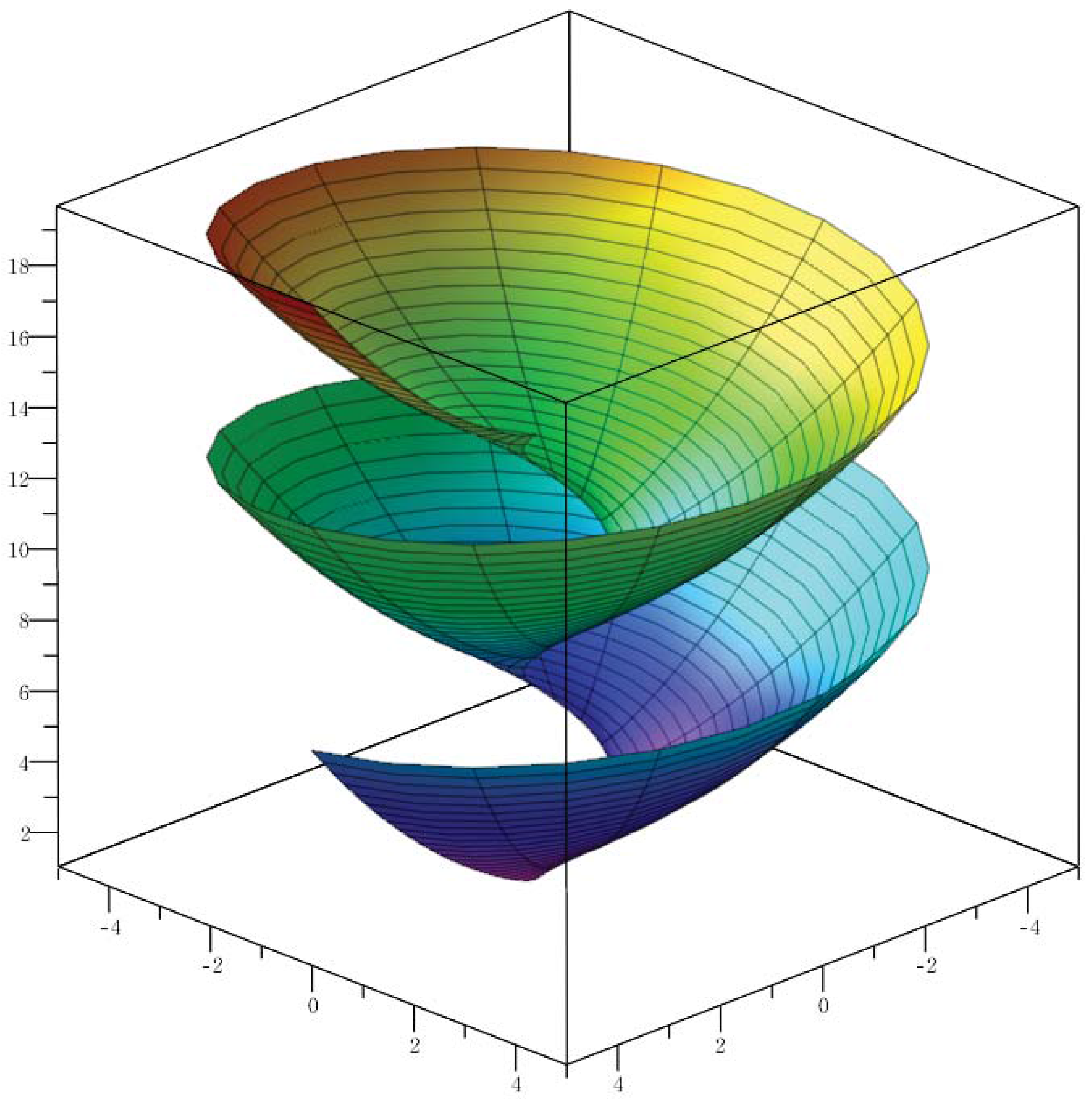
Remark 1.

If $a=0$ in (9) (i.e., K is constant.), Theorem 1 is the same as Theorem 3.1 in [17].

Remark 2.

For $a=b=c=1$ and $h=1$ in (15), we have the LW helicoidal surface (see Figure 1).

In the special case that M is a rotational surface (i.e., $h=0$) in an isotropic three-dimensional space, we have the same result with Theorem 3.2 in Ö$\breve{\mathrm{g}}$renmiş’s work as follows:

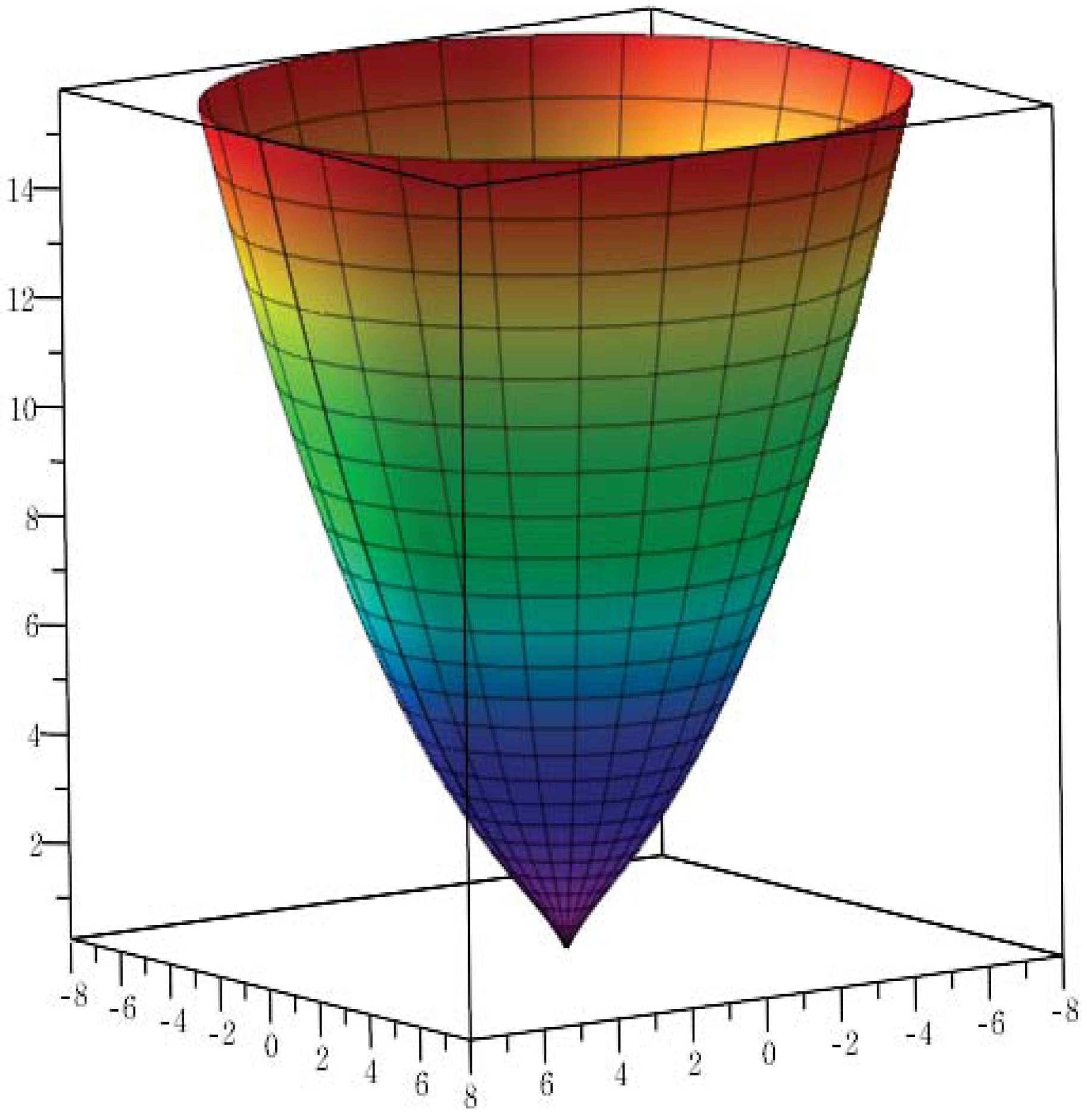
Corollary 1.

[18] Let M be a rotational surface in an isotropic three-dimensional space parameterized by

$$X(u,v)=(ucosv,usinv,g(u)).$$

If M is a non-trivial linear Weingarten surface satisfying $aH+K=b$ with $a,b\in \mathbb{R},a\ne 0$, then the function g is given by

$$\begin{array}{cc}\hfill g(u)& =-\frac{1}{2}a{u}^2+\frac{1}{2}u\sqrt{(a^2+b)u^2+2c}\hfill \\ & +\frac{c}{2\sqrt{a^2+b}}ln\left|2c+2(a^2+b)u^2+2u\sqrt{a^2+b}\sqrt{(a^2+b)u^2+2c}\right|+d.\hfill \end{array}$$

Remark 3.

For $a=b=c=1$ in Corollary 2, we have the LW rotational surface (see Figure 2).