1. Introduction
Generally speaking, integrable equations are related to linear equations either by a classical Darboux transformation (c-integrable) or an inverse scattering transform (s-integrable) [
1]. There are two main pathways that use Lie symmetry groups to identify integrable equations. The first is the detection of extended symmetries of order three or higher. Unlike first-order contact symmetries and their equivalent second-order “vertical” symmetries, higher-order symmetry transformations cannot be closed at some finite order [
2]. While the very demanding condition of existence of a third-order symmetry is still not a sufficient condition for integrability, it is a useful and practical sieve. Known examples of equations with higher-order symmetries, are often members of a hierarchy of commuting integrable symmetries at successively higher orders, connected by a symmetry recursion operator (e.g., [
3,
4]). This approach has the advantage that it may reveal equations that are integrable in either sense of being s-integrable or c-integrable.
The second pathway involves detection of a general solution of a linear equation within the Lie point symmetry group or the Lie group of potential symmetries of a Darboux integrable equation. That method has the advantage of an inbuilt algorithm for finding the linearising transformation [
5,
6].
Classification of integrable scalar evolution equations in one space dimension, is well understood [
7]. An inverse scattering transform has been found for some systems of N-waves in two and three dimensions [
8]. However, it remains challenging to apply symmetry methods to classify integrable
systems of parabolic evolution equations in
more than one space dimension. As a test bed for such methods, in the following sections, some directly integrable vector-valued extensions of Burgers’ scalar equation in three spatial dimensions, are considered.
The only source of nonlinearity in the Navier–Stokes momentum transport equation is the deceptively innocuous-looking quadratic inertial term within the convective time derivative
Naturally, one seeks to gain insight from simplified transport models that at least retain this nonlinear term. For example, in gas dynamics it is common to assume the inviscid first-order Euler equations [
9,
10]. In one space dimension, there is the integrable transport model, the Burgers equation
This equation resembles the momentum transport equation of incompressible Newtonian fluid but of course one-dimensional incompressible flow is trivial. Therefore solutions are considered with
non-zero. In this sense, Equation (
1) is often used as a prototype model for compressible gas dynamics, but with the shocks smoothed by the non-zero viscosity [
11,
12]. The equation has found direct applications also in other areas, such as sedimentation [
13] and soil-water transport [
14], in which
u represents a scalar concentration variable.
The one-dimensional Burgers equation has long been known to be exactly transformable to the classical linear heat diffusion equation by the Cole–Hopf transformation [
15,
16], previously given as an exercise in the text by Forsyth ([
17], p. 102, Ex. 3). However this linearisation applies to the three dimensional prototype transport equation only after an additional constraint is appended. The Cole–Hopf transformation was applied in [
18] to the three dimensional Burgers equation but necessarily with the additional constraint of irrotational flow. Matskevich [
19] investigated how the Cole–Hopf transformation could simplify the Burgers equation in invariant form adapted to flow on a pseudo-Riemannian manifold. The outcome was that on a manifold with constant non-zero Ricci curvature scalar, Burgers’ equation transforms to a reaction-diffusion equation for scalar Cole–Hopf potential
ψ, with linear diffusion term but nonlinear reaction term proportional to
. In
Section 2 here, the reverse question is easily answered, namely after specifying that the Cole–Hopf potential satisfies a general
linear or semi-linear second-order reaction-diffusion equation. What is the most general form of the integrable nonlinear vector equation that results from the Cole–Hopf transformation in the reverse direction ?
In fact any system of the following form is integrable:
where
and
are differentiable symmetric tensor-valued, vector-valued and scalar-valued functions respectively, and
is a non-zero constant. Here,
,
is the time coordinate,
:
are the space coordinates, repeated indices are summed and
is the alternating symbol that is
for even(odd) permutations
of
. The
n-dimensional version of Equation (2) (
) remains integrable when
is the gradient of some scalar potential, as shown in the next section. Unlike in one dimension, in higher dimensions it is more convenient to use index notation, especially when the coordinates are allowed to be non-Cartesian.
2. Extension of Cole–Hopf Transformation to n-Dimensions
Suppose that the scalar function
is a classical solution of the general linear second-order parabolic equation
with
, defined on a closed subset Ω of
. Define a velocity potential
ϕ by
is a generalisation of a scalar velocity potential, which as a consequence of Equation (
4), satisfies
Then
satisfies the generalised Burgers Equation (2). Note that under this transformation, the
-dependent terms cancel, so that this parameter does not appear in Equation (2). For this reason it is usually convenient to assume the homogeneous version of Equation (
4) with
. Note also that Equation (2) is sufficiently general to allow the diffusion term to be an isotropic kinematic viscosity coefficient multiplied by the Laplace-Beltrami operator for a Riemannian manifold, acting on
. That is the right hand side is
plus terms of order 1 and 0. Here,
is the inverse of the metric tensor,
. This acts as a raising operator from a covariant vector to a contravariant vector:
Even on a flat Euclidean space, when non-Cartesian coordinates are used, one needs to distinguish between contravariant components of a vector (denoted by superscript indices) and covariant components (denoted by subscript indices). In the usual Einstein summation convention, repeated indices (one superscript and one subscript) are summed when a dyadic tensor product is contracted, contravariant rank being reduced by 1 and covariant rank likewise being reduced by 1.
Similarly Equation (2) is sufficiently general to allow the partial derivative to be extended to a covariant derivative
where
is the Christoffel symbol for the usual Levi–Civita connection coefficients. This at least allows one to express Burgers’ equation on flat space, in terms of a general coordinate system. For example, in plane polar coordinates, the connection coefficients account for the centripetal acceleration component of radial fluid acceleration, that is proportional to the square of the circumferential component of fluid velocity.
As can be seen from [
19], if a nonlinear source term of the form
is added to Equation (
4), the Cole–Hopf transformation results in an additional linear component
in the source term of Burgers’ equation. In the case of three spatial dimensions, a source term of this type in a constant-coefficient reaction-diffusion equation for
ψ, results in an 11-dimensional Lie point symmetry algebra [
20], spanned by the generators of common translations in space and time, the common rotations in space, plus four other independent special symmetry generators. Coordinates
and
t may be rescaled so that without loss of generality, the free parameter
may be assumed to be either
or
. Then the
ψ equation may be taken to be
while the four independent generators may be taken to be
It is a natural question to ask what is the image of other types of nonlinear source terms in the
ψ equation, under the reverse Cole–Hopf transformation. It is a fact that only a source of the above form will lead to a closed system of equations for the vector components
. When any other nonlinear source term of the form
is assumed, the additional potential variable
ϕ will appear in the system of equations for
, with an additional forcing term of the form
Quadratic terms necessarily appear in Equation (2) whenever depends on . This dependence may originate intrinsically from a curvilinear coordinate system or extrinsically from spatial dependence of viscosity. That variation could be induced for example, by controlling the spatially variable temperature.
The three-dimensional Cole–Hopf transformation has been applied in [
21] to a quadratically forced Burgers equation representing transport in a solid medium. In the following two sections, the limited application to gas dynamics will be briefly revisited.
3. Prototype Vector Transport Equations
Consider the prototype vector transport equation with an additional external conservative force:
which follows from the choice,
With
, Equation (
9) is the same as the Navier-Stokes momentum equation for an incompressible Newtonian fluid after we identify
that is a pressure gradient plus an external conservative force. However instead of appending the usual incompressibility condition, by analogy with the one-dimensional Burgers equation, we allow the divergence of
to be non-zero.
It has been well known since the origins of fluid mechanics that the theory of incompressible irrotational flow is linear since the velocity potential satisfies Laplace’s equation. In fact, the prototype vector transport Equation (
9) remains linearisable when it is supplemented by the potential condition Equation (
11) for all
gradient solutions with
compressible flow vectors
. The prototype Equation (
9) is significantly different from the Navier-Stokes momentum equation for a
compressible fluid
which combined with
gives
where
(e.g., [
22]). For compressible Newtonian fluid flow,
ρ varies in space and time, and it satisfies the equation of continuity
The system consisting of Equation (
11) combined with prototype vector transport Equation (
9) with
ν constant, implies by integration,
with Ξ determined up to an additive function of
. This integrable multi-dimensional integrable scalar equation generalises Bernoulli’s law to the case of non-zero viscosity. By the change of variable
Equation (
14) is equivalent to the linear heat equation with linear source,
The fact that the one-dimensional Burgers equation can still be linearised when the external forcing term
is included, has been discovered and re-discovered since the 1970s in various contexts [
23,
24,
25]. It has been used to investigate the effect of a random external force [
26,
27,
28] and it has been used to directly model flow in unsaturated soil with extraction by plant roots [
29].
3.1. Radial Burgers Equation and Approach to a Spherical Shock
One standard type of irrotational solution is the radial solution of the form
where
is the Euclidean norm and
. Radial solutions of Equation (
9) must satisfy the
n-dimensional radial forced Burgers equation
This is evidently an integrable equation. From any solution to the radial form of the linear reaction-diffusion Equation (
16), namely
, with
is a solution to Equation (
17).
One very important three-dimensional solution in gas dynamics is that of a gas at higher density and higher radial velocity exploding radially outwards at
through a small two-dimensional spherical surface
, displacing initially stationary fluid downstream [
30]. As in the well-known travelling wave solution to the one-dimensional Burgers equation, such a solution would introduce some viscous smoothing to the shock front of gas dynamics. Assume that the velocity of the gas at
is
, where
Q is the source strength. From the methods of Chapter 9 of [
31], one such solution for the radial Cole-Hopf potential is
where
As
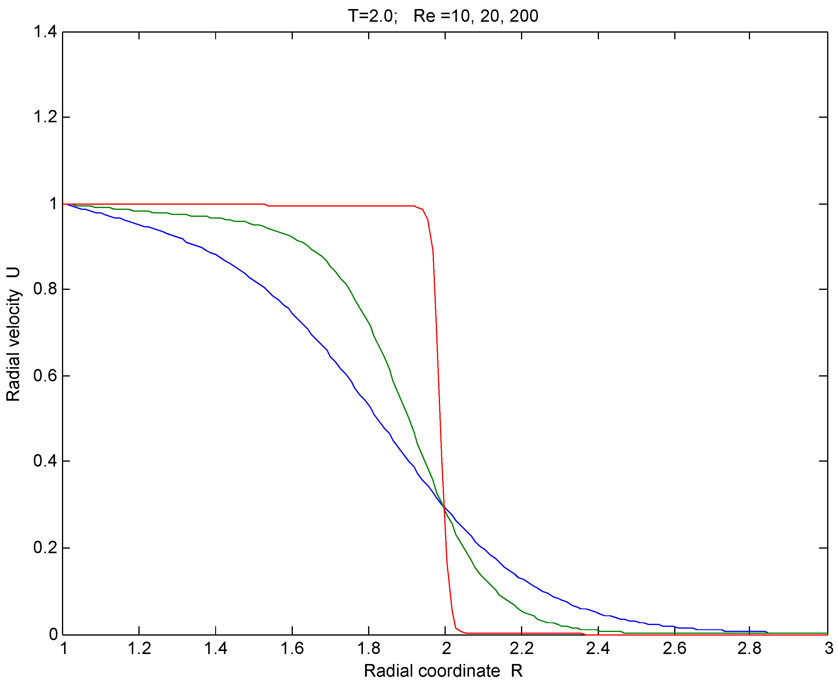
ν is taken to be small, this solution approaches a sharp shock with constant radial speed. The radial solution, depicted in
Figure 1, is in dimensionless units after rescaling by length scale
a and time scale
by which the supply surface has radius
, the fluid speed at (
) is
, the asymptotic travelling wave speed is
, in agreement with the Rankine-Hugoniot relations for a shock, and the Reynolds number is
.
This solution, like others that have been produced, is not consistent with the physics of gas dynamics [
32], in comparison with approximate analytical solutions of the full physical gas dynamics system when pressure, density and entropy are properly taken into account [
30]. However, the exact radial Burgers solution does have some appealing features, such as a realistic inertial term in the momentum equation, and its approach to a viscous shock, that make this exact solution a useful bench test for computational fluids software packages.
Figure 1.
Solution to radial Burgers equation with constant mass supply.
Figure 1.
Solution to radial Burgers equation with constant mass supply.
4. Application of Cole–Hopf to the Schrödinger Equation
The single-particle Schrödinger wave function obeys a linear evolution equation that is analogous to Equation (
4) except that it is necessarily complex valued and wave-like after the viscosity coefficient is replaced by a pure imaginary number:
For convenience, Equation (
20) has been rescaled so that the quantum of action is 1 and the mass is 1. Then the real non-negative particle density satisfies the Liouville conservation equation
where
and the particle current density is
Now the Cole–Hopf transformation is simply
which results in the complex valued vector transport equation
Note that the force per unit mass correctly emerges as
. From the real valued particle density and real valued current density, one may construct a real valued fluid velocity
Note that
is the quantum mechanical phase, whereas
Then the imaginary part of
is
The velocity components
do not satisfy a closed system of transport equations. Instead, they are coupled to the components
:
When the supplementary conditions and are appended, this is a coupled system of nonlinear transport equations. Presumably, similar integrable multi-component systems could be constructed not only from a complex potential but from a quaternion potential or an octonian potential.
The Cole–Hopf transformation links the vector fields
and
as real and imaginary components of a gradient vector
. Without further modifications to the model,
is uniquely determined by
ρ, as in Equation (
24) so that
ρ and
form a closed system. That system is Madelung’s original hydrodynamic analogue [
33] that followed soon after Schrödinger’s publication of the complex wave equation. It has been pointed out [
34] that although the quantum vector field
is not independent, there is a use of it in classical fluid mechanics to refocus on the volume-weighted velocity rather than the mass-weighted velocity [
35]. The two velocity fields
and
that are linked by the Cole–Hopf transformation, are also linked in the measurement of physical quantities. Using the Dirac formalism [
36], the expectation of the energy of a particle in a conservative force field, in a pure state
is
where
in the Schrödinger representation. This can be shown to be equal to
Hence,
is the quantum mechanical correction to the classical kinetic energy density of the Madelung fluid. It may be interesting to extend the irrotational vector fields
and
to be independent fields by adding independent solenoidal contributions:
After breaking the condition , the system of equations for would no longer be equivalent to a linear equation for Ψ but to a system of nonlinear equations for Ψ and . The nonlinear interactions would become negligible asymptotically if there were shear viscosity to dissipate the vorticity, so that could be neglected after some time.
5. Some Relevant Questions in Symmetry Analysis
It is well known (e.g., [
37]) that after neglecting linear superpositions, the generators of Lie point symmetries of a
linear PDE for
take the restricted infinitesimal form
which has an equivalent vertical Lie contact symmetry (e.g., [
37]), in infinitesimal form
The Lie point symmetry classification of the Schrödinger equation with a general potential energy function in two and three dimensions, was completed by Boyer [
38]. After applying such an invariance transformation, the gradient of
is still an irrotational vector that satisfies the complex valued vector transport Equation (
23). Conversely, if a point transformation leaves the system of complex vector transport equation plus condition of irrationality invariant, then the new solution
may be integrated to construct a potential
that is unique up to an additive complex function of
t, equivalent to multiplying Ψ by an arbitrary spatially uniform gauge function
that has no effect on calculating physical expectation values (e.g., [
36]).
From the class of nonlinear scalar parabolic equations, integrability of the one-dimensional Burgers equation hierarchy can be detected by an extended higher-order Lie symmetry analysis (e.g., [
2]) or by a potential Lie symmetry analysis associated with local conservation laws (e.g., [
6]). The system (2) and (3) of six partial differential equations for three functions
of four independent variables
and
t, is integrable. That fact was found by extending the Cole–Hopf transformation that was known from the one-dimensional version. It was not found from symmetry analysis. Using the Cole–Hopf transformation, one may reconstruct Lie–Bäcklund symmetries of the integrable vector system from those of the associated linear scalar equation. From the transformed solution
of the scalar equation, the gradient operation
, preserves the irrotational condition of the vector system. It also must preserve the governing transport equation of the vector transport equation for
. For example, the linear heat equation
is invariant under differentiation in any fixed direction. An elementary third-order Lie–Bäcklund symmetry is
with
the fixed components of a totally symmetric tensor. Then by the substitution
, the corresponding transformation for
is
In the one-dimensional case, all indices are 1 and this reduces to a known Lie–Bäcklund symmetry of the standard Burgers equation (e.g., [
7]):
In the case of the complex Burgers fluid representation of quantum particle dynamics, incorporation of a solenoidal component of the complex fluid velocity
would extend wave mechanics to have not only a scalar wave function, which is a function of the fluid velocity potential, but also a vector potential
that satisfies a system of nonlinear PDE coupled to Ψ. Neither of the two principal founders of wave mechanics, de Broglie and Schrödinger, accepted the Copenhagen interpretation of the probability of outcomes of measurement [
39,
40]. Perhaps they would have found a supplementary classical vector potential more palatable. Since the linear Schrödinger equation correctly describes an evolving particle except when the wave function collapses to a single eigenstate during the decoherence effect of observation by filtering, it can only possibly be the act of measurement that introduces vorticity to the quantum fluid. The coupled nonlinear interaction between
and Ψ may have a complicated ergodic dynamics. The probability density of an energy eigenstate may be the measure of a region in state space that becomes the basin of attraction for a particular eigenstate when the filtering observation is carried out. After the imposed vorticity decays, the state will again evolve according to the Schrödinger equation.
Symmetry classification of some Burgers type systems is carried out in [
41] (higher-order symmetries) and [
42] (Lie and conditional symmetries).
A point symmetry classification of the potential system, with side constraints other than the irrotational condition, looks to be within the capability of symbolic packages, perhaps after making some reasonable ansätze on the functions and . However the complexity of the calculation grows rapidly with the number of variables, for example when one proceeds to tensor transport equations.
In one space dimension, there are other integrable nonlinear diffusion equations that are obtainable from a linear equation for the potential variable, by a change of variable. Under the group of contact transformations, the equivalence classes of these integrable equations are represented by canonical forms [
7] that include the linear equations, the Burgers class,
For example, if
, then the linear equation
is sufficient for Equation (
34). In one dimension, the hodograph transformation is crucial [
43] but in three dimensions it has no simple analogue.
6. Conclusions
From any exact solution of the linearly forced linear heat equation in
n spatial dimensions, one may construct an exact compressible solution to the prototype vector transport equation via a generalisation Equation (
14) of the potential Burgers equation to higher dimensions. The linearisation procedure applies in three dimensions to compressible irrotational flows but not to rotational incompressible flows. For example, there is a simple integrable radial Burgers equation, for which the radial Cole–Hopf potential
obeys the radial heat diffusion equation. In three dimensions,
must satisfy the classical one-dimensional diffusion equation (Chapter 9 of [
31]). This fact has been used to construct an exact radial viscous gas flow with a shock. The simple examples provided above have zero forcing term. However, exact solutions may be constructed similarly for simple conservative force fields such as uniform gravity. Conceivably, hydrodynamic statistical distributions could be calculated from the randomly forced 3D vector transport equation just as for the one-dimensional Burgers equation [
44]. Just like the one-dimensional Burgers equation, this has limited relevance for the interesting physical phenomena of fluid mechanics that involve evolution of vorticity.
By way of contrast, in wave mechanics it is a linear second-order evolution equation, the Schrödinger equation, that is physically relevant. Just as for the case of the linear heat equation, one may apply the reverse Cole–Hopf transformation to the Schrödinger equation, leading to a complex Burgers-type equation that is physically relevant. This is an integrable system of nonlinear transport equations for two real velocity-like vectors. Both the real and imaginary parts of the Burgers velocity have direct physical interpretations, while the squared modulus of the complex velocity is the quantum mechanical correction to kinetic energy density. However, the Cole–Hopf transformation suggests that the integrable gradient flows that are well understood, be extended by adding a rotational component to the velocity-like fields, then carrying out a symmetry classification of the equivalent systems of PDE for the potentials, with additional side conditions other than that of zero vorticity.


