Fluctuating Asymmetry of Plant Leaves: Batch Processing with LAMINA and Continuous Symmetry Measures


Abstract
: Unlike landmark methods for estimating object asymmetry, continuous symmetry measures (CSM) can be used to measure the symmetry distance (ds) of inconsistent objects, such as plant leaves. Inconsistent objects have no homologous landmarks, no consistent topology, no quantitative consistency, and sometimes no matching points. When CSM is used in conjugation with LAMINA Leaf Shape Determination software, one can quickly and efficiently process a large number of scanned leaves. LAMINA automatically generates equally-spaced points around the perimeter of each leaf and the resulting x-y coordinates are normalized to average centroid size prior to estimating ds using a fold, average, unfold algorithm. We estimated shape asymmetry of leaves of three species of flowering plants: Ligustrum sinense (Chinese Privet), Rubus cuneifolius (blackberry), and Perilla frutescens (Perilla), as well as individual leaves from a few species of oaks (Quercus) and maples (Acer). We found that 100 to 200 equally-spaced points worked well for all three of the main species. Measurement error accounted for a small proportion of the asymmetry variation. Nevertheless, measurement error was great enough to generate some negative size scaling after normalization to average centroid size.1. Introduction
Most plant leaves are inconsistent objects having no homologous landmarks, no consistent topology, no quantitative consistency, and few matching points [1]. Consequently, they pose numerous difficulties for biologists studying the fluctuating asymmetry (i.e., random deviations from perfect symmetry) of plants. The usual approach is to measure asymmetry of leaf width or vein length on right and left sides [2,3]. However, these approaches only reflect linear dimensions and it is tedious to process one leaf at a time. Moreover, they do not capture leaf shape. In this paper, we describe a high-throughput approach that can automatically measure the shape asymmetry of ten or more leaves in three steps. This approach requires only a flatbed scanner, LAMINA (Umeå University, Umeå, Sweden) software, and a MATLAB (The MathWorks, Inc., Natick, MA, USA) function that estimates the asymmetry of an object having mirror symmetry.
Continuous symmetry measures can be used to estimate the symmetry distance ds (i.e., asymmetry) of inconsistent objects having variable numbers of structural elements, such as different numbers of lobes, sinuses, and veins on right and left sides of a leaf. These measures were developed for the computer vision and computer graphics community [4,5], and they treat symmetry as a continuous feature [6]. Because continuous symmetry measures quantify asymmetry in all dimensions and for all types of symmetry, they are a flexible tool for analyzing deviations from perfect symmetry in plant leaves. Milner et al. [7,8] and Frid [9], for example, have previously used continuous symmetry measures with anchor points (in contrast to landmarks or semi-landmarks) on left and right sides of leaves. In addition, Frey et al. [10] used continuous symmetry measures to estimate deviations from perfect rotational symmetry of Geranium flowers having five-way rotational symmetry. This was done with petal lengths and angles. Our approach differs in that it relies on several semi-landmarks and one or two true landmarks rather than anchor points or lengths and angles.
Continuous symmetry measures are based on the concept of symmetry groups, which are abstract groups of symmetry-preserving operations (or transforms) [11]. The set of these symmetry-preserving transformations (e.g., reflection, translation, rotation, or a mixture of all three operations) constitute a symmetry group. From the perspective of abstract algebra, a symmetric object is a set of points invariant under the actions of any element of a particular symmetry group. For example, an isosceles triangle in two-dimensions has mirror symmetry (or reflection) and identity (no transformation or rotation through 360°) [6]. An isosceles triangle has one axis of mirror symmetry, which goes through the vertex and the midpoint of the base.
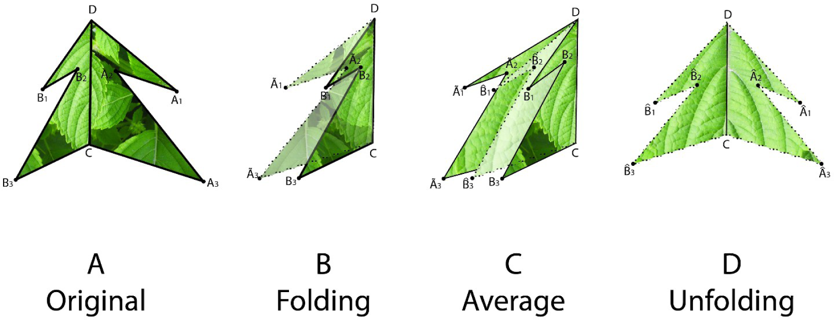
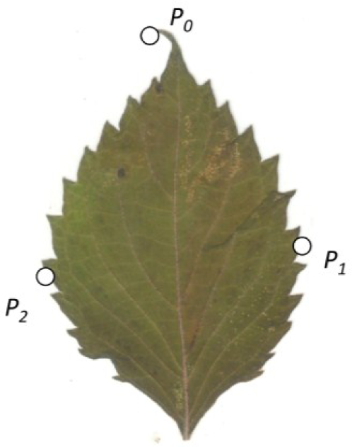
To estimate the symmetry distance ds of an object we first represent it by a sequence of points Pi, i = 1, …, n. We further assume a matching between pairs of these points. The pairing of points is determined by following the points around the object boundary. Since it is assumed that point P0 is at the apex and that the symmetry axis passes through P0, we have that point P0 is paired with itself and point P1 is paired with Pn, P2 with Pn−1 and so on. We then take every pair of matching points (Pj, Pk) and reflect one of the pair across the axes of mirror symmetry (fold), obtaining . Then we average these folded points and obtain a single averaged point for each pair, and reflect these averaged points back across the axes of mirror symmetry (unfold), obtaining (Figure 1). The measure of symmetry distance for the given mirror axis is then , where is the original location of a point and is the location of the point after folding, averaging, and unfolding, and ∥P−Q∥ designates the Euclidean distance between a pair of points P and Q. The set of points is proven to be mirror symmetric and “closest” to the set of points Pi in terms of the Euclidean distance between points (see [6]). If the mirror axis is not given, then the final step is to minimize ds over all possible axes of mirror symmetry. A closed-form solution for finding this optimal mirror axis can be found in [6].
One can interpret the symmetry distance ds as the amount of “effort” required to transform a given shape into a symmetric one. This “effort” is the mean of the squared distances each point must move from its original position to one of perfect symmetry. This approach assumes no a priori symmetric shape to be compared with or transformed into, and it can be generalized to any object in any dimension.
In practice, we evaluate CSM of a leaf by equally spacing points around the margin of the leaf. We further assume a single axis of symmetry, passing through the apex (the first sampled point) and following the midrib. This implies that for the CSM evaluation of ds described above, the mirror symmetry axis is given and the pairing of points is well defined and determined by the order of sampled points around the boundary. With continuous symmetry measures, we can estimate the symmetry distance of leaves for any number of sample points. In practice, we evaluate the symmetry of leaves for various number of sample points between 3 and 200.
2. Methods
We randomly sampled 9 or 10 leaves (or terminal leaflets) from each of 10 individual plants of three species of flowering plants, Ligustrum sinense (Chinese Privet, Oleaceae), Rubus cuneifolius (blackberry, Rosaceae), and Perilla frutescens (Perilla, Lamiaceae). The leaves of these three species differ in size, margin (entire to finely serrate to coarsely serrate), shape (ovate to rhomboid), and flatness of the lamina (flat to wavy or curly). In addition to these leaves, we examined a small number of diverse oak (Quercus velutina, Q. rubra, Q. palustris, Q. alba) and maple (Acer rubrum, A. saccharum) leaves.
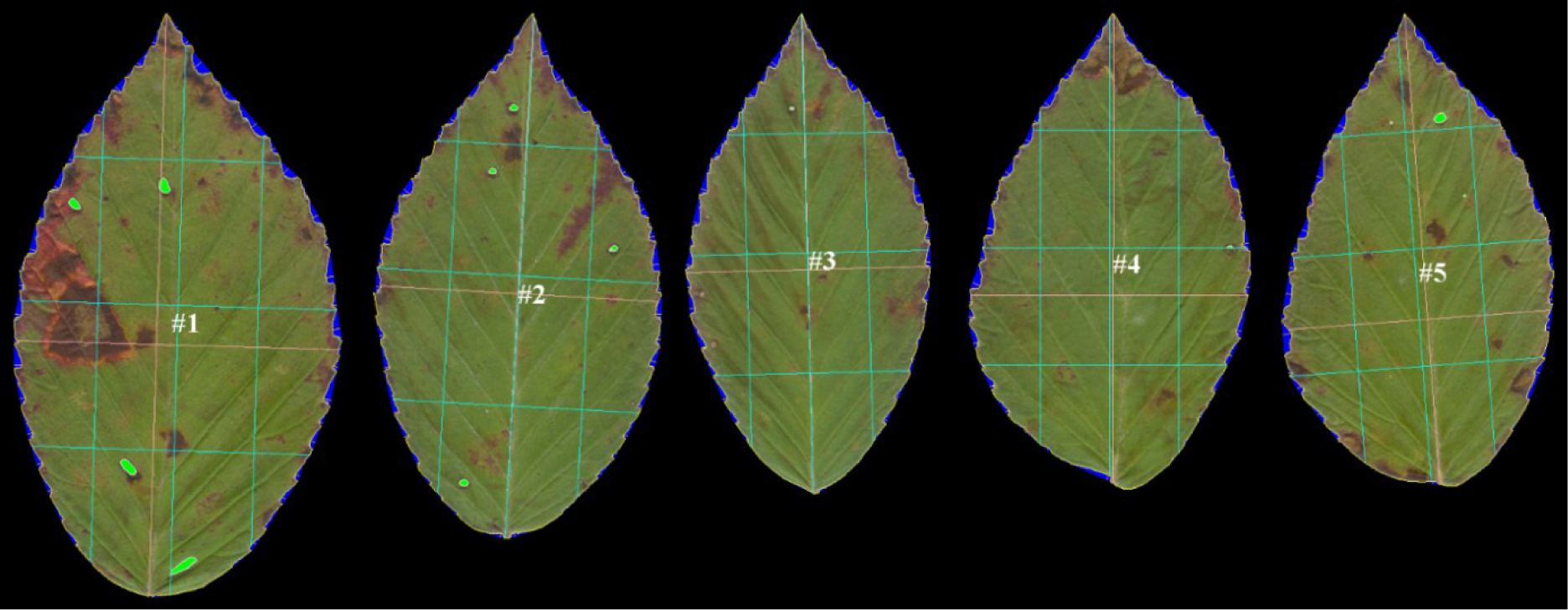
Leaves were pressed for at least 48 hours. The petioles of the leaves were removed, leaving just the lamina and the veins within the lamina. Up to 10 leaves at a time were scanned (HP Scanjet 3500c Series) into a tiff file (300 or 600 dpi, depending on leaf size). Any leaves having herbivore damage to their margins were omitted. The leaves were arranged on the scanner such that the apices of all the leaves were oriented in the same direction and pointing towards the top of the image (Figure 2). These were batch processed using LAMINA software [12].
LAMINA is Leaf Shape Determination software [12]. It can handle batch processing, which makes it particularly worthwhile. It automatically measures surface area, shape, perimeter, leaf serration, herbivory damage (missing leaf area), and several other useful variables, including leaf symmetry. LAMINA’s index of leaf symmetry is the ratio of the linear distance of two lines parallel to the main proximo-distal axis of the leaf (Figure 2); the first vertical green line on the left is the proximo-distal lamina length at 25% of the centro-lateral axis (L) and the third (parallel) green line is the proximo-distal lamina length at 75% of the centro-lateral axis (R). The individual leaf asymmetry is L/R. A ratio of 1 implies a perfectly symmetrical leaf. Taking the log of L/R is equivalent to log L − log R, the most widely used index of signed leaf asymmetry, but instead of leaf widths (perpendicular to the proximo-distal axis) these distances are parallel to it. While certainly useful, these are linear distances and they do not reflect shape asymmetry alone [13]. (For those wishing to use this measure of leaf asymmetry, we note that right-left and top-bottom asymmetry variables are reversed in LAMINA’s output. The output variable labeled Vertical size 25%/Vertical size 75% is the left-right asymmetry, contrary to LAMINA’s own definitions of vertical and horizontal size at 25% and 75% of the respective orthogonal axes.) In addition to all of these variables, one can automatically place a series of equidistant semi-landmarks around the periphery of each leaf (Figure 3). This captures the shape of a leaf.
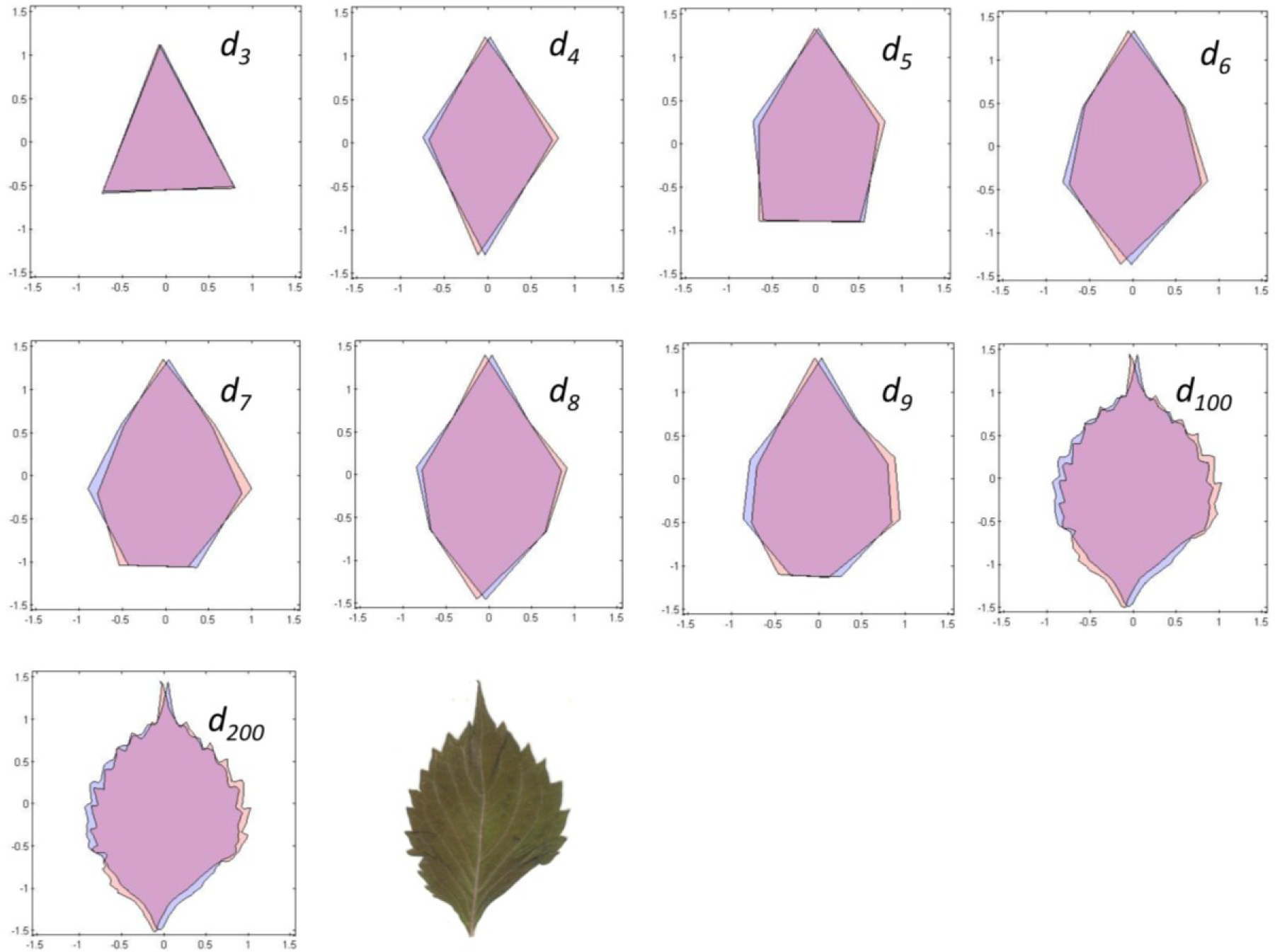
To estimate shape asymmetry, we used LAMINA to automatically place n equidistant points around the perimeter of each leaf, generating the x,y-coordinates of an n-sided object. When n = 3, the object approximates a triangle. Likewise, n = 4 generates a quadrilateral, n = 5 generates a pentagon, n = 6 generates a hexagon, n = 7 generates a heptagon, n = 8 generates an octagon, n = 9 generates a nonagon, and n = 100 and n = 200 generate higher-order objects. The first point is automatically placed at the leaf apex, one of the few consistent landmarks on most leaves.
Before estimating the continuous symmetry measure that reflects shape alone, we computed the centroid (center of mass) of each object and translated the entire object to a centroid of (0,0). We then scaled the centered object so that the average distance between the points to the origin is 1. This step removes the effect of positive size scaling, so that the coordinates capture the shape only. Early tests of the software showed that positive size scaling of leaf asymmetry was the rule for all species of plants we examined, unless we scaled the objects to average centroid size. In fact, positive size scaling was a characteristic of any object scaled up or down by a constant factor. LAMINA also seems to reverse the polarity of the y-axis, and while this does not influence the estimates of asymmetry, we flipped the y-axis by multiplying all ys by −1. This makes it easier to interpret the graphical output if we need to superimpose objects.
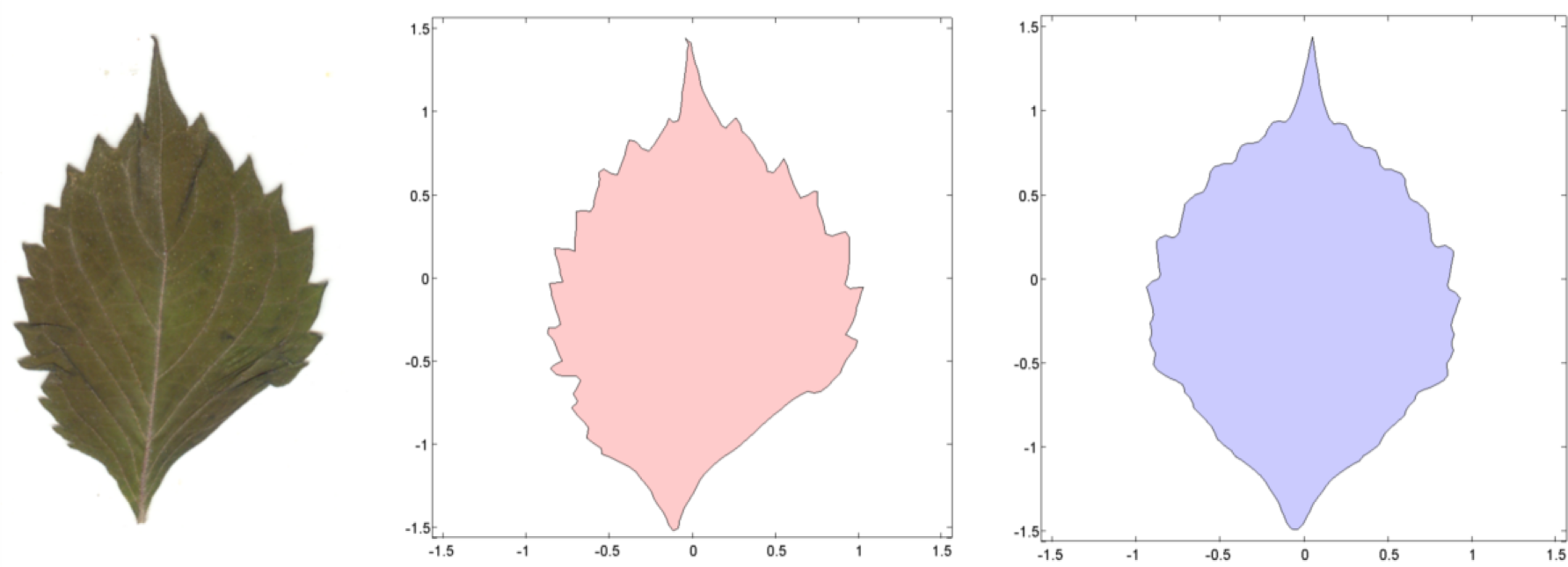
To estimate a continuous symmetry measure (CSM) for an object having mirror symmetry, we used code written in MATLAB [14]. The code computes a symmetry distance ds for a two-dimensional object having mirror symmetry. It returns the value of ds, the new x,y-coordinates of the symmetrized object, and θ (the angle in radians between the reflection angle and the y-axis). This program takes the x,y-coordinates and deforms them into a perfectly symmetrical object having mirror symmetry (Figures 4 and 5).
The continuous symmetry measure on an n-sided object is defined as:
To estimate ds as efficiently as possible, we combined all of the LAMINA output into an Excel data file. Then we created a subfile from the last 2n columns of the data file; these contain the x,y-coordinates of the n points of the object. In MATLAB, we used xlsread to read the Excel subfile of x- and y-coordinates. We then used two scripts (GenericRows and genericApplyToRows) to apply the functions NormalizePoints.m and csm_Mirror_closedBoundary.m to every row in the vector of x,y-coordinates. NormalizePoints.m translates the object to a centroid of (0,0) and scales it to average centroid size. The function csm_Mirror_closedBoundary.m first converts each row (a 1 × 2n vector) into a 2 × n matrix and then calculates cval (ds), ncoor (new coordinates), and theta (θ, the angle that the axis of symmetry makes with the y-axis). We used xlswrite to convert the MATLAB output back into Excel, and combined it all with the original data file for statistical analysis in SPSS.
With continuous symmetry measures of any object, there is always the possibility of a less than optimal solution. Such a non-optimal solution would have an axis of symmetry other than the leaf’s main axis of mirror symmetry, which ordinarily runs along its midrib and through P0. For n = 3, for example, it is possible that the closest object having mirror symmetry may be through one of the other two vertices (P1, P2). But because we constrained the axis of mirror symmetry to pass vertically through the leaf apex, P0, it is likely that the axis will parallel the leaf’s midrib. To check for this, we plotted the original coordinates against the new symmetrized coordinates (Figures 4 and 5). Any instability should be immediately obvious from a visual inspection and should be associated with a large value of θ; if the leaves have been arranged properly on the scanner the reflection angle should be nearly parallel to the y-axis (θ ≈ 0). A value of θ > 0.2–0.3 radians should be examined closely.
Because measurement error can inflate measures of dispersion, and ds measures shape variation (dispersion) between left and right sides of a leaf, one must estimate measurement error of, at least, a subsample of leaves. Consequently, we did five replicate scans of a subset of 10 leaves of each species to estimate measurement error. We estimated variance components in SPSS for leaf asymmetry (d200) among individuals, among leaves within individuals, and among replicate scans. Variation among estimates within a scan were negligible.
Size scaling of asymmetry is a serious concern in all studies of fluctuating asymmetry [1]. Consequently, we used linear regression and correlation to see if ds varied with leaf area.
3. Results
An examination of all of the leaves with values of θ > 0.2 revealed no evidence of non-optimal solutions. These non-optimal solutions would have had axes of symmetry other than the main leaf axis (apex to base of the petiole). When examined closely, all of the leaves that had higher values of θ had been accidentally placed somewhat off the vertical axis. Quickly closing the top of the scanner on a leaf can sometimes shift its position.
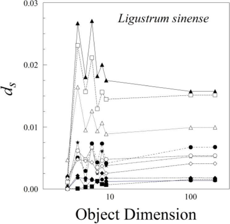
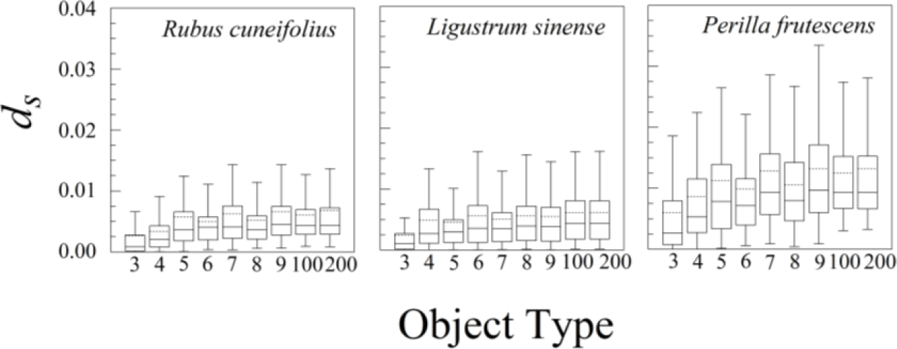
The nine different kinds of objects (n = 3 through n = 200) give roughly similar leaf asymmetries, though the symmetry distances based upon 100 or 200 points usually had the smallest interquartile ranges (Figure 6).
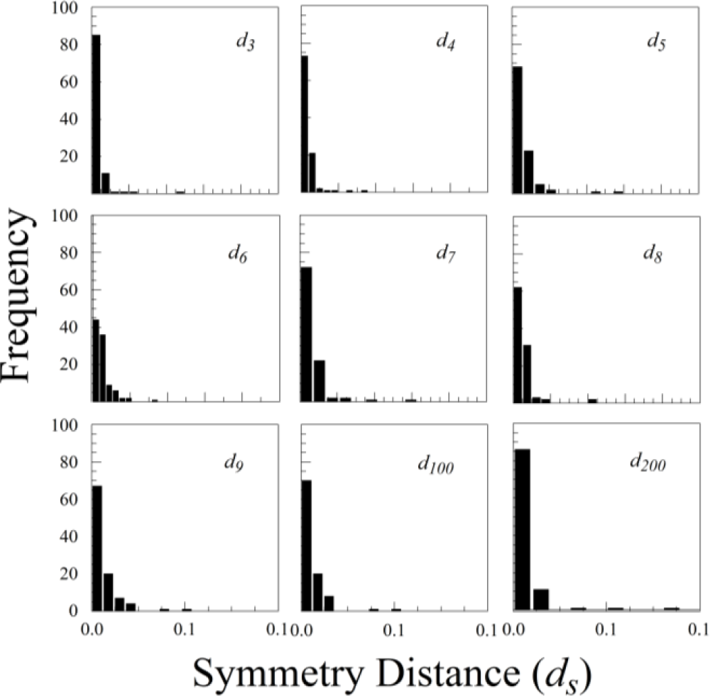
The statistical distributions of ds for all three species were highly skewed, with a mode close to zero (see Figure 7 for Rubus cuneifolius). The distributions are best fit by either an exponential distribution or a half-normal distribution.
The various results of the lower-sided objects are unstable in the sense that, for a pair of leaves (A and B) and asymmetry of A > B for d3, it does not follow that A > B for d4, d5, d6, or dn (Figure 8). The low-sided objects, such as n = 3, seem to be less stable than the higher sided ones. The lines connecting ds for n = 100 and n = 200 are roughly parallel, whereas those for triangles (n = 3) and quadrilaterals (n = 4) often cross. Moreover, odd- and even-sided objects seem to capture somewhat different aspects of leaf shape asymmetry.
Nearly all of the measurement error of ds was due to variation among scans; variation among replicate processing of the same scan was negligible (effectively zero). Measurement error of d200 was fairly consistent among species, ranging from 0.118 × 10⁻⁵ for Rubus cuneifolius to 1.088 × 10⁻⁵ for Ligustrum sinense and 1.179 × 10⁻⁵ for Perilla frutescens. The percentage of measurement error, however, varied greatly among species, mainly because the variation in ds among leaves within an individual was so great. The percentage of measurement error ranged from 1.05% for Perilla frutescens to 5.02% for Rubus cuneifolius and 45.23% for Ligustrum sinense. Because ds is analogous to a variance (it is the average of squared distances rather than squared deviations), we can also compare measurement error on a leaf-by-leaf basis by comparing the mean of ds for a particular leaf with its variance. This measurement error as a percentage of the mean of ds ranged from 0.0165% for Perilla frutescens to 0.0228 for Rubus cuneifolius and 0.1798% for Ligustrum sinense.
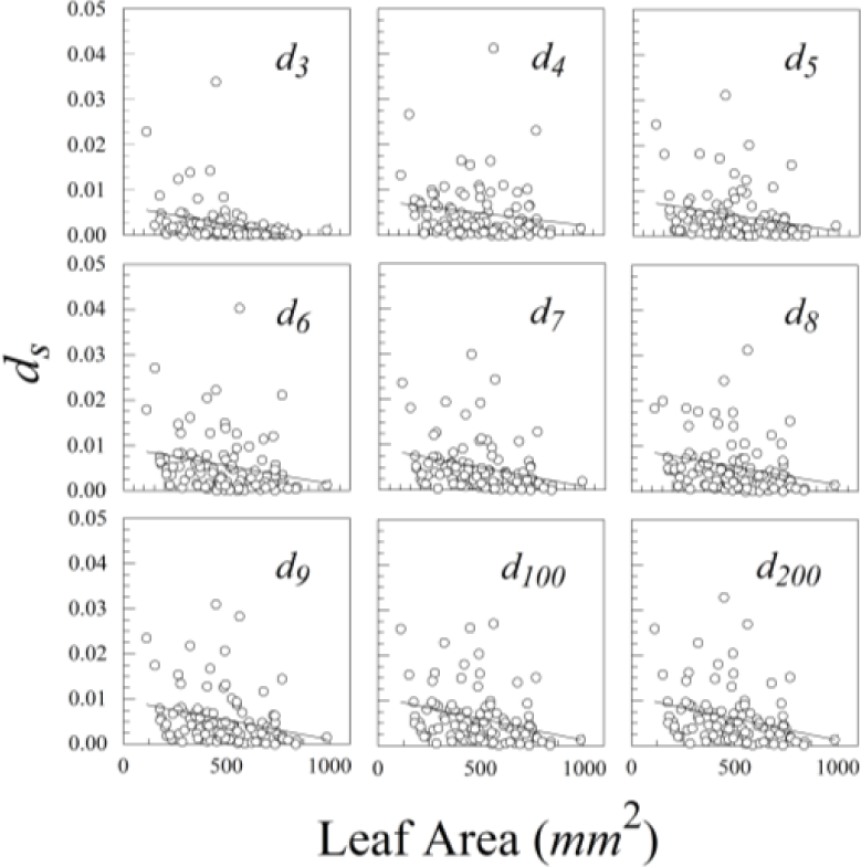
Ligustrum sinense leaves showed significant negative size scaling for ds (Figure 9 and Table 1). Rubus cuneifolius and Perilla frutescens also showed negative size scaling, though it was not statistically significant.
In addition to analyzing leaves of Ligustrum sinense, Rubus cuneifolius, and Perilla frutescens, we also looked at leaves of several oaks and maples. Many of the oak leaves, in particular, were fairly asymmetrical and have large lobes and sinuses. The CSM program handled these well, though the symmetrized versions of the leaves did not always look natural, especially if the original leaf was extremely asymmetrical (Figure 10).
4. Discussion
LAMINA software, in conjunction with continuous symmetry measures, can be used to estimate the shape asymmetry of plant leaves. Our method, which is based on the mirror symmetry of irregular objects, gives usable estimates of ds, the symmetry distance, for objects having from three to at least 200 sides (i.e., triangles to many sided n-gons).
4.1. Shape Asymmetry
The shape of an object, or landmark configuration, is “all of the geometric information remaining … after differences in location, scale, and rotational effects are removed” [13]. Most leaves, however, have just two stable landmarks, which is insufficient to estimate shape. And because these landmarks are on the axis of mirror symmetry, they cannot be used by themselves to estimate shape asymmetry. One of these landmarks is the leaf apex, where the mid-vein intersects the leaf margin at the leaf tip. The other is the point where the petiole connects with the leaf lamina. LAMINA allows us to establish just one of these landmarks, the leaf apex. If both true landmarks are known, they can be used in csm_Mirror_closedBoundary.m [14] to force the axis of mirror symmetry through both points. The other equidistant points, proceeding clockwise around the leaf margin from the apex, are semi-landmarks, defined with respect to the leaf apex [13,15]. Semi-landmarks represent less information than true landmarks, and they consequently have fewer degrees of freedom. Nevertheless, they serve well in estimating shape asymmetry.
To get at the “shape” of a leaf, we scale irregular objects to average centroid size, and translate the centroid to (0,0). We do not rotate the objects about their centroid, because it is irrelevant to our estimates of symmetry distance (ds).
4.2. Cautions and Limitations
Instability of the algorithm should be greatest for leaves approaching a circular shape, such as those of Tropaeolum majus L. When n = 3, the boundary points of a close-to-circular leaf should approach an equilateral rather than an isosceles triangle. An equilateral triangle has three axes of mirror symmetry, whereas an isosceles triangle has just one. The same reasoning can be extended to objects having n = 4, 5, 6, 7, or more points. A quadrilateral, for example, based on the outline of a perfectly ovate leaf could easily have two axes of mirror symmetry (one parallel to the midrib and the other perpendicular to it).
With our algorithm, however, the axis of symmetry is constrained to pass through P0. Consequently, axes of symmetry perpendicular to the midrib are impossible. Nevertheless, if we had not constrained the axis of symmetry in such a way, we could have detected (and avoided) such results by examining the original and the symmetrized objects of the leaves. One can also examine just the leaves having the greatest values of θ. We observed no problems, even with the most asymmetric of leaves. We have noticed that odd- and even-sided objects seem to capture somewhat different aspects of leaf shape asymmetry. According to Savriama and Klingenberg [16], if an object is assimilated as either a symmetric shape with an odd or even order of symmetry, the components of asymmetry will differ.
For even-sided objects, one of the semi-landmarks is invariably close to the base of the petiole. This is not true of odd-sided objects. Even-sided objects also tended to have smaller interquartile ranges. None of this should be a problem, however, if the number of equidistant points is large enough.
A final limitation is the practical number of leaves that can be scanned at once. Even with a very large scanner, we have noticed that LAMINA cannot handle very large image files. Consequently, we either reduced the number of leaves scanned at once, or reduced the resolution (dpi) from 600 or 300 to something smaller.
4.3. Directional Asymmetry and Antisymmetry
Within the context of continuous symmetry measures, shape asymmetry cannot be easily classified into fluctuating asymmetry, directional asymmetry, or antisymmetry. Directional asymmetry exhibits a distribution of L − R whose mean is not zero (i.e., μL − R ≠ 0). The mammalian heart, for example, is directionally asymmetric; the left side is normally larger than the right side [17]. Antisymmetry, on the other hand, describes a bimodal (or platykurtic) distribution of L − R and a mean of zero (μL − R = 0). The value of ds implies no polarity or directionality (ds ≥ 0). Moreover, the concept of shape is more abstract than concepts of distance, length, mass, or number, which can all have direction. Finally, different parts of an object can have asymmetry in different directions.
4.4. Size Scaling
Some negative size scaling remains after rescaling each object to average centroid size. This is likely a consequence of the mixing of additive and multiplicative error [1,18]. Growth variation is multiplicative, whereas measurement error is additive. These are mixed together whenever one measures a leaf. For small leaves, measurement error makes up a greater proportion of the asymmetry variation. When one corrects for multiplicative error by taking the logs of L and R or by scaling an object to average centroid size, one includes additive error in the correction. Small leaves appear more variable and large leaves appear less variable.
The simplest way of dealing with this issue is to average replicate measurements of ds. Each round of averaging replicates reduces measurement error by one half, until it is inconsequential. This requires, however, quite a bit of additional work, rescanning and re-measuring leaves.
Another approach is to use a Box-Cox (power) transformation, , that minimizes the regression of ds on leaf area (or centroid size). Unfortunately, different species of plants may require different transformations, because the proportion of measurement error may vary from species to species. Raz et al. [9], for example, used power transforms to compare leaf asymmetries of several species of plants on north- and south-facing slopes of Evolution Canyon, Israel.
Of our three species of plants, only Ligustrum sinense showed significant negative size scaling. Unsurprisingly, this species also had the highest proportion of measurement error, and consequently the greatest mixing of additive and multiplicative error. The problem of such mixture distributions will have to be solved if one expects to compare leaf asymmetries of different species of plants.
4.5. Future Work
We have just examined irregular objects having a maximum of 200 vertices. But LAMINA can output more semi-landmarks than that. Future work should examine the behavior of leaf-shaped objects having many more vertices. For our three species, estimates of ds seemed to converge for n > 100.
For future work, we plan to examine leaf shape asymmetry in more species than just these three. We are presently exploring leaf asymmetry of paired native and invasive exotic species. We are also looking at shape asymmetry of leaves in highly polluted environments and we are looking at leaf asymmetry of r- and k-selected species (annuals and perennials).
5. Conclusions
We describe a new approach, continuous symmetry measures (CSM), to measuring leaf shape asymmetry. Previous approaches have used anchor points [7–9] and distances and angles of rotationally symmetric flowers [10]. Landmark methods [19] might be suitable for some leaves that have consistent topology, but we are unaware of any such published studies involving true landmarks.
Although three to nine points do not capture leaf shape well, they do capture some aspects of leaf shape asymmetry. The leaf apex P0 is a stable point, one of only two stable landmarks on most leaves. However, any irregularity of the leaf margin on right and left sides will shift the positions of P1 through Pn, thereby increasing the estimate of leaf asymmetry.
Because the variation in the estimate of ds decreases with the number of points (sides), we suggest using 100 or 200 points rather than smaller numbers.
Acknowledgments
We thank Zahra Mohamed and Tom Sheehan for helping in the lab. Two referees made valuable suggestions for improving the manuscript. Catherine Chamberlin-Graham helped with the literature search, photography, and proofread the draft. John H. Graham was supported by an endowed chair from Berry College.
Author Contributions
John H. Graham wrote the paper, did the statistical analyses, and the MATLAB analyses. Mattie J. Whitesell and Mark Fleming II collected the leaves and the leaf data. Hagit Hel-Or wrote the CSM software and wrote the parts of the paper devoted to the software and algorithm. Shmuel Raz and Eviatar Nevo assisted with the writing of the paper and with the figures.
Conflicts of Interest
The authors declare no conflict of interest.
References
- Graham, J.H.; Raz, S.; Hel-Or, H.; Nevo, E. Fluctuating asymmetry: Methods, theory, and applications. Symmetry 2010, 2, 466–540. [Google Scholar]
- Freeman, D.C.; Graham, J.H.; Emlen, J.M. Developmental stability in plants: Symmetries, stress and epigenesis. Genetica 1993, 89, 97–119. [Google Scholar]
- Freeman, D.C.; Graham, J.H.; Emlen, J.M.; Tracy, M.; Hough, R.A.; Alados, C.; Escós, J. Plant developmental instability: New measures, applications, and regulation. In Developmental instability: Causes and consequences; Polak, M., Ed.; Oxford University Press: New York, NY, USA, 2003; pp. 367–386. [Google Scholar]
- Zabrodsky, H.; Peleg, S.; Avnir, D. Continuous symmetry for shapes. In Aspects of visual form processing; Arcelli, C., Cordella, L., Sanniti di Baja, G., Eds.; World Scientific Publishing: Singapore, 1994; pp. 594–613. [Google Scholar]
- Liu, Y.; Hel-Or, H.; Kaplan, C.S.; Van Gool, L. Computational Symmetry in Computer Vision and Computer Graphics; Now Publishers Inc.: Hanover, MA, USA, 2009; p. 195. [Google Scholar]
- Zabrodsky, H.; Peleg, S.; Avnir, D. Symmetry as a continuous feature. Pattern Anal. Mach. Intell. IEEE Trans. 1995, 17, 1154–1166. [Google Scholar]
- Milner, D.; Raz, S.; Hel-Or, H.; Keren, D.; Nevo, E. A new measure of symmetry and its application to classification of bifurcating structures. Pattern Recognit. 2007, 40, 2237–2250. [Google Scholar]
- Milner, D.; Hel-Or, H.; Keren, D.; Raz, S.; Nevo, E. Analyzing symmetry in biological systems. Proceedings of IEEE International Conference on Image Processing, Genova, Italy, 1–14 September 2005; pp. 361–364.
- Frid, A. Merging Local and Global Symmetry. M.S. Thesis, University of Haifa, Haifa, Israel, 2008. [Google Scholar]
- Frey, F.M.; Robertson, A.; Bukoski, M. A method for quantifying rotational symmetry. New Phytol. 2007, 175, 785–791. [Google Scholar]
- Weyl, H. Symmetry; Princeton University Press: Princeton, NJ, USA, 1952. [Google Scholar]
- Bylesjö, M.; Segura, V.; Soolanayakanahally, R.Y.; Rae, A.M.; Trygg, J.; Gustafsson, P.; Jansson, S.; Street, N.R. Lamina: A tool for rapid quantification of leaf size and shape parameters. BMC Plant Biol. 2008, 8. [Google Scholar] [CrossRef]
- Zelditch, M.L.; Swiderski, D.L.; Sheets, H.D. Geometric Morphometrics for Biologists: A Primer; Academic Press: Waltham, MA, USA, 2012. [Google Scholar]
- MATLAB Code for Continuous Symmetry Measures (CSM) of Leaves and Other Objects. Available online: http://facultyweb.berry.edu/jgraham/CSMCode.htm accessed on 10 March 2015.
- Bookstein, F.L. Landmark methods for forms without landmarks: Morphometrics of group differences in outline shape. Med. Image Anal. 1996/7, 1, 225–243. [Google Scholar]
- Savriama, Y.; Klingenberg, C.P. Beyond bilateral symmetry: Geometric morphometric methods for any type of symmetry. BMC Evolut. Biol. 2011, 11. [Google Scholar] [CrossRef]
- Graham, J.H.; Emlen, J.M.; Freeman, D.C.; Leamy, L.J.; Kieser, J.A. Directional asymmetry and the measurement of developmental instability. Biol. J. Linn. Soc. 1998, 64, 1–16. [Google Scholar]
- Graham, J.H.; Shimizu, K.; Emlen, J.M.; Freeman, D.; Merkel, J. Growth models and the expected distribution of fluctuating asymmetry. Biol. J. Linn. Soc. 2003, 80, 57–65. [Google Scholar]
- Klingenberg, C.P.; McIntyre, G.S. Geometric morphometrics of developmental instability: Analyzing patterns of fluctuating asymmetry with procrustes methods. Evolution 1998, 52, 1363–1375. [Google Scholar]


| Species | Object Type
| ||||||||
|---|---|---|---|---|---|---|---|---|---|
| d3 | d4 | d5 | d6 | d7 | d8 | d9 | d100 | d200 | |
| Rubus cuneifolius | −0.027 | −0.158 | 0.007 | −0.126 | −0.046 | −0.115 | −0.068 | −0.110 | 0.196 |
| (0.788) | (0.118) | (0.947) | (0.211) | (0.652) | (0.253) | (0.502) | (0.277) | (0.051) | |
| Ligustrum sinense | −0.313** | −0.165 | −0.233* | −0.227* | −0.277** | −0.251* | −0.265** | −0.294** | −0.285** |
| (0.002) | (0.102) | (0.020) | (0.023) | (0.005) | (0.012) | (0.008) | (0.003) | (0.004) | |
| Perilla frutescens | −0.040 | −0.077 | −0.130 | −0.088 | −0.129 | −0.117 | −0.106 | −0.096 | −0.124 |
| (0.705) | (0.470) | (0.223) | (0.408) | (0.226) | (0.274) | (0.321) | (0.370) | (0.245) | |
© 2015 by the authors; licensee MDPI, Basel, Switzerland This article is an open access article distributed under the terms and conditions of the Creative Commons Attribution license (http://creativecommons.org/licenses/by/4.0/).
Share and Cite
Graham, J.H.; Whitesell, M.J.; II, M.F.; Hel-Or, H.; Nevo, E.; Raz, S. Fluctuating Asymmetry of Plant Leaves: Batch Processing with LAMINA and Continuous Symmetry Measures. Symmetry 2015, 7, 255-268. https://doi.org/10.3390/sym7010255
Graham JH, Whitesell MJ, II MF, Hel-Or H, Nevo E, Raz S. Fluctuating Asymmetry of Plant Leaves: Batch Processing with LAMINA and Continuous Symmetry Measures. Symmetry. 2015; 7(1):255-268. https://doi.org/10.3390/sym7010255
Chicago/Turabian StyleGraham, John H., Mattie J. Whitesell, Mark Fleming II, Hagit Hel-Or, Eviatar Nevo, and Shmuel Raz. 2015. "Fluctuating Asymmetry of Plant Leaves: Batch Processing with LAMINA and Continuous Symmetry Measures" Symmetry 7, no. 1: 255-268. https://doi.org/10.3390/sym7010255
APA StyleGraham, J. H., Whitesell, M. J., II, M. F., Hel-Or, H., Nevo, E., & Raz, S. (2015). Fluctuating Asymmetry of Plant Leaves: Batch Processing with LAMINA and Continuous Symmetry Measures. Symmetry, 7(1), 255-268. https://doi.org/10.3390/sym7010255