Abstract
In this paper, we develop a general framework for studying Dirichlet Boundary Value Problems (BVP) for second order symmetric implicit differential systems satisfying the Hartman-Nagumo conditions, as well as a certain non-expandability condition. The main result, obtained by means of the equivariant degree theory, establishes the existence of multiple solutions together with a complete description of their symmetric properties. The abstract result is supported by a concrete example of an implicit system respecting -symmetries.
Keywords:
symmetric BVP; second order implicit Ordinary Differential Equation (ODE); multiple solutions; a priori bounds; equivariant degree; multivalued maps; dihedral group symmetries AMS Subject Classification:
Primary: 37C80, 34B16, 47H11; Secondary: 34A26, 37C25, 47H09
1. Introduction
1.1. Subject and Goal
Boundary value/periodic problems for second order nonlinear Ordinary Differential Equations (ODEs) have been within the focus of the nonlinear analysis community for a long time (see, for example [1,2,3]). In [2,4], P. Hartman established the existence result for the boundary value problem:
where the function, , satisfies the so-called Hartman-Nagumo conditions, which, informally, means that f is a reasonable function having a sub-quadratic growth on . Later on, H.W. Knobloch [5,6] observed that a similar result is true for the corresponding periodic problem:
Several extensions of Hartman-Knobloch results of perturbations of the ordinary vector p-Laplacian operator were suggested by J. Mawhin et al. (see, for example, [7,8,9] and the references therein).
Although Hartman’s existence result was extended to more general settings by many authors, to the best of our knowledge, the problems of estimating a minimal number of solutions to (1), as well as classifying their symmetric properties have not been carefully studied. To some extent, our recent paper [10] opened a door to a systematic usage of the equivariant degree theory for analysis of multiple solutions to symmetric (1) and its generalizations. The starting point for our discussion was Example 6.1 from [11] in which a particular case of BVP (1) in the presence of -symmetries was considered (see also [12] in which a “multivalued perturbation of this example” was discussed).
The goal of this paper is to study multiple solutions to boundary value problems for implicit symmetric second order differential systems using the equivariant degree-based method. To simplify our exposition, we will restrict ourselves to the Dirichlet boundary conditions. More specifically, we are interested in the BVPs of the form:
where is an orthogonal G-representation and is a G-equivariant map satisfying the so-called Carathéodory condition. For some motivating examples from mechanics (including, in particular, the ones modeled by the so-called generalized Liénard equation), we refer the reader to [13] and the references therein.
1.2. Method
The main idea behind the method allowing us to study (3) can be traced back to [14,15]. Namely, assume that h satisfies the Hartman-Nagumo conditions with respect to , and, in addition, it is non-expansive with respect to . Since the set of fixed points of a non-expansive map of an Euclidean space is convex, one can canonically associate with problem (3) the “explicit” differential inclusion of the form:
with (here, stands for the set of all non-empty convex and compact subsets of V). By the (equivariant) homotopy argument, the later problem can be reduced to the “explicit” single-valued symmetric BVP of the form of Equation (1), and the equivariant degree-based method developed in [10] can be applied.
Recall that the equivariant degree is a topological tool allowing “counting” orbits of solutions to (symmetric) equations in the same way as the usual Brouwer degree does, but according to their symmetric properties. This method is an alternative and/or complement to the equivariant singularity theory developed by M. Golubitsky et al. (see, for example, [16]), as well as to a variety of methods rooted in Morse Theory, Lusternik-Schnirelmann Theory and Morse-Floer complex techniques (see, for example, [17,18,19,20]) used for the treatment of variational problems with symmetries. These standard methods, although being quite effective in the settings in which they are usually applied, encounter technical difficulties when: (i) the group of symmetries is large; (ii) multiplicities of eigenvalues of linearizations are large; (iii) phase spaces are of a high dimension; and (iv) the operators involved exhibit a lack of smoothness. Furthermore, one would expect to use computer routines for complex computations, while it is not clear if these approaches are “open enough” to be computerized. On the other hand, the equivariant degree theory has all the attributes allowing its application in settings related to (i)–(iv), and in many cases, it allows computerization. For instance, in the case of the dihedral group, the tools required for the symbolic computations of the equivariant degree can be found at [21]. For a detailed exposition of the equivariant degree theory, we refer the reader to [11,22,23,24,25].
1.3. Overview
After the Introduction, the paper is organized as follows. In Section 2, we collect the standard equivariant background together with basic properties of the equivariant degree (without free parameters) for compact equivariant multivalued fields. This theory is applied in Section 3 for studying “explicit” second order equivariant inclusions (see (11)). We reformulate (11) as a fixed-point problem with a compact equivariant multivalued vector field defined on the Sobolev space, , and associate to this field an invariant, , expressed in terms of the equivariant degree (see (22)). Using , we formulate our result for (11) (see Theorem 3.6). In Section 4, we combine Theorem 3.6 with the equivariant version of the well-known result from [15] (cf. Lemma 4.1) to obtain our main abstract result for the “explicit” BVP (3) (in fact, this result (see Theorem 4.4) is expressed in terms of provided by Lemma 4.1). In Section 5, we describe a wide class of BVPs (3) symmetric with respect to the dihedral group representations for which Theorem 4.4 can be applied to obtain a complete symmetric classification of solutions (see Proposition 5.1). We also give a concrete -symmetric example supporting Proposition 5.1 (see Theorem 5.2). To make our exposition self-contained, we conclude with two Appendices (Appendix 1 is related to the equivariant degree theory for single-valued maps (in particular, the concept of a Burnside ring, and a computational formula for the equivariant degree of a linear equivariant isomorphism is given); in Appendix 2, we collected all the facts frequently used in this paper that are related to -representations and -equivariant degree).
2. G-Actions and Equivariant Degree without Parameters for Multivalued Fields
In this section, we briefly recall the standard “equivariant jargon” and present basic facts related to the equivariant degree without free parameters for equivariant multivalued fields. In what follows, G stands for a finite group and V for an orthogonal G-representation.
2.1. G-Actions
For a subgroup, , denote by the normalizer of H in G, by , the Weyl group of H in G, and by , the conjugacy class of H in G. The set, , of all conjugacy classes in G admits a partial order defined as follows: if and only if for some .
For a G-space, X and , denote by the isotropy of x and by the orbit of x. Given an isotropy, , call the orbit type in X and put . Furthermore, for a subgroup, , put . As is well known (see, for instance, [26]), the G-action on X induces a natural -action on .
Consider two subgroups, , of G and put . Clearly, is an -space. Define the number having very transparent geometric meaning; it is equal to the cardinality of the set .
Let X and Y be two G-spaces. A continuous map, , is said to be G-equivariant (or, simply, a G-map) if for all and .
Convention: For a (finite) group, G, we denote by , , , ..., the complete list of all irreducible orthogonal (real) G-representations.
Suppose that V is an orthogonal G-representation (in general, reducible). Then, it is possible to represent V as the following direct sum:
called the G-isotypical decomposition of V, where the isotypical components are modeled on the irreducible G-representations, . In other words, the component, , is the minimal subrepresentation of V containing all the irreducible subrepresentations of V that are equivalent to . Notice that if is a G-equivariant linear operator, then for all k. Furthermore, denote by the set of all linear G-equivariant isomorphisms, .
Let be a Banach space of reasonable (e.g., continuous, differentiable, Sobolev differentiable, etc.) functions, , where V is an orthogonal G-representation. Then, can be equipped with the structure of a Banach G-representation by letting:
Combining Equations (5) and (6) yields the isotypical decomposition:
2.2. Equivariant Degree for Multivalued Vector Fields
In order to treat implicit symmetric BVPs, we will use an extension of the equivariant degree without free parameters to multivalued compact equivariant vector fields with compact convex images. Up to several standard steps, such an extension is very simple (see, for example, [12]). Therefore, below, we will only outline the key steps of the construction (we refer the reader to Appendix 1 of the present paper, where the axiomatic definition for single-valued fields is presented).
Let be a Banach space. Denote by (respectively ) the family of all non-empty convex subsets of (respectively all non-empty convex and compact subsets of ). Let X be a subset of a Banach space, . A map, (respectively ), is called a multivalued map with convex values from X to (respectively multivalued map with convex and compact values from X to ).
A multivalued map, , is said to be upper semi-continuous (in short, u.s.c.) if for every open set, , the set, , is open in X. A u.s.c multivalued map, , is called compact if, for any bounded set, , the closure of is compact in . In what follows, we will write to indicate that F is a u.s.c. compact multivalued map with non-empty compact convex values.
Assume now that and are isometric Banach G-representations, is a G-invariant set and is a multivalued map from X to . Then, F is called G-equivariant if for all and , and we write . Observe that if is a single-valued compact G-equivariant map, then it can also be considered as the multivalued map , . Clearly, is u.s.c. (as a multivalued map) and, therefore, .
Let be an open bounded G-invariant subset. Similarly to the single-valued case, a multivalued map, , is called an Ω-admissible compact G-equivariant field if the following two conditions are satisfied:
- (i)
- there exists , such that and for all ;
- (ii)
- for all , , i.e., (by the same token, F has no fixed-points in ).
In such a case, is called an admissible G-pair in . Denote by the set of all such admissible G-pairs in and put:
(here, the union is taken over all isometric Banach G-representations).
Take . Then, are said to be equivariantly Ω-admissibly homotopic if there exists a multivalued map, , , such that:
- (a)
- , , for all ;
- (b)
- for all .
Lemma 2.1.
(cf. [12,27]).
(i) For any , there exists an equivariant Ω-admissible homotopy, , , such that and , where is a single-valued field.
(ii) Let , be an equivariant Ω-admissible homotopy, such that and , where are (compact) single-valued fields. Then, there exists a single-valued equivariant Ω-admissible homotopy joining and .
Lemma 2.1 allows us to extend the G-equivariant degree defined for single-valued admissible G-pairs to the fields from . Namely, take . Find an admissible G-pair with single-valued , such that is equivariantly Ω-admissibly homotopic to (cf. Lemma 2.1(i)), and put:
Using Lemma 2.1(ii), one can easily verify that , defined by (9), is independent of a choice of a single-valued representative, f. Moreover, by applying the standard argument, one can show that satisfies the standard properties. More precisely:
Theorem 2.2.
where the multiplication “·” is taken in the Burnside ring, (see Appendix 1, Subsection A1.1.).(cf. [12]).
There exists a unique map, , which assigns to every admissible G-pair an element, , called the G-equivariant degree (or, simply, G-degree) of on Ω:
satisfying (among others) the following properties:
- (M1)
- (M2)
- (Additivity) Let and be two disjoint open G-invariant subsets of Ω, such that, for any , one has . Then:
- (M3)
- (Homotopy) If is an Ω-admissible G-homotopy of multivalued G-equivariant compact fields, then:
- (M4)
- (Normalization) Let Ω be a G-invariant open bounded neighborhood of zero in . Then:
- (M5)
- (Multiplicativity) For any
For the equivariant topology/representation theory background, we refer the reader to [26,28,29,30]. For all the “multivalued” backgrounds frequently used here, we refer the reader to [27,31]. The detailed exposition of the equivariant degree theory can be found in [22,25].
3. Symmetric Differential Inclusions
3.1. Basic Definitions and Facts
To formulate a result on (symmetric) multivalued BVPs, recall some standard notions and facts.
For any Banach space, , the set, , of all nonempty compact convex sets in can be equipped with the so-called Hausdorff metric, . To be more specific, if A, , put:
(here, stands for the ball of radius r centered at the origin). One can easily verify that the function D is indeed a metric on .
Definition 3.1.
Let be an open set. A multivalued map, , is said to be measurable if, for every open set, (in the topology induced by the Hausdorff metric), the inverse image:
is Lebesgue measurable.
Definition 3.2.
A multivalued map, , is called a Carathéodory if it satisfies the following two conditions:
- (i)
- for every , the multivalued map is measurable;
- (ii)
- for every , the multivalued map is upper semicontinuous.
The following result is well-known (see [32,33]) and plays an important role in our considerations.
Proposition 3.3.
Let be a Carathéodory multivalued map satisfying the following condition:
defines a continuous map from to .
- (A)
- For any bounded set, , there exists , such that:
3.2. Hypotheses
Put . We are interested in studying the BVP for second order differential inclusion of the type:
where and is a linear operator. As usual, the differentiation is understood in the sense of Sobolev derivatives. We need the following adaptation of the Hartman-Nagumo conditions (cf. [2,4]) for the multivalued map, .
- (H0)
- F is a Carathéodory map satisfying condition (A), and there exists a constant , such that:
- (H1)
- for any satisfying , there is , such thatwhere ;
- (H2)
- there exist α, , such that, for all :for a.e. and all ;
- (H3)
- there is a function, , such that the function, , , belongs to , , and for all with ,
In addition, we will assume that problem (11) is asymptotically linear at the origin and the linearization at the origin is non-degenerate, i.e.:
- (H4)
- ;
- (H5)
- the linear system:has only the trivial solution, , i.e., , where stands for the spectrum of C.
Finally, we assume that V is a coordinate permutation G-representation, i.e., there is a homomorphism, σ : , such that:
(here, stands for the symmetric group of n elements). Moreover, we will always assume that , i.e.:
We make the following assumptions with respect to F:
- (H6)
- the multivalued map, , is G-equivariant, i.e.:(as usual, G is supposed to act trivially on ), and the linear map, , is G-equivariant, as well.
It follows immediately from condition (H6) that the multivalued map, , given by:
is well-defined and u.s.c. We assume additionally:
- (H7)
- for every non-zero, , there is , such that:where
The simple observation, following below, will be essentially used in the sequel.
Lemma 3.4.
Under assumptions (H0)–(H7), the differential inclusion:
where , has only the trivial solution, .
Proof:
Assume for contradiction that is a solution to (14), such that has a positive maximum, i.e., (see the boundary conditions) there is , such that:
Then, , which implies:
Since x is a solution to (14), and for a.e. . In particular, x is a -smooth function; therefore (see (15)), implies . Hence, there exist and , such that:
where (cf. condition (H7)). Thus, for almost every :
which implies that is increasing for , and decreasing for , . However, this is a contradiction with the assumption that is a maximal value of r. ☐
3.3. Operator Reformulation in Functional Spaces and the Existence of Multiple Symmetric Solutions: Abstract Result
Take the Sobolev space, , equipped with the norm:
the space: equipped with the usual product norm:
and the space, , of continuous functions from to equipped with the norm:
where . Define the operators:
Observe that both , are compact; therefore, j is compact, as well.
Furthermore, define the multivalued map, , by
and the operator, , by:
Since the operator L is an isomorphism, the differential inclusion (11) can be reformulated as the following fixed-point problem:
Remark 3.5.
(i) The G-action on V induces in a natural way the G-actions on , and . For example, the G-action on is given by the formula:
where .
(ii) The multivalued map, , given by
is a compact G-equivariant multivalued field (cf. condition (H6) and compactness of the operator, j).
(iii) The map, , given by:
is a G-equivariant compact linear field on , and moreover, by assumption (H5), it is an isomorphism. In particular, , where is an admissible G-pair for any ; therefore, the G-equivariant degree, , is correctly defined for any .
(iv) By conditions (H4) and (H5), there exists and a G-equivariant -admissible homotopy joining and 𝒜. Therefore, (cf. property (M3)).
Put:
Theorem 3.6.
Let V be an orthogonal G-representation satisfying (12) and (13). Assume F satisfies (H0)–(H7) and let (cf. (24))) , i.e.,
Then:
- (a) for every , there exists a non-zero solution, , to (11), such that .
- (b) If, in addition, is a maximal orbit type in , then .
Proof:
Using conditions (H0)–(H3) and following the standard argument (see, for example, [2,4,23]), one can provide a priori estimates for solutions to (22). More precisely, there exists large enough, such that the multivalued field, , is G-equivariantly admissibly homotopic to Id on the ball . In particular (see properties (M3) and (M4) of the equivariant degree for multivalued fields):
Take provided by Remark 3.5(iv). By (M2), (24) and (26):
Combining (25) and (27) with the existence property (M4) yields Statement (a).
To establish Statement (b), it is enough to combine Statement (a) with assumption (H7) and Lemma 3.4. ☐
4. Symmetric Implicit Boundary Value Problems
4.1. General Result
In this section, we will apply Theorem 3.6 to study problem (3) in the symmetric setting. Below, we formulate assumptions on h. The following condition essentially allows a passage from the “implicit” problem to the single-valued “explicit” one via multivalued equivariant homotopy techniques.
- (A0)
- is a Carathéodory function and there exist a Carathéodory function,, and a constant, , such that:and:and for all , , , where
As is very well-known, the set of fixed points of a non-expansive map is convex. The following statement was proven in [15]:
Lemma 4.1.
Suppose that a Carathéodory function, , satisfies condition (A0). Then, the multivalued map, , given by:
where is given in condition (A0), is well-defined and satisfies the Carathéodory condition.
Next, three conditions present the adaptation of the Hartman-Nagumo conditions for the implicit BVP. Namely, we assume that there exists , such that:
- (A1)
- for any satisfying , there exists , such that if , then:where is given in (A0);
- (A2)
- There exist constants, κ, , such that:and for all u, v, with and (where is given in the condition (A0));
- (A3)
- There is a function, , such that , , belongs to , , and:and u, v, , with and (where is given in the condition (A0)).
In addition, we will assume that problem (3) is asymptotically linear at the origin and that the linearization at the origin is non-degenerate. More precisely:
- (A4)
- For any , the function, , is differentiable at ; also, , and , , with and ;
- (A5)
- the characteristic equation, , , where , associated with the system linearized at , has no characteristic roots of the form ().
Finally, as in SubSection 3.2, we assume that V is a coordinate permutation G-representation given by (12), and condition (13) is satisfied. Furthermore, assume that:
- (A6)
- the function, , is G-equivariant, i.e.:
- (A7)
- the function satisfies the condition: for any , there is , such that:where is given in (A0).
Remark 4.2.
A careful analysis of the proof of Lemma 4.1 shows that under the assumption that h is G-equivariant, one can construct to be G-equivariant, as well.
The Lemma, following below, plays an important role in our considerations.
Lemma 4.3.
Suppose that satisfies conditions (A0)–(A7). Let be given by:
and let be a map provided by Lemma 4.1. Define the multivalued map, , by:
Then:
- (a) satisfies conditions (H0)–(H7);
- (b) any solution, , to (11) is also a solution to (3).
Proof:
In light of [15] (see also (12) and (13), conditions (A6) and (A7)), we need to check only condition (H4), i.e.:
uniformly with respect to .
Suppose for contradiction that (38) is not true. Then, there exists and a sequence, , such that and , where and:
Therefore, by the definition of F:
Therefore:
where as (uniformly with respect to t), which leads to:
Then, since, by (29), as , it follows that:
and we obtain a contradiction with (39). ☐
Combining Lemma 4.3 with Theorem 3.6, one obtains the following:
Theorem 4.4.
Let satisfy conditions (A0)–(A7). Assume is given by (36) and is given by (37). Take defined by (19)–(24) and assume:
Then, for every , there exists a non-zero solution to (3), such that . In addition, if is a maximal orbit type in , then .
4.2. General Formula for
Theorem 4.4 reduces studying symmetric multiple solutions of (3) to the computation of (or that is the same (cf. Remark 3.5, (23) and (24)) as the computation of the equivariant degree, ). Below, we give a general formula for it.
Assume V admits the isotypical decomposition (5). Then, has the following G-isotypical decomposition:
where:
Since is G-equivariant, it preserves the G-isotypical decomposition of , i.e.:
Since 𝒜 is a compact linear field, all points of the spectrum of 𝒜 are of finite multiplicity, and one can be the only accumulation point of the spectrum of 𝒜. Hence, the negative spectrum, , is composed of a finite number of eigenvalues (of finite multiplicity). For each , denote by the generalized eigenspace of λ and put (cf. (64))
to denote the -multiplicity of the eigenvalue, λ. Consequently, one has (see Theorem 5.5) the following formula:
Formula (43) requires effective computations of the negative spectrum of 𝒜. In the next section, we will show that very often, it is a feasible task.
5. Examples of Implicit -Symmetric BVPs with Multiple Solutions
In this section, we describe a class of examples illustrating Theorem 4.4. Throughout this section, V stands for a -representation given by (72) and (73) and admitting the isotypical decomposition (76).
5.1. A Class of Maps Satisfying (A0)–(A7)
We start with describing a class of functions, , satisfying (A0)–(A7).
Let be a -equivariant linear operator and let denote the spectrum of A (cf. Theorem 5.6). Assume that , i.e.:
Let be a -invariant -differentiable function, such that:
For two vectors, u, , define:
and put:
Let be a -equivariant -differentiable function, such that:
Define by:
where and .
Let be a function satisfying the following conditions:
- (g1)
- g is -equivariant (in particular, continuous);
- (g2)
- there exist real constants, and , such that for all ;
- (g3)
- for all ;
- (g4)
- ;
- (g5)
- .
The proof of the statement following below is straightforward.
Proposition 5.1.
Let V be a -representation given by (72) and (73), and let be given by (49) (cf. (44)–(48)). Let be a function satisfying (g1)–(g5).
Then, the function, , defined by satisfies conditions (A0)—(A7).
5.2. Example
One can easily construct a wide class of illustrative examples of implicit BVPs for differential systems symmetric with respect to various classical finite groups (including, in particular, arbitrary dihedral groups , a tetrahedral group , an octahedral group , an icosahedral group , etc. (see [25])). However, being motivated by simplicity and the transparency of our exposition, we restrict ourselves to one of the simplest non-abelian symmetry groups, namely .
Let be a -representation given by (72) and (73). Put and consider the (autonomous) four-dimensional system of second order ODEs:
with the boundary conditions y(0) = 0 = y(1) (here, and will be specified later (cf. conditions (a1) and (a2) below), and ).
Define:
Clearly, f (respectively g) is of the form of (49) (respectively it satisfies conditions (g1)–(g5)). Therefore, by Proposition 5.1, satisfies conditions (A0)–(A7). Therefore, in order to apply Theorem 4.4 to find non-zero solutions to (50) and to describe their symmetries, one needs to effectively use formula (43).
Observe that the (symmetric) spectral properties of the linearization are completely determined by and (cf. (23)). One has the following -isotypical decomposition of V:
(see Appendix 2 for the used notations), which implies:
In Figure 1, we show the hierarchy of the orbit types in .
Figure 1.
Orbit types in .
The matrix, A, has the eigenvalues, , and (see Appendix 2 for more details), with the eigenspaces, , and , respectively. The spectrum of the (-equivariant) operator, 𝒜, is:
We make the following assumptions regarding (take, for example, ):
- (a1)
- (a2) (for simplicity).
Then, formula (43) reads as follows:
(cf. Appendix 2). Combining (56) with (70), (71) and the multiplication table for the Burnside ring, (see, for example, Table 1 in [11]), one obtains:
hence (see (24)) . We established the following:
Theorem 5.2.
Given system (50), assume the set (55) satisfies hypotheses (a1) and (a2). Then, (50) admits at least two (classical) non-zero solutions with symmetry and at least four (classical) solutions with symmetry .
We refer to [10] as an appropriate source of examples of explicit -symmetric BVPs that can be converted to implicit -symmetric BVPs admitting an arbitrary large number of symmetric solutions.
Acknowledgements
Z. Balanov was supported by a grant No. PAPIIT IN-117511-3 from Universidad Nacional Autonoma de Mexico, 01000 Mexico D.F., Mexico.
W. Krawcewicz was supported by Chutian Scholars Program at China Three Gorges University, 8 University avenue, Hubei 443002, China.
Conflicts of Interest
The authors declare no conflict of interest.
Appendix 1: Equivariant Degree without Parameters: Single-Valued Maps
A1.1. G-Equivariant Degree: Domain and Range of Values
Let V be an orthogonal G-representation, , a bounded G-invariant set, and , a G-equivariant map, such that for all . Then, f is said to be Ω-admissible, and the pair is called a G-admissible pair in V. Denote by the set of all G-admissible pairs in V, and put:
where V is an orthogonal G-representation.
The collection determined by (57) is served as a domain of the G-equivariant degree (without free parameters).
Denote by the free abelian group generated by , i.e., an element, , is a finite sum:
One can define an operation of multiplication in by:
where the integer, , represents the number of orbits of type contained in the space, . In this way, becomes a ring with the unity, . The ring (serving as the range of values of the equivariant degree) is called the Burnside ring of G.
By using the partial order on , the multiplication table for can be effectively computed using a simple recurrence formula:
A1.2. G-Equivariant Degree: Basic Properties and Recurrence Formula
In this subsection, we will present a practical “definition” of the G-equivariant degree, which is based on its properties that can be used as a set of axioms and determines this G-degree uniquely. These properties (or axioms) can be effectively applied to compute the values of the G-equivariant degree, needed to study symmetric boundary value problems.
Theorem 5.3.
There exists a unique map, G-, which assigns to every admissible G-pair an element, G-, called the G-equivariant degree (or simply G-degree) of f on Ω:
satisfying the following properties:
- (G1)
- (Existence) If G-, i.e., there is in (60) a non-zero coefficient, , then , such that and .
- (G2)
- (Additivity) Let and be two disjoint open G-invariant subsets of Ω, such that Then:
- (G3)
- (Homotopy) If is an Ω-admissible G homotopy, then:
- (G4)
- (Normalization) Let Ω be a G-invariant open bounded neighborhood of zero in V. Then:
- (G5)
- (Multiplicativity) For any :where the multiplication “·” is taken in the Burnside ring, .
- (G6)
- (Suspension) If is an orthogonal G-representation and is an open bounded invariant neighborhood of , then:
- (G7)
- (Recurrence Formula) For an admissible G-pair , the G-degree (10) can be computed using the following recurrence formula:where stands for the number of elements in the set, X, and is the Brouwer degree of the map on the set, .
Remark 5.4.
Combining the standard (equivariant) finite-dimensional approximations with the suspension property (G6), the G-equivariant degree can be extended to the Leray-Schauder G-equivariant degree for G-admissible pairs in an isometric Banach G-representation, , where is a bounded G-invariant set and is a completely continuous G-equivariant field on , i.e., is a completely continuous G-map (taking bounded sets onto pre-compact sets). For a detailed construction of this extension, we refer the reader to [23].
A1.3. G-Equivariant Degree of Linear G-Isomorphisms
Any degree (including the equivariant one) applied to a concrete (nonlinear) problem can be often computed using the so-called linearization techniques based on local or global linear approximations.
Let and consider the isotypical decomposition (5). By the multiplicativity property (G5):
where is the unit ball in and . Denote by the set of all negative real eigenvalues of the operator, T. Choose , and let:
denote the generalized eigenspace of T corresponding to λ. Then, define:
- (i)
- for each , put:and call the number, , the -multiplicity of the eigenvalue, λ, of T;
- (ii)
- for any irreducible representation, , put:and call the basic G-degree corresponding to the representation, .
We have the following effective computational formula for (see, for example, [11,25]).
Theorem 5.5.
Let V be an orthogonal G-representation with isotypical decomposition (5) and . Then:
where stands for the unit ball in V, denotes the set of negative real eigenvalues of T and the product is taken in the Burnside ring, .
For the detailed exposition of the equivariant degree theory, one can use [11,22,23,24,25]).
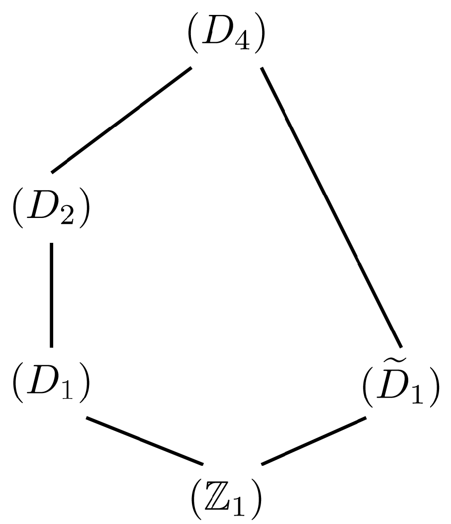
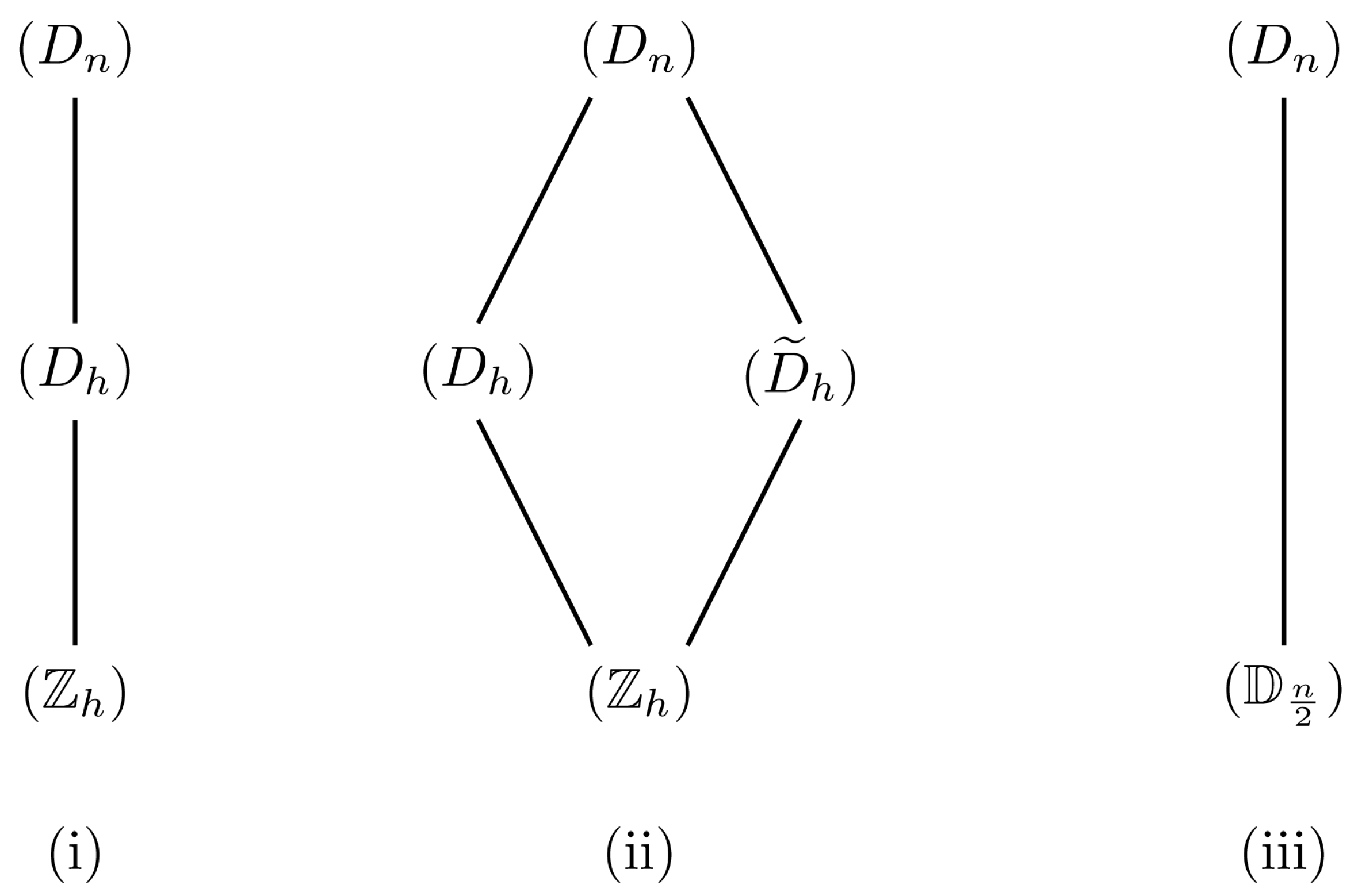
Appendix 2: Dihedral Group and Its Representations
A2.1. Dihedral Group
Represent the dihedral group, , of order as the group of rotations, one, γ, , ..., , of the complex plane (where is the multiplication by ) plus the reflections, κ, , , ..., , with κ being the operator of complex conjugation described by the matrix, .
To describe (up to conjugacy) subgroups of , take a positive integer, k, with , and . The list of subgroups of includes:
(i) the subgroups and their isomorphic copies:
, which are all conjugate, if is odd, but split into two conjugacy classes, and , where , if is even;
(ii) the cyclic subgroups, , generated by ξ.
A2.2. Irreducible -Representations and Basic Degrees
For the complete list of irreducible -representations and the corresponding basic degrees, we refer the reader, for instance, to [25], p. 174. Here, we restrict ourselves with the data important for the present paper.
(a) Clearly, there is the one-dimensional trivial representation, . In this case:
(b) For every integer number, , there is a -representation, , on given by:
where denotes the usual complex multiplication. Put:
For the lattices of orbit types related to this case, we refer to Figure 2i (the case, q, is odd) and Figure 2ii (the case, q, is even). Furthermore, we have the following degrees of the basic maps:
(c) For n being even, there is an irreducible representation, , given by , such that . In this case, the lattice of orbit types is given in Figure 2iii and the degree of the corresponding basic map is:
Figure 2.
Lattices of orbit types for irreducible -representations.
A2.3. -Representations Induced by Coordinate Permutations
Assume that is the natural -representation with the -action defined on the generators as follows:
where . Clearly, the matrices of transformation (72) and (73) are:
and:
respectively.
Proposition 5.6. Let V be a -representation given by (72) and (73) (see also (74) and (75)), and let . Then:
(i) V admits the isotypical decomposition:
where , (see Appendix 1);
(ii) for any collection of real numbers, , here exists a unique -equivariant linear operator, , such that .
(iii) Let C be a matrix of the operator, , provided by (ii). Then:
(a) if n is odd, then:
(b) if n is even, then:
References
- Coddington, E.; Levenson, N. Theory of Ordinary Differential Equations; McGraw-Hill: New York, NY, USA, 1955. [Google Scholar]
- Hartman, P. Ordinary Differential Equations; John Wiley & Sons: New York, NY, USA, 1964. [Google Scholar]
- Mawhin, J. Seventy-Five Years of Global Analysis around the Forced Pendulum Equation. In Proceedings of the Equadiff 9 Proceedings, Conference on Differential Equations and Their Applications, Brno, Czech Republic, 25–29 August 1997; Agarwal, R.P., Neuman, F., Vosmanský, J., Eds.; Masaryk University: Brno, Czech Republic, 1998; pp. 115–145. [Google Scholar]
- Hartman, P. On boundary value problems for systems of ordinary nonlinear second order differential equations. Trans. Am. Math. Soc. 1960, 96, 493–509. [Google Scholar] [CrossRef]
- Knobloch, H.W. On the existence of periodic solutions for second order vector differential equations. J. Differ. Eq. 1971, 9, 67–85. [Google Scholar] [CrossRef]
- Bebernes, J.W.; Schmidt, K. Periodic boundary value problems for systems of second order differential equations. J. Differ. Eq. 1973, 13, 33–47. [Google Scholar] [CrossRef]
- Mawhin, J. Some boundary value problems for Hartman-type perturbations of the ordinary vector p-Laplacian. Nonlinear Anal. TMA 2000, 40, 497–503. [Google Scholar] [CrossRef]
- Mawhin, J. Periodic Solutions of Systems with p-Laplacian-Like Operator. In Nonlinear Analysis and its Applications to Differential Equations; Progress in Nonlinear Differential Equations and Their Applications; Birkhäuser Boston: Boston, MA, USA, 2001; Volume 43, pp. 37–63. [Google Scholar]
- Mawhin, J.; Urena, A. A Hartman-Nagumo inequality for the vector ordinary p-Laplacian and applications to nonlinear boundary value problems. J. Inequal. Appl. 2002, 7, 701–725. [Google Scholar] [CrossRef]
- Balanov, Z.; Krawcewicz, W.; Nguyen, M. Multiple Solutions to Implicit Symmetric Boundary Value Problems for Second Order ODEs: Equivariant Degree Approach. Nonlinear Anal. Theory Methods Appl. 2013, 94, 45–64. [Google Scholar] [CrossRef]
- Balanov, Z.; Krawcewicz, W.; Rybicki, S.; Steinlein, H. A short treatise on the equivariant degree theory and its applications. J. Fixed Point Theory Appl. 2010, 8, 1–74. [Google Scholar] [CrossRef]
- Dzedzej, Z. Equivariant degree of convex-valued maps applied to set-valued BVP. Cent. Eur. J. Math. 2012, 10, 2173–2186. [Google Scholar] [CrossRef]
- Petryshyn, W.V. Solvability of various boundary value problems for the equation x′′ = f(t, x, x′, x′′) - y. Pac. J. Math. 1986, 122, 169–195. [Google Scholar] [CrossRef]
- Erbe, L.; Krawcewicz, W. Nonlinear boundary value problems for differential inclusions y′′ ∈ F(t, y, y′). Ann. Pol. Math. 1991, 3, 195–226. [Google Scholar]
- Erbe, L.; Krawcewicz, W.; Kaczynski, T. Solvability of two-point boundary value problems for system of nonlinear differential equations of the form y′′ = g(t, y, y′, y′′). Rocky Mount. J. Math. 1990, 20, 899–907. [Google Scholar] [CrossRef]
- Golubitsky, M.; Stewart, I.N.; Schaeffer, D.G. Singularities and Groups in Bifurcation Theory; Applied Mathematical Sciences 69; Springer: New York, NY, USA, 1988; Volume II. [Google Scholar]
- Balanov, Z.; Schwartzman, E. Morse complex, even functionals and asymptotically linear differential equations with resonance at infinity. Topol. Methods Nonlinear Anal. 1998, 12, 323–366. [Google Scholar]
- Bartsch, T. Topological Methods for Variational Problems with Symmetries. In Lecture Notes in Mathematics 1560; Springer: Berlin, Germany, 1993. [Google Scholar]
- Mawhin, J.; Willem, M. Critical Point Theory and Hamiltonian Systems; Applied Mathematical Sciences 74; Springer: New York, NY, USA, 1989. [Google Scholar]
- Rabinowitz, P.H. Minimax Methods in Critical Point Theory with Applications to Differential Equations; American Mathematical Society: Providence, RI, USA, 1986. [Google Scholar]
- Dihedral Calculator Home Page. Available online: http://dihedral.muchlearning.org/ (accessed on 31 October 2013).
- Ize, J.; Vignoli, A. Equivariant Degree Theory. In De Gruyter Series in Nonlinear Analysis and Applications; Walter de Gruyter: Berlin, Germany, 2003; Volume 8. [Google Scholar]
- Krawcewicz, W.; Wu, J. Theory of Degrees with Applications to Bifurcations and Differential Equations. In Canadian Mathematical Society Series of Monographs and Advanced Texts; John Wiley & Sons: New York, NY, USA, 1997. [Google Scholar]
- Kushkuley, A.; Balanov, Z. Geometric Methods in Degree Theory for Equivariant Maps. In Lecture Notes in Mathematics 1632; Springer-Verlag: Berlin, Germany, 1996. [Google Scholar]
- Balanov, Z.; Krawcewicz, W.; Steinlein, H. Applied Equivariant Degree. In AIMS Series on Differential Equations & Dynamical Systems; AIMS: Springfield, IL, USA, 2006; Volume 1. [Google Scholar]
- Dieck, T. Transformation Groups; Walter de Gruyter: Berlin, Germany, 1987. [Google Scholar]
- Borisovich, G.; Gelman, B.D.; Myshkis, A.D.; Obukhovskii, V.V. Introduction to the Theory of Multivalued Mappings and Differential Inclusions; URSS: Moscow, Russian, 2005. [Google Scholar]
- Bredon, G.E. Introduction to Compact Transformation Groups; Academic Press: New York, NY, USA, 1972. [Google Scholar]
- Kawakubo, K. The Theory of Transformation Groups; The Clarendon Press: Oxford, UK, 1991. [Google Scholar]
- Bröcker, T.; Dieck, T. Representations of Compact Lie Groups; Springer-Verlag: Berlin, Germany, 1985. [Google Scholar]
- Gorniewicz, L. Topological Fixed Point Theory of Multivalued Mappings; Springer: Berlin, Germany, 1999; Volume 495. [Google Scholar]
- Pruszko, T. Some applications of the topological degree theory to multivalued boundary value problems. Diss. Math. 1984, 229, 1–48. [Google Scholar]
- Pruszko, T. Topological degree methods in multivalued boundary value problems. Nonlinear Anal. 1978, 2, 263–309. [Google Scholar]
- Davis, P.J. Circulant Matrices; John Wiley and Sons: New York, NY, USA, 1979. [Google Scholar]
© 2013 by the authors; licensee MDPI, Basel, Switzerland. This article is an open access article distributed under the terms and conditions of the Creative Commons Attribution license (http://creativecommons.org/licenses/by/3.0/).